Inference and testing for structural change in time series of counts model

Paul DOUKHAN^∗ and William KENGNE

AGM, Université de Cergy Pontoise, 2 avenue Adolphe Chauvin. 95302 Cergy-Pontoise, France ().
^∗ IUF, Universitary institute of France.
E-mail: paul.doukhan@u-cergy.fr ; william.kengne@u-cergy.fr

Abstract : We consider here together the inference questions and the change-point problem in Poisson autoregressions (see Tjøstheim, 2012). The conditional mean (or intensity) of the process is involved as a non-linear function of it past values and the past observations. Under Lipschitz-type conditions, it is shown that the conditional mean can be written as a function of lagged observations. In the latter model, assume that the link function depends on an unknown parameter $\theta_{0}$. The consistency and the asymptotic normality of the maximum likelihood estimator of the parameter are proved. These results are used to study change-point problem in the parameter $\theta_{0}$. We propose two tests based on the likelihood of the observations. Under the null hypothesis (i.e. no change), it is proved that both those test statistics converge to an explicit distribution. Consistencies under alternatives are proved for both tests. Simulation results show how those procedure work practically, and an application to real data is also processed.  
 

Keywords: time series of counts; Poisson autoregression; likelihood estimation; change-point; semi-parametric test.

1 Introduction

Count models are of a large current interest, see the discussion paper Tjøstheim (2012). Integer-valued time series appear as natural for modeling count events. Examples may be found in epidemiology (number of new infections), in finance (number of transactions per minute), in industrial quality control (number of defects); see for instance Held et al. (2005), Brännäs and Quoreshi (2010) and Lambert (1992).
Real data are definitely not stationary. Several ways to consider such structural changes are possible as this was demonstrated during the thematic cycle Nonstationarity and Risk Management held in Cergy-Pontoise during year 2012 (). Structural breaks are a reasonable possibility for this, when no additional knowledge is available. The paper is thus aimed at considering such changes in regime for a large class of integer valued time series.
Let $Y=(Y_{t})_{t\in{\bf Z}}$ be an integer-valued time series and $\mathcal{F}_{t}=\sigma(Y_{s},~{}s\leq t)$ the $\sigma$-field generated by the whole past at time $t$, we denote by $\mathcal{L}(Y_{t}/\mathcal{F}_{t-1})$ the conditional distribution of $Y_{t}$ given the past. Models with various marginal distributions and dependence structures have been studied for instance Kedem and Fokianos (2002), Davis et al. (2005), Ferland et al. (2006), Davis and Wu (2009), Wei$\ss$ (2009).
Fokianos et al. (2009) considered the Poisson autoregression such that $\mathcal{L}(Y_{t}/\mathcal{F}_{t-1})$ is Poisson distributed with a intensity $\lambda_{t}$ which is a function of $\lambda_{t-1}$ and $Y_{t-1}$. Under linear autoregression, they prove both the consistency and the asymptotic normality of the maximum likelihood estimator of the regression parameter, by using a perturbation approach, which allows to used the standard Markov ergodic setting. Fokianos and Tjøstheim (2012) extend the method to nonlinear Poisson autoregression with $\lambda_{t}=f(\lambda_{t-1})+b(Y_{t-1})$ for nonlinear measurable functions $f$ and $b$. In the same vein, Neumann (2011) had studied some large situation where $\lambda_{t}=f(\lambda_{t-1},Y_{t-1})$. He focused on the absolute regularity and the specification test for the intensity function, while the recent work of Fokianos and Neumann (2013) studied goodness-of-fit tests which are able to detect local alternatives. Doukhan et al. (2012), consider a more general model with infinitely many lags. Stationarity and the existence of moments are proved by using a weak dependent approach and contraction properties.
Later, Davis and Liu (2012) studied the model where the distribution $\mathcal{L}(Y_{t}/\mathcal{F}_{t-1})$ belongs to a class of one-parameter exponential family with finite order dependence. This class contains Poisson and negative binomial distribution. From the theory of iterated random functions, they establish the stationarity and the absolute regularity properties of the process. They also prove the consistency and asymptotic normality of the maximum likelihood estimator of the parameter of the model.
Douc et al. (2012) considers a class of observation-driven time series which covers linear, log-linear, and threshold Poisson autoregressions. They approach is based on a recent theory for Markov chains based upon Hairer and Mattingly (2006) recent work; this allows existence and uniqueness of the invariant distribution for Markov chains without irreducibility. They also proved consistency of the conditional likelihood estimator of the model (even under false models); the asymptotic normality is not yet considered in this setting.
For change point procedures, Kang and Lee (2009) proposed CUSUM procedure for testing for parameter change in a first-order random coefficient integer-valued autoregressive model defined through thinning operator. Fokianos and Fried (2010, 2012) studied mean shift in linear and log-linear Poisson autoregression. The dependence between the level shift and time allows their model to detect several types of interventions effects such as outliers. Franke et al. (2012) consider parameter change in Poisson autoregression of order one. Their test are based on the cumulative sum of residuals using conditional least-squares estimator.

In this article, we first consider a time series of counts $Y=(Y_{t})_{t\in{\bf Z}}$ satisfying :

$$Y_{t}/\mathcal{F}_{t-1}\sim\mbox{ Poisson}(\lambda_{t})~{}\text{with}~{}\lambda_{t}=F(\lambda_{t-1},\ldots;Y_{t-1},\ldots)$$ (1)

where $\mathcal{F}_{t}=\sigma(Y_{s},~{}s\leq t)$ and $F$ a measurable non-negative function. The properties of the general class of Poisson autoregression model (1) have been studied by Doukhan et al. [13]. According to the fact that the model (1) can take into account the whole past information of the process, it dependence structure is more general than those studied before. Proceeding as in Doukhan and Wintenberger (2008), we show that under some Lipschitz-type conditions on $F$, the conditional mean $\lambda_{t}$ can be written as a function of the past observations. This leads us to consider the model

$$Y_{t}/\mathcal{F}_{t-1}\sim\mbox{ Poisson}(\lambda_{t})~{}\text{with}~{}\lambda_{t}=f(Y_{t-1},\ldots)$$ (2)

where $f$ is a measurable non-negative function. We assume that $f$ is know up to some parameter $\theta_{0}$ belonging to a compact set $\Theta$. That is

$$Y_{t}/\mathcal{F}_{t-1}\sim\mbox{ Poisson}(\lambda_{t})~{}\text{with}~{}\lambda_{t}=f_{\theta_{0}}(Y_{t-1},\ldots)~{}\,\,\,\text{and}\,\,\,~{}\theta_{0}\in\Theta.$$ (3)

Many classical integer-valued time series satisfying (3) (see the examples below).
Remark that, model (3) (as well as models (1) and (2)) can be represented in terms of Poisson processes. Let $(N_{t})_{t\geq 0}$ be a sequence of independent Poisson processes of unit intensity. $Y_{t}$ can be seen as a number (say $N_{t}(\lambda_{t})$) of events that occurred in the time interval $[0,\lambda_{t}]$. So, we have the representation

$$Y_{t}=N_{t}(\lambda_{t})~{}\text{with}~{}\lambda_{t}=f_{\theta_{0}}(Y_{t-1},\ldots).$$ (4)

The paper is first work out the asymptotic properties of the maximum likelihood estimator of the model (3). We assume that the function $f_{\theta}$ satisfies some classical Lipschitz-type inequality and investigate sufficient conditions for the consistency and the asymptotic normality of the maximum likelihood estimator of $\theta_{0}$. Contrary to Fokianos et al. [19] the increasing of the function $(y_{k})_{k\in I\!\!N}\mapsto f_{\theta}((y_{k})_{k\in I\!\!N})$ (not easy to define here) as well as the existence of the fourth order derivative of the function $\theta\mapsto f_{\theta}$ are not needed. Although the models studied by Davis and Liu [9] and Douc et al. [11] allow large classes of marginal distributions, the infinitely many lags of model (1) (or model (3)) makes it allows a large type of dependence structure.

The second contribution of this work are the two tests for change detection in model (3). We propose a new idea to take into account the change-point alternative. This make that, the procedures proposed will be numerically easy to apply than that proposed by Kengne (2012). The consistency under the alternative are proved. Contrary to Franke et al. [20], the multiple change alternative has been considered and the independence between the observation before and after the change-point is not assumed. Note that, the intervention problem studied by Fokianos and Fried [15, 16] is intended to sudden shift in the conditional means of the process. In the classical change-point setting, such intervention will be asymptotically negligible.

In the forthcoming Section 2, it is provided some assumptions on model with examples. Section 3 is devoted to the definition of the maximum likelihood estimator with it asymptotic properties. In Section 4, we propose the tests for detecting change in parameter of model (3). Some simulation results and real data application are presented in Sections 5 and 6 and the proofs of the main results are provided in Section 7.

2 Assumptions and examples

2.1 Assumptions

We will use the following classical notations:

1. $\|y\|:=\sum\limits_{j=1}^{p}|y_{j}|$ for any $y\in I\!\!R^{p}$;

2. for any compact set $\mathcal{K}\subseteq I\!\!R^{d}$ and for any function $g:\mathcal{K}\longrightarrow I\!\!R^{d^{\prime}}$, $\|g\|_{\mathcal{K}}=\sup_{\theta\in\mathcal{K}}(\|g(\theta)\|)$;

3. it $Y$ is a random variable with finite moment of order $r>0$, then $\|Y\|_{r}=(E\,|Y|^{r})^{1/r}$;

4. for any set $\mathcal{K}\subseteq I\!\!R^{d}$, $\overset{\circ}{\mathcal{K}}$ denotes the interior of $\mathcal{K}$.

A classical Lipschitz-type conditions is assumed on the model (1).

Assumption A_F : There exists a sequence of non-negative real numbers $(\alpha_{j})_{j\geq 1}$ satisfying $\sum\limits_{j=1}^{\infty}\alpha_{j}<1$ and such that for any $y,y^{\prime}\in((0,\infty)\times I\!\!N)^{I\!\!N}$,

$$|F(y)-F(y^{\prime})|\leq\sum\limits_{j=1}^{\infty}\alpha_{j}\|y_{j}-y^{\prime}_{j}\|.$$

Under assumption (A_F), Doukhan et al. [13] have shown that there exists a solution $(Y_{t},\lambda_{t})_{t\in{\bf Z}}$ which is $\tau$-weakly dependent strictly stationary with finite moment of any order. The following proposition show that the conditional mean $\lambda_{t}$ of model (1) can be expressed as a function of only the past observations of the process.

Proposition 2.1

Under (A_F), there exists a measurable function $f:I\!\!R^{+}\rightarrow I\!\!R^{+}$ such that the strictly stationary ergodic solution of model (1) satisfying almost surely

$$\lambda_{t}=f(Y_{t-1},\dots).$$

Proposition 2.1 shows that, the information contained in the unobservable process $(\lambda_{t-j})$ can be capture by the observable process $(Y_{t-j})$. This shows that, in practice the autoregression on $(Y_{t-j})$ is sufficient to capture the information of the whole past. This representation is very important in the inference framework. Note that, if one carries inference on the model (1) by assuming that $\lambda_{t}=F_{\theta_{0}}(\lambda_{t-1},\ldots;Y_{t-1},\ldots)$, it will not be easy to compute $\partial\lambda_{t}/\partial\theta$ or to write it as a function of $\partial F_{\theta}/\partial\theta$. So, the asymptotic normality of the maximum likelihood estimator of $\theta_{0}$ (see (7) and (8)) will be very difficult to study.
We focus on the model (3) with the following assumptions. For $i=0,\,1,\,2$ and for any compact set $\mathcal{K}\subseteq\Theta$, define
Assumption A${}_{i}(\mathcal{K})$: $\|{\partial^{i}f_{\theta}(0)}/{\partial\theta^{i}}\|_{\Theta}<\infty$ and there exists a sequence of non-negative real numbers $(\alpha^{(i)}_{k}(\mathcal{K}))_{k\geq 1}$ satisfying $\sum\limits_{j=1}^{\infty}\alpha^{(0)}_{k}(\mathcal{K})<1$ or $\sum\limits_{j=1}^{\infty}\alpha^{(i)}_{k}(\mathcal{K})<\infty$ (for $i=1,2$) such that

$$\Big{\|}\dfrac{\partial^{i}f_{\theta}(y)}{\partial\theta^{i}}-\dfrac{\partial^{i}f_{\theta}(y^{\prime})}{\partial\theta^{i}}\Big{\|}_{\mathcal{K}}\leq\sum\limits_{k=1}^{\infty}\alpha^{(i)}_{k}(\mathcal{K})|y_{k}-y^{\prime}_{k}|\quad\mbox{ for all }y,y^{\prime}\in(I\!\!R^{+})^{I\!\!N}.$$

The Lipschitz-type condition A${}_{0}(\Theta)$ is the version of model (3) of the assumption A_F. It is classical when studying the existence of solutions of such model (see for instance [12], [1] or [13]). The assumptions A${}_{1}(\mathcal{K})$ and A${}_{2}(\mathcal{K})$ as well as the following assumptions D$(\Theta)$, Id($\Theta$) and Var($\Theta$) are needed to define and to study the asymptotic properties of the maximum likelihood estimator of the model (3).

Assumption D$(\Theta)$: $\exists\underline{c}>0$ such that $\displaystyle\inf_{\theta\in\Theta}(f_{\theta}(y))\geq\underline{c}$ for all $y\in(I\!\!R^{+})^{I\!\!N}.$
 
Assumption Id($\Theta$): For all $(\theta,\theta^{\prime})\in\Theta^{2}$, $\Big{(}f_{\theta}(Y_{t-1},\dots)=f_{\theta^{\prime}}(Y_{t-1},\dots)\ \text{a.s.}~{}\text{ for some }t\in{\bf Z}\Big{)}\Rightarrow\ \theta=\theta^{\prime}.$ Assumption Var($\Theta$): For all $\theta\in\Theta$ and $t\in{\bf Z}$, the components of the vector $\dfrac{\partial f_{\theta}}{\partial\theta^{i}}(Y_{t-1,\dots})$ are a.s. linearly independent.

2.2 Examples

2.2.1 Linear Poisson autoregression

We consider an integer-valued time series $(Y_{t})_{t\in{\bf Z}}$ satisfying for any $t\in{\bf Z}$

$$Y_{t}/\mathcal{F}_{t-1}\sim\mbox{ Poisson}(\lambda_{t})~{}\text{with}~{}\lambda_{t}=\phi_{0}(\theta_{0})+\sum_{k\geq 1}\phi_{k}(\theta_{0})Y_{t-k}$$ (5)

where $\theta_{0}\in\Theta\subset I\!\!R^{d}$, the function $\theta\mapsto\phi_{k}(\theta)$ are positive and satisfying $\sum_{k\geq 1}\left\|\phi_{k}(\theta)\right\|_{\Theta}<1$. Assumptions A${}_{0}(\Theta)$ holds automatically. If the function $\phi_{k}$ are twice continuous differentiable such that $\sum_{k\geq 1}\left\|\phi_{k}^{\prime}(\theta)\right\|_{\Theta}<\infty$ and $\sum_{k\geq 1}\left\|\phi_{k}^{\prime\prime}(\theta)\right\|_{\Theta}<\infty$ then A${}_{1}(\Theta)$ and A${}_{2}(\Theta)$ hold. If $\underset{\theta\in\Theta}{\inf}\phi_{0}(\theta)>0$ then D$(\Theta)$ holds. Moreover, if there exists a finite subset $I\subset I\!\!N-\{0\}$ such that the function $\theta\mapsto(\phi_{k}(\theta))_{k\in I}$ is injective, then assumption Id$(\Theta)$ holds i.e. model (5) is identifiable.
Note that the popular Poisson INGARCH model (see [14] or [32]) is a special case of model (5). Finally, the model (5) can be generalized by considering

$$\lambda_{t}=\phi_{0}(\theta_{0})+\sum_{k\geq 1}\phi_{k}(\theta_{0})h(Y_{t-k})$$

where $h$ is a Lipschitz function. The threshold model can be obtained with $h(y)=(y-\ell)_{+}$ for some $\ell>0$, where $y_{+}=\max(y,0)$.

2.2.2 Power Poisson autoregression

We consider a power Poisson INGARCH($p,q$) process defined by

$$Y_{t}/\mathcal{F}_{t-1}\sim\mbox{ Poisson}(\lambda_{t})~{}\text{with}~{}\lambda_{t}=\Big{(}\alpha_{0}(\theta_{0})+\sum_{k=1}^{p}\alpha_{k}(\theta_{0})\lambda_{t-k}^{\delta}+\sum_{k=1}^{q}\beta_{k}(\theta_{0})Y_{t-k}^{\delta}\Big{)}^{1/\delta}$$ (6)

where $\delta\geq 1$, $\theta_{0}\in\Theta\subset I\!\!R^{d}$ and the function $\theta\mapsto\alpha_{k}(\theta)$ and $\theta\mapsto\beta_{k}(\theta)$ are positive. If $\sum_{k=1}^{p}\left\|\alpha_{k}(\theta)\right\|_{\Theta}^{1/\delta}+\sum_{k=1}^{q}\left\|\beta_{k}(\theta)\right\|_{\Theta}^{1/\delta}<1$, then the Lipschitz-type condition (A_F) is satisfied. In this case, we can find a sequence of non-negative function $(\psi_{k}(\theta))_{k\geq 1}$ such that $\lambda_{t}=\Big{(}\psi_{0}(\theta_{0})+\sum_{k\geq 1}\psi_{k}(\theta_{0})Y_{t-k}^{\delta}\Big{)}^{1/\delta}$. If $\underset{\theta\in\Theta}{\inf}\alpha_{0}(\theta)>0$ then D$(\Theta)$ holds. Moreover, if there exists a finite subset $I\in I\!\!N-\{0\}$ such that the function $\theta\mapsto(\psi_{k}(\theta))_{k\in I}$ is injective, then assumption Id$(\Theta)$ holds i.e. model (6) is identifiable.

3 Likelihood inference

Assume that the trajectory $(Y_{1},\dots,Y_{n})$ is observed. The conditional (log)-likelihood (up to a constant) of model $(3)$ computed on $T\subset\{1,\dots,n\}$, is given by

$$L_{n}(T,\theta)=\sum_{t\in T}(Y_{t}\log\lambda_{t}(\theta)-\lambda_{t}(\theta))=\sum_{t\in T}\ell_{t}(\theta)\,\,\,\text{with}\,\,\,\ell_{t}(\theta)=Y_{t}\log\lambda_{t}(\theta)-\lambda_{t}(\theta)$$

where $\lambda_{t}(\theta)=f_{\theta}(Y_{t-1},\dots)$. In the sequel, we use the notation $f^{t}_{\theta}:=f_{\theta}(Y_{t-1},\ldots).$ Since only $Y_{1},\dots,Y_{n}$ are observed, we will use an approximation version of the (log)-likelihood defined by

$$\widehat{L}_{n}(T,\theta)=\sum_{t\in T}(Y_{t}\log\widehat{\lambda}_{t}(\theta)-\widehat{\lambda}_{t}(\theta))=\sum_{t\in T}\widehat{\ell}_{t}(\theta)\,\,\,\text{with}\,\,\,\widehat{\ell}_{t}(\theta)=Y_{t}\log\widehat{\lambda}_{t}(\theta)-\widehat{\lambda}_{t}(\theta)$$ (7)

where $\widehat{\lambda}_{t}(\theta):=\widehat{f}^{t}_{\theta}:=f_{\theta}(Y_{t-1},\dots,Y_{1},0,\dots)$ and $\widehat{\lambda}_{1}(\theta)=f_{\theta}(0,\dots)$. The maximum likelihood estimator (MLE) of $\theta_{0}$ computed on $T$ is defined by

$$\widehat{\theta}_{n}(T)=\operatorname{argmax}_{\theta\in\Theta}(\widehat{L}_{n}(T,\theta)).$$ (8)

For any $k,k^{\prime}\in{\bf Z}$ such as $k\leq k^{\prime}$, denote

$$T_{k,k^{\prime}}=\{k,k+1,\ldots,k^{\prime}\}.$$

Theorem 3.1

Let $(j_{n})_{n\geq 1}$ and $(k_{n})_{n\geq 1}$ be two integer valued sequences such that $j_{n}\leq k_{n}$, $k_{n}\to+\infty$ and $k_{n}-j_{n}\to+\infty$ as $n\to+\infty$. Assume $\theta_{0}\in\ring{\Theta}$ and $D(\Theta)$, $\mathrm{Id}(\Theta)$ and $A_{0}(\Theta)$ hold with

$$\sum_{j\geq 1}\log j\times\alpha_{j}^{(0)}(\Theta)<\infty.$$ (9)

It holds that

$$\widehat{\theta}_{n}(T_{j_{n},k_{n}})\xrightarrow[n\to+\infty]{a.s.}\theta_{0}.$$

The following theorem shows the asymptotic normality of the MLE of model (3).

Theorem 3.2

Let $(j_{n})_{n\geq 1}$ and $(k_{n})_{n\geq 1}$ be two integer valued sequences such that $j_{n}\leq k_{n}$, $k_{n}\to+\infty$ and $k_{n}-j_{n}\to+\infty$ as $n\to+\infty$. Assume $\theta_{0}\in\ring{\Theta}$ and $D(\Theta)$, $\mathrm{Id}(\Theta)$, Var($\Theta$) and $A_{i}(\Theta)$ $i=0,1,2$ hold with

$$\sum_{j\geq 1}\sqrt{j}\times\alpha_{j}^{(i)}(\Theta)<\infty.$$ (10)

It holds that

$$\sqrt{k_{n}-j_{n}}(\widehat{\theta}_{n}(T_{j_{n},k_{n}})-\theta_{0})\xrightarrow[n\to+\infty]{\mathcal{D}}\mathcal{N}(0,\Sigma^{-1})$$

where $\Sigma=E\big{(}\frac{1}{f_{\theta_{0}}^{0}}(\frac{\partial}{\partial\theta}f^{0}_{\theta_{0}})(\frac{\partial}{\partial\theta}f^{0}_{\theta_{0}})^{\prime}\big{)}.$

According to the Lemma 7.1 and the proof of Theorem 3.2, the matrix

$$\Big{(}\frac{1}{k_{n}-j_{n}}\sum_{t=j_{n}}^{k_{n}}\frac{1}{\widehat{f}_{\theta}^{t}}\big{(}\frac{\partial}{\partial\theta}\widehat{f}_{\theta}^{t}\big{)}\big{(}\frac{\partial}{\partial\theta}\widehat{f}_{\theta}^{t}\big{)}^{\prime}\Big{)}\Big{|}_{\theta=\widehat{\theta}_{n}(T_{j_{n},k_{n}})}\,\,\,\text{and}\,\,\,\Big{(}-\dfrac{1}{k_{n}-j_{n}}\dfrac{\partial^{2}}{\partial\theta\partial\theta^{\prime}}\widehat{L}_{n}(T_{j_{n},k_{n}},\theta)\Big{)}\Big{|}_{\theta=\widehat{\theta}_{n}(T_{j_{n},k_{n}})}$$

are consistent estimators of the covariance matrix $\Sigma$.

Remark 3.1

1. In Theorems 3.1 and 3.2, the typical sequences $j_{n}=1$ and $k_{n}=n$, $\forall n\geq 1$ can be chosen. This choice is the case where the estimator is computed with all the observations. But in the change-point study, the estimator needs to be calculated over a part of the observations. Results are written this way to cover the change point situation.

2. If the Lipschitz coefficients $(\alpha_{j}^{(i)}(\Theta))_{j\geq 1}$ satisfy $\alpha_{j}^{(i)}(\Theta)=\mathcal{O}(j^{-\gamma})$ with $\gamma>1/2$, then the conditions (9) and (10) of Theorem 3.1 and Theorem 3.2 hold.

4 Testing for Parameter Changes

We consider the observations $Y_{1},\dots,Y_{n}$ generated as in model $(3)$ and assume that the parameter $\theta_{0}$ may change over time. More precisely, we assume that $\exists K\geq 1,\theta_{1}^{*},\dots,\theta_{K}^{*}\in\Theta,0=t_{0}^{*}<t_{1}^{*}<\dots<t_{K-1}^{*}<t_{K}^{*}=n$ such that $Y_{t}=Y_{t}^{(j)}$ for $t^{*}_{j-1}<t\leq t^{*}_{j}$, where the process $(Y_{j}^{(j)})_{t\in{\bf Z}}$ is a stationary solution of $(3)$ depending on $\theta^{*}_{j}$. The case where the parameter does not change corresponds to $K=1$. For this problem, we consider the following hypothesis:

1. The observations $(Y_{1},\dots,Y_{n})$ are a trajectory of a process $(Y_{t})_{t\in{\bf Z}}$ solution of $(3)$, depending on $\theta_{0}\in\Theta$.

2. There exists $K\geq 2,\theta_{1}^{*},\theta_{2}^{*},\dots,\theta_{K}^{*}$ with $\theta_{1}^{*}\neq\theta_{2}^{*}\neq\dots\neq\theta_{K}^{*},0=t_{0}^{*}<t_{1}^{*}<\cdots<t_{K-1}^{*}<t_{K}^{*}=n$ such that the observations $(Y_{t})_{t^{*}_{j-1}<t\leq t^{*}_{j}}$ are a trajectory of the process $(Y_{t}^{(j)})_{t\in{\bf Z}}$ solution of $(3)$, depending on $\theta^{*}_{j}$.

Let us note that, contrary to Franke et al. (2012), the independence between the observations before and after the change-point is not assumed. Moreover, we can consider more complex parameter in the model, not only the constant term of the conditional mean as in [20]. In the case of linear Poisson autoregression, the assumption (A9) of their model leads to the change in the unconditional mean. Therefore, our change-point problem is more general.

Remark 4.1

Let $\lambda^{(j)}_{t}$ be the conditional mean on the segment $T^{*}_{j}=\{t^{*}_{j-1},t^{*}_{j-1}+1,\ldots,t^{*}_{j}\}$. By using the representation (4), we can write

$$Y_{t}^{(j)}=N_{t}(\lambda_{t}^{(j)})\,\,\,\text{with}\,\,\,\lambda^{(j)}_{t}=f_{\theta^{*}_{j}}(Y_{t-1}^{(j)},\ldots).$$

We can also write

$$Y_{t}^{(j)}=\tilde{F}(Y_{t-1}^{(j)},\ldots;N_{t})\,\,\,\text{where}\,\,\,\tilde{F}(y_{1},y_{2},\ldots;N_{t})=N_{t}(f_{\theta^{*}_{j}}(y_{1},y_{2},\ldots))\,\,\,\text{for any}\,\,\,y_{k}\in I\!\!N,~{}k\geq 1.$$

So, for any $y=(y_{k})_{k\geq 1}$ and $y^{\prime}=(y^{\prime}_{k})_{k\geq 1}$, we have

$$E\,|\tilde{F}(y;N_{t})-\tilde{F}(y^{\prime};N_{t})|=E\,|N_{t}(f_{\theta^{*}_{j}}(y))-N_{t}(f_{\theta^{*}_{j}}(y^{\prime}))|=|f_{\theta^{*}_{j}}(y)-f_{\theta^{*}_{j}}(y^{\prime})|\leq\sum_{k\geq 1}\alpha^{(0)}_{k}|y_{k}-y^{\prime}_{k}|,$$ (11)

where the second equality follows by seen $|N_{t}(f_{\theta^{*}_{j}}(y))-N_{t}(f_{\theta^{*}_{j}}(y^{\prime}))|$ as a number of events $N_{t}$ that occur in the time interval $[0,|f_{\theta^{*}_{j}}(y)-f_{\theta^{*}_{j}}(y^{\prime})|]$.
Let $(\widetilde{Y}_{t},\widetilde{\lambda}_{t})_{t^{*}_{j-1}<t\leq t^{*}_{j}}$ be the nonstationary approximation of the process $(Y_{t}^{(j)},\lambda_{t}^{(j)})_{t\in{\bf Z}}$ on the segment $T^{*}_{j}$; i.e.

$$\widetilde{Y}_{t}=N_{t}(\widetilde{\lambda}_{t})\,\,\,\text{with}\,\,\,\widetilde{\lambda}_{t}=f_{\theta^{*}_{j}}(Y_{t-1}^{(j)},\ldots,Y_{t-t^{*}_{j-1}}^{(j)},Y_{t-t^{*}_{j-1}-1}^{(j-1)},\ldots,Y^{(1)}_{1},0,\ldots).$$

By using assumption A${}_{0}(\Theta)$ and relation (11), one can show that the approximated process $(\widetilde{Y}_{t},\widetilde{\lambda}_{t})_{t^{*}_{j-1}<t\leq t^{*}_{j}}$ converges (in $L^{r}$ for any $r\geq 1$) to the stationary regime (see for instance Bardet et al. [2] where similar apprimation has been done in the case of causal time series). So, the results of the Section 4.2 may be extended (modulo the validity of the approximation) by relaxing the stationarity assumption after change.

Recall that under H₀, the likelihood function of the model computed on $T\subset\{1,\dots,n\}$ is given by

$$\widehat{L}_{n}(T,\theta)=\sum_{t\in T}(Y_{t}\log\widehat{f}_{\theta}^{t}-\widehat{f}_{\theta}^{t})$$

where $\widehat{f}_{\theta}^{t}=f_{\theta}(Y_{t,1},\dots)$ and the maximum likelihood estimator is given by $\widehat{\theta}_{n}(T)=\operatorname{argmax}\widehat{L}_{n}(T,\theta)$. It holds from Theorem 3.2 that, under H₀, the asymptotic covariance matrix of $\widehat{\theta}_{n}(T_{1,n})$ is $\widehat{\Sigma}_{n}^{-1}$ where

$$\widehat{\Sigma}_{n}=\Big{(}\frac{1}{n}\sum_{t=1}^{n}\frac{1}{\widehat{f}_{\theta}^{t}}\big{(}\frac{\partial}{\partial\theta}\widehat{f}_{\theta}^{t}\big{)}\big{(}\frac{\partial}{\partial\theta}\widehat{f}_{\theta}^{t}\big{)}^{\prime}\Big{)}\Big{|}_{\theta=\widehat{\theta}_{n}(T_{1,n})}.$$

$\widehat{\Sigma}_{n}$ is a consistant estimator of

$$\Sigma=E\Big{(}\frac{1}{f^{0}_{\theta_{0}}}\big{(}\frac{\partial}{\partial\theta}f^{0}_{\theta_{0}}\big{)}\big{(}\frac{\partial}{\partial\theta}f^{0}_{\theta_{0}}\big{)}^{\prime}\Big{)}$$

under H₀ (see the proof of Theorem 3.2). The consistency of $\widehat{\Sigma}_{n}$ under H₁ is not ensured. $\widehat{\Sigma}_{n}$ does not take into account the change-point alternative. So, the consistency under H₁ of any test based on $\widehat{\Sigma}_{n}$ will not be easy to prove.

Let $(u_{n})_{n\geq 1}$ and $(u_{n})_{n\geq 1}$ be two integer valued sequences satisfying $u_{n},v_{n}\to+\infty,\frac{u_{n}}{n},\frac{v_{n}}{n}\to 0$ as $n\to+\infty$. Our test statistic is based on the following matrix

$$\widehat{\Sigma}_{n}(u_{n})=\frac{1}{2}\Big{[}\Big{(}\frac{1}{u_{n}}\sum_{t=1}^{u_{n}}\frac{1}{\widehat{f}_{\theta}^{t}}\big{(}\frac{\partial}{\partial\theta}\widehat{f}_{\theta}^{t}\big{)}\big{(}\frac{\partial}{\partial\theta}\widehat{f}_{\theta}^{t}\big{)}^{\prime}\Big{)}\Big{|}_{\theta=\widehat{\theta}_{n}(T_{1,u_{n}})}+\Big{(}\frac{1}{n-u_{n}}\sum_{t=u_{n}+1}^{n}\frac{1}{\widehat{f}_{\theta}^{t}}\big{(}\frac{\partial}{\partial\theta}\widehat{f}_{\theta}^{t}\big{)}\big{(}\frac{\partial}{\partial\theta}\widehat{f}_{\theta}^{t}\big{)}^{\prime}\Big{)}\Big{|}_{\theta=\widehat{\theta}_{n}(T_{u_{n}+1,n})}\Big{]}.$$

Theorem 3.1 and Lemma 7.1 show that $\widehat{\Sigma}_{n}(u_{n})$ is consistent under H₀. Under H₁, we will use the classical assumption that the breakpoint gown at rate $n$. This will allow us to show that the first component of $\widehat{\Sigma}_{n}(u_{n})$ converges to the covariance matrix of the stationary model of the first regime. It will be a key to prove the consistency under H₁.
Another way to deal is to consider the matrix

$$\widetilde{\Sigma}_{n}(u_{n})=\frac{1}{2}\Big{[}\Big{(}\frac{1}{n-u_{n}}\sum_{t=1}^{n-u_{n}}\frac{1}{\widehat{f}_{\theta}^{t}}\big{(}\frac{\partial}{\partial\theta}\widehat{f}_{\theta}^{t}\big{)}\big{(}\frac{\partial}{\partial\theta}\widehat{f}_{\theta}^{t}\big{)}^{\prime}\Big{)}\Big{|}_{\theta=\widehat{\theta}_{n}(T_{1,n-u_{n}})}+\Big{(}\frac{1}{u_{n}}\sum_{t=n-u_{n}+1}^{n}\frac{1}{\widehat{f}_{\theta}^{t}}\big{(}\frac{\partial}{\partial\theta}\widehat{f}_{\theta}^{t}\big{)}\big{(}\frac{\partial}{\partial\theta}\widehat{f}_{\theta}^{t}\big{)}^{\prime}\Big{)}\Big{|}_{\theta=\widehat{\theta}_{n}(T_{n-u_{n}+1,n})}\Big{]}.$$

Asymptotically, both the matrices $\widehat{\Sigma}_{n}(u_{n})$ and $\widetilde{\Sigma}_{n}(u_{n})$ have the same behavior under H₀. In the case of non stationarity after change, the procedure using $\widetilde{\Sigma}_{n}(u_{n})$ can provide more distortion; because due to the dependance the second component of $\widetilde{\Sigma}_{n}(u_{n})$ will converge very slowly than the first component of $\widehat{\Sigma}_{n}(u_{n})$.

Let us define now the tests statistics:

• $\displaystyle\widehat{C}_{n}=\max_{v_{n}\leq k\leq n-v_{n}}\widehat{C}_{n,k}$ where

  $$\widehat{C}_{n,k}=\frac{1}{q^{2}(\frac{k}{n})}\frac{k^{2}(n-k)^{2}}{n^{3}}\big{(}\widehat{\theta}_{n}(T_{1,k})-\widehat{\theta}_{n}(T_{k+1,n})\big{)}^{\prime}\widehat{\Sigma}_{n}(u_{n})\big{(}\widehat{\theta}_{n}(T_{1,k})-\widehat{\theta}_{n}(T_{k+1,n})\big{)};$$

  where $q$ is a weight function define on $(0,1)$, see bellow;

• $\displaystyle\widehat{Q}_{n}^{(1)}=\max_{v_{n}\leq k\leq n-v_{n}}\widehat{Q}_{n,k}^{(1)}$ where

  $$\widehat{Q}_{n,k}^{(1)}=\frac{k^{2}}{n}\big{(}\widehat{\theta}_{n}(T_{1,k})-\widehat{\theta}_{n}(T_{1,n})\big{)}^{\prime}\widehat{\Sigma}_{n}(u_{n})\big{(}\widehat{\theta}_{n}(T_{1,k})-\widehat{\theta}_{n}(T_{1,n})\big{)};$$

• $\displaystyle\widehat{Q}_{n}^{(2)}=\max_{v_{n}\leq k\leq n-v_{n}}\widehat{Q}_{n,k}^{(2)}$ where

  $$\widehat{Q}_{n,k}^{(2)}=\frac{(n-k)^{2}}{n}\big{(}\widehat{\theta}_{n}(T_{k+1,n})-\widehat{\theta}_{n}(T_{1,n})\big{)}^{\prime}\widehat{\Sigma}_{n}(u_{n})\big{(}\widehat{\theta}_{n}(T_{k+1,n})-\widehat{\theta}_{n}(T_{1,n})\big{)}.$$

The first procedure is based on the statistique $\widehat{C}_{n}$ and the other one is based on the statistic $\widehat{Q}_{n}$ defined by

$$\widehat{Q}_{n}:=\max(\widehat{Q}_{n}^{(1)},\widehat{Q}_{n}^{(2)}).$$

The weight function $q$ is used to increase the power of the test based on the statistic $\widehat{C}_{n}$. In the sequel, we will assume that
$q:(0,1)\rightarrow(0,\infty)$ is non-decreasing in a neighborhood of zero, non-increasing in a neighborhood of one and satisfying $\underset{\eta<\tau<1-\eta}{\inf}q(\tau)>0$ for all $0<\eta<1/2$.
The behavior of the weighted function $q$ can be controlled at the neighborhood of zero and one by the integral

$$I_{0,1}(q,c)=\int_{0}^{1}\dfrac{1}{t(1-t)}\exp\Big{(}-\dfrac{cq^{2}(t)}{t(1-t)}\Big{)}dt,~{}c>0$$

see Csörgo et al. [6] or Csörgo and Horváth [7]. The natural weight choice is $q(t)=\big{(}t(1-t)\big{)}^{\gamma}$ with $0\leq\gamma<1/2$.
Furthermore, in practice the sequences $(u_{n})_{n\geq 1}$ and $(u_{n})_{n\geq 1}$ are chosen to ensure the convergence of the numerical algorithm used to compute $\widehat{\theta}_{n}(T_{1,u_{n}})$ and $\widehat{\theta}_{n}(T_{1,v_{n}})$. For Poisson INGARCH model, $u_{n}=v_{n}=[(\log n)^{\delta_{0}}]$ (with $5/2\leq\delta_{0}\leq 3$) can be chosen (see also Remark 1 of [26]).

4.1 Asymptotic behavior under the null hypothesis

The asymptotic distributions of these statistics under H₀ are given in the next theorem.

Theorem 4.1

Assume $D(\Theta)$, $\mathrm{Id}(\Theta)$, Var($\Theta$) and $A_{i}(\Theta)$ $i=0,1,2$ hold with

$$\sum_{j\geq 1}\sqrt{j}\times\alpha_{j}^{(i)}(\Theta)<\infty.$$

Under H₀ with $\theta\in\ring{\Theta}$,

1. if $\exists c>0$ such that $I(q,c)<\infty$, then

   $$\widehat{C}_{n}\xrightarrow[n\to+\infty]{\mathcal{D}}\sup_{0<\tau<1}\frac{\left\|W_{d}(\tau)\right\|^{2}}{q^{2}(\tau)};$$

2. for $j=1,2$,

   $$\widehat{Q}_{n}^{(j)}\xrightarrow[n\to+\infty]{\mathcal{D}}\sup_{0<\tau<1}\left\|W_{d}(\tau)\right\|^{2},$$

   where $W_{d}$ is a $d$-dimensional Brownian bridge.

The distribution of $\underset{0\leq\tau\leq 1}{\mbox{sup}}\|W_{d}(\tau)\|^{2}$ is explicitly known. In the general case, the quantile of the limit distribution of the first procedure (based on $\widehat{C}_{n}$) can be computed through Monte-Carlo simulations. In the sequel, we will take $q\equiv 1$. The Theorem 4.2 below implies that the statistics $\widehat{C}_{n}$ and $\widehat{Q}_{n}$ are too large under the alternative. For any $\alpha\in(0,1)$, denote $c_{\alpha}$ the $(1-\alpha)$-quantile of the distribution of $\underset{0\leq\tau\leq 1}{\mbox{sup}}\|W_{d}(\tau)\|^{2}$. Then at a nominal level $\alpha\in(0,1)$, take $(\widehat{C}_{n}>c_{\alpha})$ as the critical region of the test procedure based on $\widehat{C}_{n}$. This test has correct size asymptotically. On the other hand, it holds that

$$\underset{n\rightarrow\infty}{\limsup}~{}P\big{(}\widehat{Q}_{n}>c_{\alpha/2}\big{)}\leq\alpha.$$

So we can use $c_{\alpha/2}$ as the critical value of the test based on $\widehat{Q}_{n}$ i.e. $(\widehat{Q}_{n}>c_{\alpha}/2)$ as the critical region. This leads to a asymptotically conservative procedure. To get correct asymptotic size in the procedure based on $\widehat{Q}_{n}$, we have to study the asymptotic distribution of $(\widehat{Q}_{n}^{(1)},\widehat{Q}_{n}^{(2)})$. This is a very difficult problem due to the dependence structure of the model and the general structure of the parameter. In the problem of discriminating between long-range dependence and changes in mean, Berkes et al. [3] have studied the limit distribution of such statistic (i.e. the maximum of the maximum between the statistic based on the estimator computed with the observations until the time $k$ $(X_{1},\ldots,X_{k})$ and the one computed with the observations after $k$ $(X_{k+1},\ldots,X_{n})$). We have kept this problem as a subject of our future research.

4.2 Asymptotic under the alternative

Under H₁, we assume

Assumption B : there exists $\tau_{1}^{*},\ldots,\tau_{K-1}^{*}$ with $0<\tau_{1}^{*}<\cdots<\tau_{K-1}^{*}<1$ such that for $j=1,\ldots,K$, $t_{j}^{*}=[n\tau_{j}^{*}]$ (where $[x]$ is the integer part of $x$).

The asymptotic behaviors of these test statistics are given by the following theorem.

Theorem 4.2

Assume B, $D(\Theta)$, $\mathrm{Id}(\Theta)$, Var($\Theta$) and $A_{i}(\Theta)$ $i=0,1,2$ hold with

$$\sum_{j\geq 1}\sqrt{j}\times\alpha_{j}^{(i)}(\Theta)<\infty.$$

1. Under H₁ with $K=2$, if $\theta_{1}^{*}\neq\theta_{2}^{*}$ and $\theta_{1}^{*},\theta_{2}^{*}\in\ring{\Theta}$ then

   $$\widehat{C}_{n}\xrightarrow[n\to+\infty]{P}+\infty.$$

2. Under H₁, if $\theta_{1}^{*}\neq\theta_{K}^{*}$ and $\theta_{1}^{*},\theta_{2}^{*},\dots,\theta_{K}^{*}\in\ring{\Theta}$ then

   $$\widehat{Q}_{n}\xrightarrow[n\to+\infty]{P}+\infty.$$

It follows that the procedure based on $\widehat{C}_{n}$ is consistent under the alternative of one change while the statistic $\widehat{Q}_{n}$ diverges to infinity even if there is multiple under the alternative. So, combined with an iterated cumulative sums of squares type algorithm (see [23]) the latter procedure can be used to estimate the number and the break points in the multiple change-points problem.

The Figure 1 is an illustration of these tests for an linear Poisson autoregression model of order $1$

$$Y_{t}/\mathcal{F}_{t-1}\sim\mbox{ Poisson}(\lambda_{t})~{}\text{with}~{}\lambda_{t}=\alpha_{0}+\beta_{1}Y_{t-1}.$$ (12)

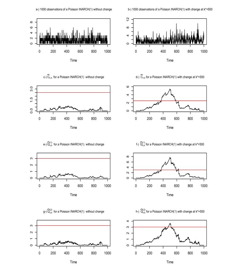
Figure 1: Typical realization of 1000 observations of two Poisson INGARCH(1) processes and the corresponding statistics $\widehat{C}^{(1)}_{n,k}$, $\widehat{Q}^{(1)}_{n,k}$ and $\widehat{Q}^{(2)}_{n,k}$. a-) is a Poisson INGARCH(1) process without change, where the parameter $\theta_{0}=(1,0.2)$ is constant. b-) is a Poisson INGARCH(1) process where the parameter $\theta_{0}=(1,0.2)$ changes to $(1,0.45)$ at $k^{*}=500$. c-), d-), e-), f-), g-) and h-) are their corresponding statistics $\widehat{C}_{n,k}$, $\widehat{Q}^{(1)}_{n,k}$ and $\widehat{Q}^{(2)}_{n,k}$. The horizontal line represents the limit of the critical region of the test.

One can see that, under H₀ the statistics $\widehat{C}_{n,k}$, $\widehat{Q}^{(1)}_{n,k}$ and $\widehat{Q}^{(2)}_{n,k}$ are below the horizontal line (see c-), e-), g-) ) which represents the limit of the critical region. These statistics are greater than the critical value in the neighborhood of the breakpoint under H₁ (see d-), f-), h-)). In several situations, only one of the statistics $\widehat{Q}^{(1)}_{n}$ and $\widehat{Q}^{(2)}_{n}$ is greater than the critical value under the alternative; so the use of $\widehat{Q}_{n}:=\max(\widehat{Q}_{n}^{(1)},\widehat{Q}_{n}^{(2)})$ is needed to get more powerful procedure.

5 Some simulations results

We provide some simulations results to show the empirical performance of these tests procedures. We consider a power Poisson INGARCH(1,1) :

$$Y_{t}/\mathcal{F}_{t-1}\sim\mbox{ Poisson}(\lambda_{t})~{}\text{with}~{}\lambda_{t}^{\delta}=\alpha_{0}+\alpha_{1}\lambda_{t-1}^{\delta}+\beta_{1}Y_{t-1}^{\delta}.$$ (13)

For a sample size $n=500,1000$, the statistics $\widehat{C}_{n}$ and $\widehat{Q}_{n}$ are computed with $u_{n}=v_{n}=[(\log n)^{5/2}]$. The empirical levels and powers reported in the followings table are obtained after 200 replications at the nominal level $\alpha=0.05$.

1. Poisson INGARCH(1,1) with one change-point alternative.
   We assume in (13) that $\delta=1$ and denote by $\theta=(\alpha_{0},\alpha_{1},\beta_{1})$ the parameter of the model. Table 1 indicates the empirical levels computed when the parameter is $\theta_{0}$ and the empirical powers computed when $\theta_{0}$ changes to $\theta_{1}$ at $n/2$.

   		Procedure	$n=500$	$n=1000$
   Empirical levels :	$\theta_{0}=(1,0.1,0.2)$	$\widehat{C}_{n}$ statistic	0.020	0.040
   		$\widehat{Q}_{n}$ statistic	0.035	0.045
   	$\theta_{0}=(0.3,0.5,0.1)$	$\widehat{C}_{n}$ statistic	0.065	0.060
   		$\widehat{Q}_{n}$ statistic	0.080	0.055
   Empirical powers :	$\theta_{0}=(1,0.1,0.2)$ ; $\theta_{1}=(0.7,0.1,0.2)$	$\widehat{C}_{n}$ statistic	0.415	0.840
   		$\widehat{Q}_{n}$ statistic	0.595	0.910
   	$\theta_{0}=(0.3,0.5,0.1)$ ; $\theta_{1}=(0.3,0.3,0.4)$	$\widehat{C}_{n}$ statistic	0.695	0.960
   		$\widehat{Q}_{n}$ statistic	0.865	0.995

   Table 1: Empirical levels and powers at the nominal level $0.05$ of test for parameter change in Poisson INGARCH(1,1) model with one change-point alternative.

2. Poisson INARCH(1) with two change-points alternative.
   We assume in (13) that $\delta=1$, $\alpha_{1}=0$ and denote by $\theta=(\alpha_{0},\beta_{1})$ the parameter of the model. Table 2 indicates the empirical levels computed when the parameter is $\theta_{0}$ and the empirical powers computed when $\theta_{0}$ changes to $\theta_{1}$ at $0.3n$ which changes to $\theta_{2}$ at $0.7n$.

   		Procedure	$n=500$	$n=1000$
   Empirical levels :	$\theta_{0}=(1,0.2)$	$\widehat{C}_{n}$ statistic	0.040	0.055
   		$\widehat{Q}_{n}$ statistic	0.065	0.035
   	$\theta_{0}=(0.2,0.5)$	$\widehat{C}_{n}$ statistic	0.080	0.050
   		$\widehat{Q}_{n}$ statistic	0.090	0.050
   Empirical powers :	$\theta_{0}=(1,0.2)$ ; $\theta_{1}=(1,0.45)$ ; $\theta_{2}=(1,0.15)$	$\widehat{C}_{n}$ statistic	0.715	0.955
   		$\widehat{Q}_{n}$ statistic	0.780	0.985
   	$\theta_{0}=(0.2,0.5)$ ; $\theta_{1}=(0.35,0.5)$ ; $\theta_{2}=(0.35,0.4)$	$\widehat{C}_{n}$ statistic	0.405	0.800
   		$\widehat{Q}_{n}$ statistic	0.540	0.865

   Table 2: Empirical levels and powers at the nominal level $0.05$ of test for parameter change in Poisson INARCH(1) model with two change-points alternative.

3. Power Poisson INGARCH(1) with one change-point alternative.
   We assume in (13) that $\delta=2$, $\alpha_{1}=0$ and denote by $\theta=(\alpha_{0},\beta_{1})$ the parameter of the model. Table 3 indicates the empirical levels computed when the parameter is $\theta_{0}$ and the empirical powers computed when $\theta_{0}$ changes to $\theta_{1}$ at $n/2$.

   		Procedure	$n=500$	$n=1000$
   Empirical levels :	$\theta_{0}=(0.8,0.15)$	$\widehat{C}_{n}$ statistic	0.020	0.045
   		$\widehat{Q}_{n}$ statistic	0.065	0.055
   Empirical powers :	$\theta_{0}=(0.8,0.15)$ ; $\theta_{1}=(1.3,0.15)$	$\widehat{C}_{n}$ statistic	0.415	0.870
   		$\widehat{Q}_{n}$ statistic	0.510	0.905
   	$\theta_{0}=(0.8,0.15)$ ; $\theta_{1}=(0.8,0.4)$	$\widehat{C}_{n}$ statistic	0.500	0.930
   		$\widehat{Q}_{n}$ statistic	0.590	0.945

   Table 3: Empirical levels and powers at the nominal level $0.05$ of test for parameter change in power Poisson INGARCH(1) model with one break alternative.

It appears in Table 1, 2, 3 that these two procedures produces a size distortion when $n=500$; but the empirical levels are close to the nominal one when $n=1000$. One can also see that the empirical powers of these procedures increase with $n$. Although the procedure based on $\widehat{Q}_{n}$ is little more powerful, the test based on $\widehat{C}_{n}$ provides satisfactory empirical powers even in the case of two change-points alternative. This will be the starting point to investigate in our future works, the consistency of this procedure under multiple change-points alternative.

6 Real data Application

We consider the number of transactions per minute for the stock Ericsson B during July 15, 2002. There are $460$ observations which represent trading from 09:35 to 17:14. Figure 2 plot the data and its autocorrelation function.

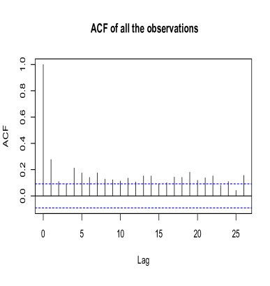
Figure 2: Number of transactions per minute for the stock Ericsson B during July 15, 2002 and their autocorrelation function.

Several works (see for instance Fokianos et al. [18], Davis and Liu [9]) on the series of July 2, 2002 led to use an INGARCH(1,1) model for this series. This model provides $\widehat{\alpha}_{1}+\widehat{\beta}_{1}$ close to unity. It can be seen in the slow decay of the autocorrelation function (see Figure 2). The authors saw a similarity with the high-persistence in IGARCH model. The series in the period 2-22 July 2002 have been studied by Brännäs and Quoreshi [5]. They have pointed out the presence of long memory in these data and applied INARMA model to both level and first difference forms.
To test the adequacy of the linearity of the transaction during July 15, 2002, we have applied the goodness-of-fit test for Poisson count processes proposed by Fokianos and Neumann [17]. Let $\widehat{\theta}_{n}=(\widehat{\alpha}_{0,n},\widehat{\alpha}_{1,n},\widehat{\beta}_{1,n})$ be the maximum likelihood estimator computed on the observations. Denote $\widehat{I}_{t}=(\widehat{\lambda}_{t},Y_{t})$ where $\widehat{\lambda}_{t}=\widehat{\alpha}_{0,n}+\widehat{\alpha}_{1,n}\widehat{\lambda}_{t-1}+\widehat{\beta}_{1,n}Y_{t-1}$. The estimated Pearson residuals is defined by $\widehat{\xi}_{t}=(Y_{t}-\widehat{\lambda}_{t})/\sqrt{\widehat{\lambda}_{t}}$. The goodness-of-fit test is based on the statistic

$$\widehat{T}_{n}=\sup_{x\in\Pi}|\widehat{G}_{n}(x)|~{}\text{ with }~{}\widehat{G}_{n}(x)=\frac{1}{\sqrt{n}}\sum_{t=1}^{n}\widehat{\xi}_{t}w(x-\widehat{I}_{t-1})$$

where $\Pi=[0,\infty)^{2}$ and $w(x)=w(x_{1},x_{2})=K(x_{1})K(x_{2})$ where $K(\cdot)$ is a univariate kernel. See [17] for more detail on this test procedure.
We have applied this test with uniform and Epanechnikov kernel and the p-values $0.032$ and $0.05$ have been obtained respectively. So, the linear assumption of the model is rejected. Recall that, Fokianos and Neumann [17] have already pointed out some doubt about the linearity assumption when they analyzed the series of 2 July 2002.
The previous test for change detection have been applied to the series of July 15, 2002. A change has been detected around the midday at $t^{*}=12:05$. Figure 3 shows the breakpoint and the autocorrelation function of each regime.

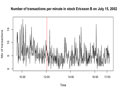
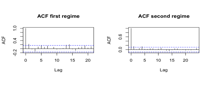
Figure 3: Breakpoint in transactions per minute for the stock Ericsson B and the autocorrelation function of each regime.

The previous goodness-of-fit test shows the adequacy of the linear Poisson autoregression of the first regime and raises some doubt about the linearity on the second regime. This shows that, the model structure of the transactions in the morning may be different to the structure of the transactions in the afternoon. Moreover, Figure 3 shows that the autocorrelation function of each regime decreases fast; this rules out the idea of the long memory in the series.

7 Proofs of the main results

Proof of the Proposition 2.1
We will use the same techniques as in [12]. Let $p,q$ two fixed non-negative integers. Definite the sequence $(\lambda_{t}^{p,q})_{t\in{\bf Z}}$ by

$$\lambda_{t}^{p,q}=\begin{cases}0&\text{if }t\leq-q\\ F(\lambda_{t-1}^{p,q},\ldots,\lambda_{t-p}^{p,q},0,\ldots;Y_{t-1},\ldots)&\text{ otherwise}.\end{cases}$$ (14)

The existence of moment of any order of the process $(Y_{t},\lambda_{t})_{t\in{\bf Z}}$ (see [13]) and assumption (A_F) imply the existence of moment of any order of $(\lambda_{t}^{p,q})_{t\in{\bf Z}}$. Let us show that $(\lambda_{0}^{p,q})_{q\geq 0}$ is a Cauchy sequence in $L^{1}$. By using (A_F), we have

$$E|\lambda_{0}^{p,q+1}-\lambda_{0}^{p,q}|\leq\sum\limits_{j=1}^{p}\alpha_{j}E|\lambda_{-j}^{p,q+1}-\lambda_{-j}^{p,q}|.$$

By definition and the strictly stationarity of $(Y_{t})_{t\in{\bf Z}}$, we can easily see that for $j=1\ldots,p$, the couples $(\lambda_{-j}^{p,q+1},\lambda_{-j}^{p,q+1})$ and $(\lambda_{0}^{p,q+1-j},\lambda_{0}^{p,q-j})$ have the same distribution. Hence, if comes that

$$E|\lambda_{0}^{p,q+1}-\lambda_{0}^{p,q}|\leq\sum\limits_{j=1}^{p}\alpha_{j}E|\lambda_{0}^{p,q+1-j}-\lambda_{0}^{p,q-j}|.$$

For any fixed $p$, denote $v_{q}=E|\lambda_{0}^{p,q+1}-\lambda_{0}^{p,q}|$ for all $q>p$. It holds that

$$v_{q}\leq\sum\limits_{j=1}^{p}\alpha_{j}v_{q-j}.$$

By applying the Lemma 5.4 of [12], we obtain

$$v_{q}\leq\alpha^{q/p}v_{0}\text{ where }\alpha=\sum\limits_{j=1}^{\infty}\alpha_{j}.$$

Hence, $v_{q}\rightarrow 0$ as $q\rightarrow\infty$. Thus, for any $p>0$, the sequence $(\lambda_{0}^{p,q})$ is a Cauchy sequence in $L^{1}$. Therefore, it converges to some limit denoted $\lambda_{0}^{p}$. Moreover, since the sequence $(\lambda_{0}^{p,q})_{q\geq 1}$ is measurable w.r.t to $\sigma(Y_{t},t<0)$, it is the case of the limit $\lambda_{0}^{p}$. So, there exists a measurable function $f^{(p)}$ such that $\lambda_{0}^{p}=f^{(p)}(Y_{-1},\ldots).$ By going along similar lines, it holds that for any $t\in{\bf Z}$, the sequence $(\lambda_{t}^{p,q})_{q\geq 1}$ converges in $L^{1}$ to some $\lambda_{t}^{p}=f^{(p)}(Y_{t-1},\ldots)$ and since $(Y_{t})_{t\in{\bf Z}}$, is stationary and ergodic, the process $(\lambda_{t}^{p})_{t\in{\bf Z}}$ is too stationary and ergodic.
Let $p$ and $t$ fixed. For $q$ large enough, $\lambda_{t}^{p,q}=F(\lambda_{t-1}^{p,q},\ldots,\lambda_{t-p}^{p,q},0,\ldots;Y_{t-1},\ldots)$ (see (14)). By using the continuity (which comes from Lipschitz-type conditions) of $(Y_{1},\ldots,Y_{p})\mapsto F(Y_{1},\ldots,Y_{p},0\ldots;y)$ for any fixed $y=(y_{1})_{i\geq 1}$ and by carrying $q$ to infinity, it holds that

$$\lambda_{t}^{p}=F(\lambda_{t-1}^{p},\ldots,\lambda_{t-p}^{p},0,\ldots;Y_{t-1},\ldots).$$ (15)

Denote $\mu_{p}=E\lambda_{t}^{p}$, $\mu=\underset{p\geq 1}{\sup}~{}\mu_{p}$, $\Delta_{p,t}=E|\lambda_{t}^{p+1}-\lambda_{t}^{p}|$ and $\Delta_{p}=\underset{t\in{\bf Z}}{\sup}\Delta_{p,t}$. By going the same lines as in [12], we obtain $\Delta_{p}\leq C\alpha_{p+1}$. Therefore, $\Delta_{p}\rightarrow 0$ as $p\rightarrow\infty$. This show that for any fixed $t\in{\bf Z}$, $(\lambda_{t}^{p})_{p\geq 1}$ is a Cauchy sequence in $L^{1}$. Thus it converges to some random $\widetilde{\lambda}_{t}\in L^{1}$. Moreover, $\widetilde{\lambda}_{t}$ is measurable w.r.t $\sigma(Y_{j},j<t)$ (because it is the case of $(\lambda_{t}^{p})_{p\geq 1}$). Thus, there exists a measurable function $f$ such that $\widetilde{\lambda}_{t}=f(Y_{t-1},\ldots)$ for any $t\in{\bf Z}$. This implies that $(\widetilde{\lambda}_{t})_{t\in{\bf Z}}$ is strictly stationary and ergodic. Finally, by using equation (15) and continuity of $F$, it comes that

$$\widetilde{\lambda}_{t}=F(\widetilde{\lambda}_{t-1},\ldots;Y_{t-1},\ldots)\text{ for any }t\in{\bf Z}.$$ (16)

Hence, the process $(Y_{t},\widetilde{\lambda}_{t})_{t\in{\bf Z}}$ is strictly stationary ergodic and satisfying (1). By the uniqueness of the solution, it holds that $\widetilde{\lambda}_{t}=\lambda_{t}$ a.s. Thus $\lambda_{t}=f(Y_{t-1},\ldots)$ for any $t\in{\bf Z}$.  

Proof of the Theorem 3.1

Without loss generality, for simplifying notation, we will make the proof with $T_{j_{n},k_{n}}=T_{1,n}$. It will follow two steps. We will first show that $\left\|\frac{1}{n}\sum_{t\in T_{1,n}}\widehat{\ell}_{t}(\theta)-L(\theta)\right\|_{\Theta}\xrightarrow[n\to+\infty]{a.s.}0$ where $L(\Theta):=E(\ell_{0}(\theta))$; secondly, we will show that the function $\theta\mapsto L(\Theta)$ has a unique maximum in $\theta_{0}$.

1. Let $\theta\in\Theta$, recall that $\ell_{t}(\theta)=Y_{t}\log\lambda_{t}(\theta)-\lambda_{t}(\theta)=Y_{t}\log f_{\theta}^{t}-f_{\theta}^{t}$. We have

   $$\left|\ell_{t}(\theta)\right| \leq\left|Y_{t}\right|\left|\log f_{\theta}^{t}\right|+\left|f_{\theta}^{t}\right|$$

   $$\leq\left|Y_{t}\right|\Big{|}\log\Big{(}\frac{f_{\theta}^{t}}{\underline{c}}\times\underline{c}\Big{)}\Big{|}+\left|f_{\theta}^{t}\right|$$

   $$\leq\left|Y_{t}\right|\Big{(}\Big{|}\frac{f_{\theta}^{t}}{c}-1\Big{|}+\left|\log\underline{c}\right|\Big{)}+\left|f_{\theta}^{t}\right|(\,\,\,\text{for}\,\,\,x>1,\left|\log x\right|\leq\left|x-1\right|)$$

   $$\leq\left|Y_{t}\right|\left(\frac{1}{\underline{c}}\left|f_{\theta}^{t}\right|+1+\left|\log\underline{c}\right|\right)+\left|f_{\theta}^{t}\right|.$$

   Hence,

   $$\sup_{\theta\in\Theta}\left|\ell_{t}(\theta)\right|\leq\left|Y_{t}\right|\Big{(}\frac{1}{\underline{c}}\left\|f_{\theta}^{t}\right\|_{\Theta}+1+\left|\log\underline{c}\right|\Big{)}+\left\|f_{\theta}^{t}\right\|_{\Theta}.$$

   We will show that, for any $r>0$, $E(\left\|f_{\theta}^{t}\right\|^{r}_{\Theta})<\infty$. Since A${}_{0}(\Theta)$ holds, we have

   $$\left\|f^{t}_{\theta}\right\|_{\Theta}\leq\left\|f^{t}_{\theta}-f_{\theta}(0)\right\|_{\Theta}+\left\|f_{\theta}(0)\right\|_{\Theta}\leq\sum_{j\geq 1}\alpha_{j}^{(0)}(\Theta)\left|Y_{t-j}\right|+\left\|f_{\theta}(0)\right\|_{\Theta}.$$

   Thus, by using the stationarity of the process $(Y_{t})_{t\in{\bf Z}}$, it follows that

   $$\Big{(}E\,(\left\|f^{t}_{\theta}\right\|_{\Theta}^{r})\Big{)}^{1/r}\leq\left\|Y_{0}\right\|^{r}\sum_{j\geq 1}\alpha_{j}^{(0)}(\Theta)+\left\|f_{\theta}(0)\right\|_{\Theta}<\infty.$$

   Therefore, we have

   $$E\Big{(}\sup_{\theta\in\Theta}\left|\ell_{t}(\theta)\right|\Big{)}\leq\frac{1}{\underline{c}}(E\left|Y_{t}\right|^{2})^{1/2}\cdot\left(E\left\|f_{\theta}^{t}\right\|^{2}_{\Theta}\right)^{1/2}+(1+\left|\log\underline{c}\right|)E\left|Y_{t}\right|+E\left\|f_{\theta}^{t}\right\|_{\Theta}<\infty.$$

   By the uniform strong law of large number applied on $(\ell_{t}(\theta))_{t\geq 1}$, it holds that

   $$\Big{\|}\frac{1}{n}\sum_{t\in T_{1,n}}\ell_{t}(\theta)-E\ell_{0}(\theta)\Big{\|}_{\Theta}\xrightarrow[n\to+\infty]{a.s.}0.$$ (17)

   Now let us show that

   $$\frac{1}{n}\Big{\|}\sum_{t\in T_{1,n}}\ell_{t}(\theta)-\sum_{t\in T_{1,n}}\widehat{\ell}_{t}(\theta)\Big{\|}_{\Theta}\xrightarrow[n\to+\infty]{a.s.}0.$$

   We have

   $$\frac{1}{n}\Big{\|}\sum_{t\in T_{1,n}}\ell_{t}(\theta)-\sum_{t\in T_{1,n}}\widehat{\ell}_{t}(\theta)\Big{\|}_{\Theta}\leq\frac{1}{n}\sum_{t\in T_{1,n}}\left\|\ell_{t}(\theta)-\widehat{\ell}_{t}(\theta)\right\|_{\Theta}.$$

   We will apply the Corollary $1$ of Kounias and Weng ($1969$). So, it suffices to show that

   $$\frac{1}{n}\sum_{t\geq 1}\frac{1}{t}E\Big{(}\left\|\ell_{t}(\theta)-\widehat{\ell}_{t}(\theta)\right\|_{\Theta}\Big{)}<\infty.$$

   For $t\in T_{1,n}$ and $\theta\in\Theta$, we have $\ell_{t}(\theta)-\widehat{\ell}_{t}(\theta)=Y_{t}\log f_{\theta}^{t}-f_{\theta}^{t}-Y_{t}\log\widehat{f}_{\theta}^{t}+\widehat{f}_{\theta}^{t}=Y_{t}(\log f_{\theta}^{t}-\log\widehat{f}_{\theta}^{t})-(f_{\theta}^{t}-\widehat{f}_{\theta}^{t})$.

   By using the relation $\left|\log f_{\theta}^{t}-\widehat{f}_{\theta}^{t}\right|\leq\frac{1}{\underline{c}}\left|f_{\theta}^{t}-\widehat{f}_{\theta}^{t}\right|$, it comes that

   $$\left\|\ell_{t}(\theta)-\widehat{\ell}_{t}(\theta)\right\|_{\Theta}\leq\frac{1}{\underline{c}}\left|Y_{t}\right|\left\|f_{\theta}^{t}-\widehat{f}_{\theta}^{t}\right\|_{\Theta}+\left\|f_{\theta}^{t}-\widehat{f}_{\theta}^{t}\right\|_{\Theta}\leq\Big{(}\frac{1}{\underline{c}}\left|Y_{t}\right|+1\Big{)}\left\|f_{\theta}^{t}-\widehat{f}_{\theta}^{t}\right\|.$$

   By Cauchy-Schwartz inequality,

   $$E\Big{(}\left\|\ell_{t}(\theta)-\widehat{\ell}_{t}(\theta)\right\|_{\Theta}\Big{)} \leq E\Big{[}\Big{(}\frac{1}{\underline{c}}\left|Y_{t}\right|+1\Big{)}\left\|f_{\theta}^{t}-\widehat{f}_{\theta}^{t}\right\|_{\Theta}\Big{]}$$

   $$\leq\Big{(}E\Big{(}\frac{1}{\underline{c}}\left|Y_{t}\right|+1\Big{)}^{2}\Big{)}^{1/2}\times\Big{(}E\left\|f_{\theta}^{t}-\widehat{f}_{\theta}^{t}\right\|^{2}_{\Theta}\Big{)}^{1/2}.$$

   We have (by Minkowski inequality),

   $$\Big{(}E\Big{(}\frac{1}{\underline{c}}\left|Y_{t}\right|+1\Big{)}^{2}\Big{)}^{1/2}\leq\frac{1}{\underline{c}}(E\left|Y_{t}\right|^{2})^{1/2}+1<\infty.$$

   Thus, it comes that

   $$E\Big{(}\left\|\ell_{t}(\theta)-\widehat{\ell}_{t}(\theta)\right\|_{\Theta}\Big{)}\leq C\Big{(}E\left\|f_{\theta}^{t}-\widehat{f}_{\theta}^{t}\right\|^{2}_{\Theta}\Big{)}^{1/2}.$$

   But, we have $\left\|f_{\theta}^{t}-\widehat{f}_{\theta}^{t}\right\|_{\Theta}\leq\sum_{j\geq t}\alpha_{j}^{(0)}(\Theta)\left|Y_{t-j}\right|$. By using Minkowski inequality, it comes that

   $$\Big{(}E\Big{\|}f_{\theta}^{t}-\widehat{f}_{\theta}^{t}\Big{\|}^{2}_{\Theta}\Big{)}^{1/2}\leq(E\,\left|Y_{0}\right|^{2})^{1/2}\sum_{j\geq t}\alpha_{j}^{(0)}(\Theta).$$

   Hence

   $$\Big{(}E\left\|f_{\theta}^{t}-\widehat{f}_{\theta}^{t}\right\|^{2}_{\Theta}\Big{)}^{1/2}\leq C\sum_{j\geq 0}\alpha_{j}^{(0)}(\Theta).$$

   Thus

   $$E\Big{(}\left\|\ell_{t}(\theta)-\widehat{\ell}_{t}(\theta)\right\|_{\Theta}\Big{)}\leq C\sum_{j\geq t}\alpha_{j}^{(0)}(\Theta).$$

   Therefore

   $$\sum_{t\geq 1}\frac{1}{t}E\left\|\ell_{t}(\theta)-\widehat{\ell}_{t}(\theta)\right\|_{\Theta} \leq C\sum_{t\geq 1}\frac{1}{t}\sum_{j\geq t}\alpha_{j}^{(0)}(\Theta)=C\sum_{t\geq 1}\sum_{j\geq t}\frac{1}{t}\alpha_{j}^{(0)}(\Theta)$$

   $$\leq\sum_{j\geq 1}\sum_{t=1}^{j}\frac{1}{t}\alpha_{j}^{(0)}(\Theta)=C\sum_{j\geq 1}\alpha_{j}^{(0)}(\Theta)\sum_{t=1}^{j}\frac{1}{t}$$

   $$\leq C\sum_{j=1}\alpha_{j}^{(0)}(\Theta)\cdot(1+\log j)$$

   $$\leq C\sum_{j\leq 1}\alpha_{j}^{(0)}(\Theta)+C\sum_{j\geq 1}\alpha_{j}^{(0)}(\Theta)\log j$$

   $$\leq 2C\sum_{j\geq 1}\alpha_{j}^{(0)}(\Theta)\log j<\infty.$$

   Hence, it follows that

   $$\frac{1}{n}\Big{\|}\sum_{t\in T_{1,n}}\ell_{t}(\theta)-\sum_{t\in T_{1,n}}\widehat{\ell}_{t}(\theta)\Big{\|}_{\Theta}\xrightarrow[n\to+\infty]{a.s.}0.$$ (18)

   From (17) and (18), we deduce that

   $$\Big{\|}\frac{1}{n}\sum_{t\in T_{1,n}}\widehat{\ell}_{t}(\theta)-E\ell_{0}(\theta)\Big{\|}_{\Theta}\xrightarrow[n\to\infty]{a.s.}0.$$

2. We will now show that the function $\theta\mapsto L(\theta)=E\ell_{0}(\theta)$ has a unique maximum at $\theta_{0}$. We will proceed as in [9]. Let $\theta\in\Theta$, with $\theta\neq\theta_{0}$. We have

   $$L(\theta_{0})-L(\theta) =E\ell_{0}(\theta_{0})-E\ell_{0}(\theta)$$

   $$=E(Y_{0}\log f_{\theta_{0}}^{0}-f_{\theta_{0}}^{0})-E(Y_{0}\log f_{\theta}^{0}-f_{\theta}^{0})$$

   $$=E\left[f_{\theta_{0}}^{0}(\log f_{\theta_{0}}^{0}-\log f_{\theta_{0}}^{0})\right]-E(f_{\theta_{0}}^{0}-f_{\theta_{0}}^{0}).$$

   By applying the mean value theorem at the function $x\mapsto\log x$ defined on $[\underline{c},+\infty[$, there exists $\xi$ between $f_{\theta_{0}}^{0}$ and $f_{\theta}^{0}$ such that $\log f_{\theta_{0}}^{0}-\log f_{\theta_{0}}^{0}=(f_{\theta_{0}}^{0}-f_{\theta_{0}}^{0})\frac{1}{\xi}$. Hence, it comes that

   $$L(\theta_{0})-L(\theta) =E\Big{(}\frac{1}{\xi}f_{\theta_{0}}^{0}(f_{\theta_{0}}^{0}-f_{\theta}^{0})\Big{)}-E(f_{\theta_{0}}^{0}-f_{\theta}^{0})$$

   $$=E\Big{(}\big{(}\frac{f_{\theta_{0}}^{0}}{\xi}-1\big{)}\big{(}f_{\theta_{0}}^{0}-f_{\theta}^{0}\big{)}\Big{)}$$

   $$=E\Big{(}\frac{1}{\xi}(f_{\theta_{0}}^{0}-\xi)(f_{\theta_{0}}^{0}-f_{\theta}^{0})\Big{)}.$$

   Since $\theta\neq\theta_{0}$, it follows from assumption $\mathrm{Id}(\Theta)$ that $\frac{1}{\xi}(f_{\theta_{0}}^{0}-\xi)(f_{\theta_{0}}^{0}-f_{\theta}^{0})\neq 0$ a.s. Moreover

   • if $f_{\theta_{0}}^{0}<f_{\theta}^{0}$, then $f_{\theta_{0}}^{0}<\xi<f_{\theta}^{0}$ and hence $\frac{1}{\xi}(f_{\theta_{0}}^{0}-\xi)(f_{\theta_{0}}^{0}-f_{\theta}^{0})>0$;

   • if $f_{\theta_{0}}^{0}>f_{\theta}^{0}$, then $f_{\theta}^{0}<\xi<f_{\theta_{0}}^{0}$ and hence $\frac{1}{\xi}(f_{\theta_{0}}^{0}-\xi)(f_{\theta_{0}}^{0}-f_{\theta}^{0})>0$.

   We deduce that $\frac{1}{\xi}(f_{\theta_{0}}^{0}-\xi)(f_{\theta_{0}}^{0}-f_{\theta}^{0})>0$ a.s.. Hence $L(\theta_{0})-L(\theta)=E\Big{(}\frac{1}{\xi}(f_{\theta_{0}}^{0}-\xi)(f_{\theta_{0}}^{0}-f_{\theta}^{0})\Big{)}>0$. Thus, the function $\theta\mapsto L(\theta)$ has a unique maximum at $\theta_{0}$.

(i), (ii) and standard arguments lead to the consistency of $\widehat{\theta}_{n}(T_{1,n})$.  

The following lemma is needed to prove the Theorem 3.2.

Lemma 7.1

Let $(j_{n})_{n\geq 1}$ and $(k_{n})_{n\geq 1}$ two integer valued sequences such that $(j_{n})_{n\geq 1}$ is increasing, $j_{n}\rightarrow\infty$ and $k_{n}-j_{n}\rightarrow\infty$ as $n\rightarrow\infty$. Let $n\geq 1$, for any segment $T=T_{j_{n},k_{n}}\subset\{1,\ldots,n\}$, it holds under assumptions of Theorem 3.2 that

• $E\,\Big{(}\dfrac{1}{\sqrt{k_{n}-j_{n}}}\Big{\|}\dfrac{\partial}{\partial\theta}L_{n}(T,\theta)-\dfrac{\partial}{\partial\theta}\widehat{L}_{n}(T,\theta)\Big{\|}_{\Theta}\Big{)}\underset{n\rightarrow\infty}{\longrightarrow 0}$ ;

• $\Big{\|}\dfrac{1}{k_{n}-j_{n}}\dfrac{\partial^{2}}{\partial\theta\partial\theta^{\prime}}L_{n}(T,\theta)-E\,\Big{(}\dfrac{\partial^{2}\ell_{0}(\theta)}{\partial\theta\partial\theta^{\prime}}\Big{)}\Big{\|}_{\Theta}\underset{n\rightarrow\infty}{\overset{a.s.}{\longrightarrow}0}$ ;

• $\Big{\|}\dfrac{1}{k_{n}-j_{n}}\sum_{t\in T}\dfrac{1}{\widehat{f}_{\theta}^{t}}\big{(}\dfrac{\partial}{\partial\theta}\widehat{f}_{\theta}^{t}\big{)}\big{(}\dfrac{\partial}{\partial\theta}\widehat{f}_{\theta}^{t}\big{)}^{\prime}-E\,\Big{(}\dfrac{1}{f^{0}_{\theta}}\big{(}\dfrac{\partial}{\partial\theta}f^{0}_{\theta}\big{)}\big{(}\dfrac{\partial}{\partial\theta}f^{0}_{\theta}\big{)}^{\prime}\Big{\|}_{\Theta}\underset{n\rightarrow\infty}{\overset{a.s.}{\longrightarrow}0}$.

Proof.

• Let $i\in\{1,\dots,n\}$. We have

  $$\frac{\partial}{\partial\theta_{i}}L_{n}(T,\theta)=\sum_{t\in T}\frac{\partial}{\partial\theta_{i}}(Y_{t}\log f_{\theta}^{t}-f_{\theta}^{t})=\sum_{t\in T}\left(Y_{t}\frac{1}{f_{\theta}^{t}}\frac{\partial}{\partial\theta_{i}}f_{\theta}^{t}-\frac{\partial}{\partial\theta_{i}}f_{\theta}^{t}\right)=\sum_{t\in T}\frac{\partial}{\partial\theta_{i}}\ell_{t}(\theta)$$

  and

  $$\frac{\partial}{\partial\theta_{i}}\widehat{L}_{n}(T,\theta)=\sum_{t\in T}\left(Y_{t}\frac{1}{\widehat{f}_{\theta}^{t}}\frac{\partial}{\partial\theta_{i}}\widehat{f}_{\theta}^{t}-\frac{\partial}{\partial\theta_{i}}\widehat{f}_{\theta}^{t}\right)=\sum_{t\in T}\frac{\partial}{\partial\theta_{i}}\widehat{\ell}_{t}(\theta).$$

  Hence

  $$\left|\frac{\partial}{\partial\theta_{i}}\ell_{t}(\theta)-\frac{\partial}{\partial\theta_{i}}\widehat{\ell}_{t}(\theta)\right| =\left|Y_{t}\frac{1}{f_{\theta}^{t}}\frac{\partial}{\partial\theta_{i}}f_{\theta}^{t}-\frac{\partial}{\partial\theta_{i}}f_{\theta}^{t}-Y_{t}\frac{1}{\widehat{f}_{\theta}^{t}}\frac{\partial}{\partial\theta_{i}}\widehat{f}_{\theta}^{t}+\frac{\partial}{\partial\theta_{i}}\widehat{f}_{\theta}^{t}\right|$$

  $$\leq\left|Y_{t}\right|\left|\frac{1}{f_{\theta}^{t}}\frac{\partial}{\partial\theta_{i}}f_{\theta}^{t}-\frac{1}{\widehat{f}_{\theta}^{t}}\frac{\partial}{\partial\theta_{i}}\widehat{f}_{\theta}^{t}\right|+\left|\frac{\partial}{\partial\theta_{i}}f_{\theta}^{t}-\frac{\partial}{\partial\theta_{i}}\widehat{f}_{\theta}^{t}\right|.$$ (19)

  Using the relation $\left|a_{1}b_{1}-a_{2}b_{2}\right|\leq\left|a_{1}-a_{2}\right|\left|b_{2}\right|+\left|b_{1}-b_{2}\right|\left|a_{1}\right|$, we have

  $$\left|\frac{1}{f_{\theta}^{t}}\frac{\partial}{\partial\theta_{i}}f_{\theta}^{t}-\frac{1}{\widehat{f}_{\theta}^{t}}\frac{\partial}{\partial\theta_{i}}\widehat{f}_{\theta}^{t}\right| \leq\left|\frac{1}{f_{\theta}^{t}}-\frac{1}{\widehat{f}_{\theta}^{t}}\right|\left|\frac{\partial}{\partial\theta_{i}}\widehat{f}_{\theta}^{t}\right|+\left|\frac{\partial}{\partial\theta_{i}}f_{\theta}^{t}-\frac{\partial}{\partial\theta_{i}}\widehat{f}_{\theta}^{t}\right|\left|\frac{1}{f_{\theta}^{t}}\right|$$

  $$\leq\frac{1}{\underline{c}^{2}}\left|f_{\theta}^{t}-\widehat{f}_{\theta}^{t}\right|\left|\frac{\partial}{\partial\theta_{i}}\widehat{f}_{\theta}^{t}\right|+\frac{1}{\underline{c}}\left|\frac{\partial}{\partial\theta_{i}}f_{\theta}^{t}-\frac{\partial}{\partial\theta_{i}}\widehat{f}_{\theta}^{t}\right|.$$

  Hence, (19) implies

  $$\left\|\frac{\partial}{\partial\theta_{i}}\ell_{t}(\theta)-\frac{\partial}{\partial\theta_{i}}\widehat{\ell}_{t}(\theta)\right\| \leq\left|Y_{t}\right|\left(\frac{1}{\underline{c}^{2}}\left\|f_{\theta}^{t}-\widehat{f}_{\theta}^{t}\right\|_{\Theta}\left\|\frac{\partial}{\partial\theta_{i}}\widehat{f}_{\theta}^{t}\right\|_{\Theta}+\frac{1}{\underline{c}}\left\|\frac{\partial}{\partial\theta_{i}}f_{\theta}^{t}-\frac{\partial}{\partial\theta_{i}}\widehat{f}_{\theta}^{t}\right\|_{\Theta}\right)+\left\|\frac{\partial}{\partial\theta_{i}}f_{\theta}^{t}-\frac{\partial}{\partial\theta_{i}}\widehat{f}_{\theta}^{t}\right\|_{\Theta}$$

  $$\leq C\left|Y_{t}\right|\left\|\frac{\partial}{\partial\theta_{i}}\widehat{f}_{\theta}^{t}\right\|_{\Theta}\left\|f_{\theta}^{t}-\widehat{f}_{\theta}^{t}\right\|_{\Theta}+C(1+\left|Y_{t}\right|)\left\|\frac{\partial}{\partial\theta_{i}}f_{\theta}^{t}-\frac{\partial}{\partial\theta_{i}}\widehat{f}_{\theta}^{t}\right\|_{\Theta}.$$

  Let $r>0$. Using the Minkowski and Hölder inequalities, it holds that

  $$\left(E\left[\left\|\frac{\partial}{\partial\theta_{i}}\ell_{t}(\theta)-\frac{\partial}{\partial\theta_{i}}\widehat{\ell}_{t}(\theta)\right\|^{r}_{\Theta}\right]\right)^{1/r} \leq C\left(E\left[\left|Y_{t}\right|^{r}\left\|\frac{\partial}{\partial\theta_{i}}\widehat{f}_{\theta}^{t}\right\|^{r}_{\Theta}\left\|f_{\theta}^{t}-\widehat{f}_{\theta}^{t}\right\|^{r}_{\Theta}\right]\right)^{1/r}$$

  $$\qquad+C\left(E\left[(1+\left|Y_{t}\right|)^{r}\left\|\frac{\partial}{\partial\theta_{i}}f_{\theta}^{t}-\frac{\partial}{\partial\theta_{i}}\widehat{f}_{\theta}^{t}\right\|^{r}_{\Theta}\right]\right)^{1/r}$$

  $$\leq C\left((E\left|Y_{t}\right|^{3r})^{1/3}\left(E\left\|\frac{\partial}{\partial\theta_{i}}\widehat{f}_{\theta}^{t}\right\|^{3r}_{\Theta}\right)^{1/3}\left(E\left\|f_{\theta}^{t}-\widehat{f}_{\theta}^{t}\right\|^{3r}_{\Theta}\right)^{1/3}\right)^{1/r}$$

  $$\qquad+C\left(\left(E(1+\left|Y_{t}\right|)^{2r}\right)^{1/r}\left(E\left\|\frac{\partial}{\partial\theta_{i}}f_{\theta}^{t}-\frac{\partial}{\partial\theta_{i}}\widehat{f}_{\theta}^{t}\right\|^{2r}\right)^{1/2}\right)^{1/r}$$

  $$\leq C\left\|Y_{t}\right\|_{3r}\left\|\left\|\frac{\partial}{\partial\theta_{i}}\widehat{f}_{\theta}^{t}\right\|_{\Theta}\right\|_{3r}\cdot\left(E\left\|f_{\theta}^{t}-\widehat{f}_{\theta}^{t}\right\|_{\Theta}^{3r}\right)^{1/3r}$$

  $$\qquad+C\left\|1+\left|Y_{t}\right|\right\|_{2r}\cdot\left(E\left\|\frac{\partial}{\partial\theta_{i}}f_{\theta}^{t}-\frac{\partial}{\partial\theta_{i}}\widehat{f}_{\theta}^{t}\right\|_{\Theta}^{2r}\right)^{1/2r}.$$

  But we have $\left\|Y_{t}\right\|_{3r}=C<\infty$ and $\left\|1+\left|Y_{t}\right|\right\|_{1r}<\infty$. Hence

  $$\left\|\frac{\partial}{\partial\theta_{i}}\widehat{f}_{\theta}^{t}\right\|_{\Theta}\leq\left\|\frac{\partial}{\partial\theta_{i}}f_{\theta}(0)\right\|_{\Theta}+\left\|\frac{\partial}{\partial\theta_{i}}\widehat{f}_{\theta}^{t}-\frac{\partial}{\partial\theta_{i}}f_{\theta}(0)\right\|_{\Theta}\leq C+\sum_{j\geq 1}\alpha_{j}^{(1)}(\Theta)\left|Y_{t-j}\right|.$$

  Thus,

  $$\left\|\left\|\frac{\partial}{\partial\theta_{i}}\widehat{f}_{\theta}^{t}\right\|_{\Theta}\right\|_{3r}\leq C+\left\|Y_{0}\right\|_{3r}\sum_{j\geq 1}\alpha_{j}^{(1)}(\Theta)\leq C(1+\sum_{j\geq 1}\alpha_{j}^{(1)}(\Theta))<\infty.$$

  We also have $\left\|f_{\theta}^{t}-\widehat{f}_{\theta}^{t}\right\|_{\Theta}\leq\sum_{j\geq t}\alpha_{j}^{(0)}(\Theta)\left|Y_{t-j}\right|$. Hence

  $$\left(E\left\|f_{\theta}^{t}-\widehat{f}_{\theta}^{t}\right\|^{3r}_{\Theta}\right)^{1/3r}=\left\|\left\|f_{\theta}^{t}-\widehat{f}_{\theta}^{t}\right\|_{\Theta}\right\|_{3r}\leq C\sum_{j\geq t}\alpha_{j}^{(0)}(\Theta).$$

  The same argument gives

  $$\left(E\left\|\frac{\partial}{\partial\theta_{i}}f_{\theta}^{t}-\frac{\partial}{\partial\theta_{i}}\widehat{f}_{\theta}^{t}\right\|^{2r}_{\Theta}\right)^{1/2r}=\left\|\left\|\frac{\partial}{\partial\theta_{i}}f_{\theta}^{t}-\frac{\partial}{\partial\theta_{i}}\widehat{f}_{\theta}^{t}\right\|_{\Theta}\right\|_{2r}\leq C\sum_{j\geq t}\alpha_{j}^{(1)}(\Theta).$$

  Hence,

  $$\left(E\left[\left\|\frac{\partial}{\partial\theta_{i}}\ell_{t}(\theta)-\frac{\partial}{\partial\theta_{i}}\widehat{\ell}_{t}(\theta)\right\|^{r}_{\Theta}\right]\right)^{1/r}\leq C\sum_{j\geq t}\left(\alpha_{j}^{(0)}(\Theta)+\alpha_{j}^{(1)}(\Theta)\right).$$

  Therefore, we have (with $r=1$)

  $$E\left(\frac{1}{\sqrt{k_{n}-j_{n}}}\left\|\frac{\partial}{\partial\theta_{i}}L_{n}(T,\theta)-\frac{\partial}{\partial\theta_{i}}\widehat{L}_{n}(T,\theta)\right\|_{\Theta}\right)\leq\frac{1}{\sqrt{k_{n}-j_{n}}}\sum_{t\in T}E\left\|\ell_{t}(\theta)-\widehat{\ell}_{t}(\theta)\right\|_{\Theta}$$

  $$\quad\leq C\frac{1}{\sqrt{k_{n}-j_{n}}}\sum_{t\in T}\left(\sum_{j\geq t}\left(\alpha_{j}^{(0)}(\Theta)+\alpha_{j}^{(1)}(\Theta)\right)\right)$$

  $$\quad\leq C\frac{1}{\sqrt{k_{n}-j_{n}}}\sum_{t\in T}\left[\sum_{j=t}^{k_{n}}\left(\alpha_{j}^{(0)}(\Theta)+\alpha_{j}^{(1)}(\Theta)\right)+\sum_{j\geq k_{n}}\left(\alpha_{j}^{(0)}(\Theta)+\alpha_{j}^{(1)}(\Theta)\right)\right]$$

  $$\quad\leq C\frac{1}{\sqrt{k_{n}-j_{n}}}\left[\sum_{t=j_{n}}^{k_{n}}\sum_{j=t}^{k_{n}}\left(\alpha_{j}^{(0)}(\Theta)+\alpha_{j}^{(1)}(\Theta)\right)+\sum_{t=j_{n}}^{k_{n}}\sum_{j\geq k_{n}}\left(\alpha_{j}^{(0)}(\Theta)+\alpha_{j}^{(1)}(\Theta)\right)\right]$$

  $$\quad\leq C\frac{1}{\sqrt{k_{n}-j_{n}}}\left[\sum_{j=j_{n}}^{k_{n}}\sum_{t=j_{n}}^{j}\left(\alpha_{j}^{(0)}(\Theta)+\alpha_{j}^{(1)}(\Theta)\right)+(k_{n}-j_{n})\sum_{j\geq k_{n}}\left(\alpha_{j}^{(0)}(\Theta)+\alpha_{j}^{(1)}(\Theta)\right)\right]$$

  $$\quad\leq C\frac{1}{\sqrt{k_{n}-j_{n}}}\left[\sum_{j=j_{n}}^{k_{n}}(j-j_{n})\left(\alpha_{j}^{(0)}(\Theta)+\alpha_{j}^{(1)}(\Theta)\right)+(k_{n}-j_{n})\sum_{j\geq k_{n}}\left(\alpha_{j}^{(0)}(\Theta)+\alpha_{j}^{(1)}(\Theta)\right)\right]$$

  $$\quad\leq C\frac{1}{\sqrt{k_{n}-j_{n}}}\sum_{j=j_{n}}^{k_{n}}(j-j_{n})\left(\alpha_{j}^{(0)}(\Theta)+\alpha_{j}^{(1)}(\Theta)\right)+C\sqrt{k_{n}-j_{n}}\sum_{j\geq k_{n}}\left(\alpha_{j}^{(0)}(\Theta)+\alpha_{j}^{(1)}(\Theta)\right)$$

  $$\quad\leq\frac{C}{\sqrt{k_{n}-j_{n}}}\sum_{j=j_{n}}^{j_{n}+\log(k_{n}-j_{n})}(j-j_{n})\left(\alpha_{j}^{(0)}(\Theta)+\alpha_{j}^{(1)}(\Theta)\right)$$

  $$\qquad+\frac{C}{\sqrt{k_{n}-j_{n}}}\sum_{j=j_{n}+\log(k_{n}-j_{n})}^{k_{n}}(j-j_{n})\left(\alpha_{j}^{(0)}(\Theta)+\alpha_{j}^{(1)}(\Theta)\right)+C\sum_{j\geq k_{n}}\sqrt{j}\left(\alpha_{j}^{(0)}(\Theta)+\alpha_{j}^{(1)}(\Theta)\right)$$

  $$\quad\leq\frac{C\log(k_{n}-j_{n})}{\sqrt{k_{n}-j_{n}}}\sum_{j\geq 1}\left(\alpha_{j}^{(0)}(\Theta)+\alpha_{j}^{(1)}(\Theta)\right)+C\sum_{j\geq j_{n}+\log(k_{n}-j_{n})}\sqrt{j-j_{n}}\left(\alpha_{j}^{(0)}(\Theta)+\alpha_{j}^{(1)}(\Theta)\right)$$

  $$\qquad+C\sum_{j\geq k_{n}}\sqrt{j}\left(\alpha_{j}^{(0)}(\Theta)+\alpha_{j}^{(1)}(\Theta)\right)$$

  $$\qquad\qquad\qquad\xrightarrow[n\to+\infty]{}0.$$

  This holds for any coordinate $i=1\dots,d$. This (i) has been proved.

• For $i,j\in\{1,\ldots,d\}$, we have

  $$\frac{\partial^{2}}{\partial\theta_{i}\partial\theta_{j}}\ell_{t}(\theta) =\frac{\partial}{\partial\theta_{j}}(Y_{t}\frac{1}{f_{\theta}^{t}}\frac{\partial}{\partial\theta_{i}}f_{\theta}^{t}-\frac{\partial}{\partial\theta_{i}}f_{\theta}^{t})$$

  $$=Y_{t}\left[\frac{\partial}{\partial\theta_{j}}\left(\frac{1}{f_{\theta}^{t}}\right)\times\frac{\partial}{\partial\theta_{i}}f_{\theta}^{t}+\frac{1}{f_{\theta}^{t}}\times\frac{\partial^{2}}{\partial\theta_{i}\partial\theta_{j}}f_{\theta}^{t}\right]-\frac{\partial^{2}}{\partial\theta_{i}\partial\theta_{j}}f_{\theta}^{t}$$

  $$=Y_{t}\left[-\frac{1}{\left(f_{\theta}^{t}\right)^{2}}\left(\frac{\partial}{\partial\theta_{j}}f_{\theta}^{t}\right)\times\frac{\partial}{\partial\theta_{i}}f_{\theta}^{t}+\frac{1}{f_{\theta}^{t}}\times\frac{\partial^{2}}{\partial\theta_{i}\partial\theta_{j}}f_{\theta}^{t}\right]-\frac{\partial^{2}}{\partial\theta_{i}\partial\theta_{j}}f_{\theta}^{t}$$

  $$=-\frac{Y_{t}}{\left(f_{\theta}^{t}\right)^{2}}\left(\frac{\partial}{\partial\theta_{i}}f_{\theta}^{t}\right)\left(\frac{\partial}{\partial\theta_{j}}f_{\theta}^{t}\right)+\left(\frac{Y_{t}}{f_{\theta}^{t}}-1\right)\frac{\partial^{2}}{\partial\theta_{i}\partial\theta_{j}}f_{\theta}^{t}.$$ (20)

  We will show that $E\left[\left\|\frac{\partial^{2}}{\partial\theta_{i}\partial\theta_{j}}\ell_{t}(\theta)\right\|\right]<+\infty$. We have

  $$E\left[\left\|\frac{\partial^{2}}{\partial\theta_{i}\partial\theta_{j}}\ell_{t}(\theta)\right\|_{\Theta}\right] \leq\frac{1}{\underline{c}^{2}}E\left[\left|Y_{t}\right|\left\|\frac{\partial}{\partial\theta_{i}}f_{\theta}^{t}\right\|_{\Theta}\left\|\frac{\partial}{\partial\theta_{j}}f_{\theta}^{t}\right\|_{\Theta}\right]+E\left[\left(\frac{\left|Y_{t}\right|}{\underline{c}}+1\right)\left\|\frac{\partial^{2}}{\partial\theta_{i}\partial\theta_{j}}f_{\theta}^{t}\right\|_{\Theta}\right]$$

  $$\leq C\left\|Y_{t}\right\|_{3}\left\|\left\|\frac{\partial}{\partial\theta_{i}}f_{\theta}^{t}\right\|_{\Theta}\left\|\frac{\partial}{\partial\theta_{j}}f_{\theta}^{t}\right\|_{\Theta}\right\|_{3}+C(\left\|Y_{t}\right\|_{2}+1)\left\|\left\|\frac{\partial^{2}}{\partial\theta_{i}\partial\theta_{j}}f_{\theta}^{t}\right\|_{\Theta}\right\|_{2}.$$

  But, we have $\left\|Y_{t}\right\|_{3}=\left\|Y_{0}\right\|_{3}<\infty$, and $\left\|Y_{t}\right\|_{2}<\infty$.

  $$\left\|\left\|\frac{\partial}{\partial\theta_{i}}f_{\theta}^{t}\right\|_{\theta}\right\|_{3} \leq\left\|\left\|\frac{\partial}{\partial\theta_{i}}f_{\theta}(0)\right\|_{\Theta}\right\|_{3}+\left\|\left\|\frac{\partial}{\partial\theta_{i}}f_{\theta}^{t}-\frac{\partial}{\partial\theta_{i}}f_{\theta}(0)\right\|_{\Theta}\right\|_{3}$$

  $$\leq\left\|\frac{\partial}{\partial\theta_{i}}f_{\theta}(0)\right\|_{\Theta}+\left\|\sum_{j\geq 1}\alpha_{j}^{(1)}(\Theta)\left|Y_{t-j}\right|\right\|_{3}$$

  $$\leq\left\|\frac{\partial}{\partial\theta_{i}}f_{\theta}^{t}\right\|_{\Theta}+\left\|Y_{0}\right\|_{3}\sum_{j\geq 1}\alpha_{j}^{(1)}(\Theta)<+\infty.$$

  Similarly, we have $\left\|\left\|\frac{\partial}{\partial\theta_{j}}f_{\theta}^{t}\right\|_{\Theta}\right\|_{3}<+\infty$. Using the same argument, we obtain

  $$\left\|\left\|\frac{\partial^{2}}{\partial\theta_{i}\partial\theta_{j}}f_{\theta}^{t}\right\|_{\Theta}\right\|_{2}\leq\left\|Y_{0}\right\|_{2}\sum_{j\geq 1}\alpha_{j}^{(2)}(\Theta)<+\infty.$$

  Hence, $E\left[\left\|\frac{\partial^{2}}{\partial\theta_{i}\partial\theta_{j}}\ell_{t}(\theta)\right\|_{\Theta}\right]<+\infty$. Thus, for the stationary ergodicity of the sequence $\left(\frac{\partial^{2}}{\partial\theta_{i}\partial\theta_{j}}\ell_{t}(\theta)\right)_{t\in{\bf Z}}$ and the uniform strong law of large numbers, it holds that

  $$\left\|\frac{1}{k_{n}-j_{n}}\frac{\partial^{2}}{\partial\theta_{i}\partial\theta_{j}}\ell_{t}(\theta)-E\frac{\partial^{2}}{\partial\theta_{i}\partial\theta_{j}}\ell_{0}(\theta)\right\|_{\Theta}\xrightarrow[n\to+\infty]{a.s.}0.$$

  This completes the proof of (ii).

• Goes the same lines as in (i) and (ii).

 

Proof of Theorem 3.2

Here again, without loss generality we will make the proof with $T_{j_{n},k_{n}}=T_{1,n}$. Recall that $\Theta\subset I\!\!R^{d}$. Let $T\subset\{1,\ldots,n\}$; for any $\overline{\theta}\in\Theta$ and $i=1,\ldots,n$, by applying the Taylor expansion to the function $\theta\mapsto\frac{\partial}{\partial\theta}L_{n}(T,\theta)$, there exists $\theta_{n,i}$ between $\overline{\theta}$ and $\theta_{0}$ such that

$$\frac{\partial}{\partial\theta_{i}}L_{n}(T,\overline{\theta})=\frac{\partial}{\partial\theta_{i}}L_{n}(T,\theta_{0})+\frac{\partial^{2}}{\partial\theta\partial\theta_{i}}L_{n}(T,\theta_{n,i})\cdot(\overline{\theta}-\theta_{0}).$$

Denote

$$G_{n}(T,\overline{\theta})=-\frac{1}{Card(T)}\Big{(}\frac{\partial^{2}}{\partial\theta\partial\theta_{i}}L_{n}(T,\theta_{n,i})\Big{)}_{1\leq i\leq d}.$$

It comes that

$$Card(T)G_{n}(T,\overline{\theta})\cdot(\overline{\theta}-\theta_{0})=\frac{\partial}{\partial\theta}L_{n}(T,\theta_{0})-\frac{\partial}{\partial\theta}L_{n}(T,\overline{\theta}).$$ (21)

By applying (21) with $\overline{\theta}=\widehat{\theta}_{n}(T)$ we obtain

$$Card(T)G_{n}(T,\widehat{\theta}_{n}(T))\cdot(\widehat{\theta}_{n}(T)-\theta_{0})=\frac{\partial}{\partial\theta}L_{n}(T,\theta_{0})-\frac{\partial}{\partial\theta}L_{n}(T,\widehat{\theta}_{n}(T)).$$ (22)

(22) holds for any $T\subset\{1,\ldots,n\}$, thus

$$\sqrt{n}G_{n}(T_{1,n},\widehat{\theta}_{n}(T_{1,n}))\cdot(\widehat{\theta}_{n}(T_{1,n})-\theta_{0})=\frac{1}{\sqrt{n}}\Big{(}\frac{\partial}{\partial\theta}L_{n}(T_{1,n},\theta_{0})-\frac{\partial}{\partial\theta}L_{n}(T_{1,n},\widehat{\theta}_{n}(T_{1,n}))\Big{)}.$$ (23)

We can rewrite (23) as

$$\sqrt{n}G_{n}(T_{1,n},\widehat{\theta}_{n}(T_{1,n}))(\widehat{\theta}_{n}(T_{1,n})-\theta_{0}) =\frac{1}{\sqrt{n}}\frac{\partial}{\partial\theta}L_{n}(T_{1,n},\theta_{0})-\frac{1}{\sqrt{n}}\frac{\partial}{\partial\theta}\widehat{L}_{n}(T_{1,n},\widehat{\theta}_{n}(T_{1,n}))$$

$$\qquad+\frac{1}{\sqrt{n}}\left(\frac{\partial}{\partial\theta}\widehat{L}_{n}(T_{1,n},\widehat{\theta}_{n}(T_{1,n}))-\frac{\partial}{\partial\theta}L_{n}(T_{1,n},\widehat{\theta}_{n}(T_{1,n}))\right).$$

For $n$ large enough, $\frac{\partial}{\partial\theta}\widehat{L}_{n}(T_{1,n},\widehat{\theta}_{n}(T_{1,n}))=0$, because $\widehat{\theta}_{n}(T_{1,n})$ is a local maximum of $\theta\mapsto\widehat{L}(T_{1,n},\theta)$. Moreover, according to Lemma 7.1 (i), it holds that

$$E\left(\frac{1}{\sqrt{n}}\left|\frac{\partial}{\partial\theta}L_{n}(T_{1,n},\widehat{\theta}_{n}(T_{1,n}))-\frac{\partial}{\partial\theta}\widehat{L}_{n}(T_{1,n},\widehat{\theta}_{n}(T_{1,n}))\right|\right) \leq E\left(\frac{1}{\sqrt{n}}\left\|\frac{\partial}{\partial\theta}L_{n}(T_{1,n},\theta)-\frac{\partial}{\partial\theta}\widehat{L}_{n}(T_{1,n},\theta)\right\|_{\Theta}\right)$$

$$\qquad\xrightarrow[n\to+\infty]{}0.$$

So, for $n$ large enough, we have

$$\sqrt{n}G_{n}(T_{1,n},\widehat{\theta}_{n}(T_{1,n}))(\widehat{\theta}_{n}(T_{1,n})-\theta_{0})=\frac{1}{\sqrt{n}}\frac{\partial}{\partial\theta}L_{n}(T_{1,n},\theta_{0})+o_{P}(1).$$ (24)

To complete the proof of Theorem 3.2, we have to show that

1. $\left(\frac{\partial}{\partial\theta}\ell_{t}(\theta_{0}),\mathcal{F}_{t}\right)_{t\in{\bf Z}}$ is a stationary ergodic martingable difference sequence and $E\left(\left\|\frac{\partial}{\partial\theta}\ell_{t}(\theta_{0})\right\|^{2}\right)<\infty$;

2. $\Sigma=-E\left(\frac{\partial^{2}}{\partial\theta\partial\theta^{\prime}}\ell_{0}(\theta_{0})\right)$ and $G_{n}(T_{1,n},\widehat{\theta}_{n}(T_{1,n}))\xrightarrow[n\to+\infty]{a.s.}\Sigma$;

3. $\Sigma=E\Big{[}\frac{1}{f^{0}_{\theta_{0}}}\left(\frac{\partial}{\partial\theta}f^{0}_{\theta_{0}}\right)\left(\frac{\partial}{\partial\theta}f^{0}_{\theta_{0}}\right)^{\prime}\Big{]}$ is invertible.

1. Recall that $\frac{\partial}{\partial\theta}\ell_{t}(\theta_{0})=\left(\frac{Y_{t}}{f_{\theta_{0}}^{t}}-1\right)\frac{\partial}{\partial\theta}f_{\theta_{0}}^{t}$ and $\mathcal{F}_{t}=\sigma(Y_{s},s\leq t)$. Since the functions $f_{\theta_{0}}^{t}$ and $\frac{\partial}{\partial\theta}f_{\theta_{0}}^{t}$ are $\mathcal{F}_{t-1}$-measurable, we have

   $$E\Big{(}\frac{\partial}{\partial\theta}\ell_{t}(\theta_{0})\big{|}\mathcal{F}_{t-1}\Big{)}=\Big{(}\frac{1}{f_{\theta_{0}}^{t}}E(Y_{t}|\mathcal{F}_{t-1})-1\Big{)}\frac{\partial}{\partial\theta}f_{\theta_{0}}^{t}=0.$$

   Moreover, since $\left|Y_{t}\right|$ and $\left\|\frac{\partial}{\partial\theta}f_{\theta}^{t}\right\|$ have moment of any order, we have

   $$E\Big{(}\big{|}\frac{\partial}{\partial\theta}\ell_{t}(\theta_{0})\big{|}^{2}\Big{)}\leq E\Big{(}\big{(}\frac{\left|Y_{t}\right|}{\underline{c}}+1\big{)}^{2}\big{\|}\frac{\partial}{\partial\theta}f_{\theta}^{t}\big{\|}^{2}_{\Theta}\Big{)}<\infty.$$

2. According to (20), we have

   $$\dfrac{\partial^{2}}{\partial\theta\partial\theta^{\prime}}\ell_{t}(\theta)=-\dfrac{Y_{t}}{\Big{(}f_{\theta}^{t}\Big{)}^{2}}\Big{(}\frac{\partial}{\partial\theta}f_{\theta}^{t}\Big{)}\Big{(}\frac{\partial}{\partial\theta}f_{\theta}^{t}\Big{)}^{\prime}+\Big{(}\dfrac{Y_{t}}{f_{\theta}^{t}}-1\Big{)}\dfrac{\partial^{2}}{\partial\theta\partial\theta^{\prime}}f_{\theta}^{t}.$$ (25)

   But by using the same argument as in (a), we obtain $E\,\Big{(}\big{(}\dfrac{Y_{t}}{f^{0}_{\theta_{0}}}-1\big{)}\dfrac{\partial^{2}}{\partial\theta\partial\theta^{\prime}}f^{0}_{\theta_{0}}\big{|}\mathcal{F}_{t-1}\Big{)}=0$. Hence, (25) implies

   $$E\,\Big{(}\dfrac{\partial^{2}}{\partial\theta\partial\theta^{\prime}}\ell_{t}(\theta_{0})\Big{)}=-E\,\left(\dfrac{Y_{t}}{(f^{0}_{\theta_{0}})^{2}}\Big{(}\frac{\partial}{\partial\theta}f^{0}_{\theta_{0}}\Big{)}\Big{(}\frac{\partial}{\partial\theta}f^{0}_{\theta_{0}}\Big{)}^{\prime}\right)=-E\,\left(\dfrac{1}{f^{0}_{\theta_{0}}}\Big{(}\frac{\partial}{\partial\theta}f^{0}_{\theta_{0}}\Big{)}\Big{(}\frac{\partial}{\partial\theta}f^{0}_{\theta_{0}}\Big{)}^{\prime}\right)=-\Sigma.$$

   Moreover, recall that

   $$G_{n}(T_{1,n},\widehat{\theta}_{n}(T_{1,n}))=-\frac{1}{n}\left(\frac{\partial^{2}}{\partial\theta\partial\theta_{i}}L(T_{1,n},\theta_{n,i})\right)_{1\leq i\leq d}\\ =-\frac{1}{n}\left(\sum_{t=1}^{n}\frac{\partial^{2}}{\partial\theta\partial\theta_{i}}\ell_{t}(\theta_{n,i})\right)_{1\leq i\leq d}.$$

   For any $j=1,\dots,d$, we have

   $$\left|\frac{1}{n}\sum_{t=1}^{n}\frac{\partial^{2}}{\partial\theta_{j}\partial\theta_{i}}\ell_{t}(\theta_{n,i})-E\left(\frac{\partial^{2}}{\partial\theta_{j}\partial\theta_{i}}\ell_{0}(\theta_{0})\right)\right| \leq\left|\frac{1}{n}\sum_{t=1}^{n}\frac{\partial^{2}}{\partial\theta_{j}\partial\theta_{i}}\ell_{t}(\theta_{n,i})-E\left(\frac{\partial^{2}}{\partial\theta_{j}\partial\theta_{i}}\ell_{0}(\theta_{n,i})\right)\right|$$

   $$\qquad+\left|E\left(\frac{\partial^{2}}{\partial\theta_{j}\partial\theta_{i}}\ell_{0}(\theta_{n,i})\right)-E\left(\frac{\partial^{2}}{\partial\theta_{j}\partial\theta_{i}}\ell_{0}(\theta_{0})\right)\right|$$

   $$\leq\left|E\left(\frac{\partial^{2}}{\partial\theta_{j}\partial\theta_{i}}\ell_{0}(\theta_{n,i})\right)-E\left(\frac{\partial^{2}}{\partial\theta_{j}\partial\theta_{i}}\ell_{0}(\theta_{0})\right)\right|$$

   $$\qquad+\left\|\frac{1}{n}\sum_{t=1}^{n}\frac{\partial^{2}}{\partial\theta_{j}\partial\theta_{i}}\ell_{t}(\theta)-E\left(\frac{\partial^{2}}{\partial\theta_{j}\partial\theta_{i}}\ell_{0}(\theta)\right)\right\|_{\Theta}$$

   $$\quad\xrightarrow[n\to+\infty]{a.s.}0.$$

   This holds for any $1\leq i,j\leq d$. Thus,

   $$G_{n}(T_{1,n},\widehat{\theta}_{n}(T_{1,n})) =-\frac{1}{n}\left(\frac{\partial^{2}}{\partial\theta\partial\theta_{i}}\ell_{t}(\theta_{n,i})\right)_{1\leq i\leq d}$$

   $$\xrightarrow[n\to+\infty]{a.s.}-E\left(\frac{\partial^{2}}{\partial\theta\partial\theta^{\prime}}\ell_{0}(\theta_{0})\right)=E\left[\frac{1}{f_{\theta_{0}}^{0}}\left(\frac{\partial}{\partial\theta}f_{\theta_{0}}^{0}\right)\left(\frac{\partial}{\partial\theta}f_{\theta_{0}}^{0}\right)^{\prime}\right]=\Sigma.$$

3. If $U$ is a non-zero vector of $I\!\!R^{d}$, according to assumption Var, it holds that $U\frac{\partial}{\partial\theta}f_{\theta_{0}}^{0}\neq 0$ a.s. Hence

   $$U\Sigma U^{\prime}=E\left(\frac{1}{f_{\theta_{0}}^{0}}U\left(\frac{\partial}{\partial\theta}f^{0}_{\theta_{0}}\right)\left(\frac{\partial}{\partial\theta}f^{0}_{\theta_{0}}\right)^{\prime}U^{\prime}\right)>0.$$

   Thus $\Sigma$ is positive definite.

From (a), apply the central limit theorem for stationary ergodic martingable difference sequence, it follows that

$$\frac{1}{\sqrt{n}}\frac{\partial}{\partial\theta}L_{n}(T_{1,n},\theta_{0})=\frac{1}{\sqrt{n}}\sum_{t=1}^{n}\frac{\partial}{\partial\theta}\ell_{t}(\theta_{0})\xrightarrow[n\to+\infty]{\mathcal{D}}\mathcal{N}\left(0,E\left[\left(\frac{\partial}{\partial\theta}\ell_{0}(\theta_{0})\right)\left(\frac{\partial}{\partial\theta}\ell_{0}(\theta_{0})\right)^{\prime}\right]\right).$$ (26)

Recall that for $i=1,\dots,d$, $\frac{\partial}{\partial\theta_{i}}\ell_{t}(\theta)=\left(\frac{Y_{t}}{f_{\theta}^{t}}-1\right)\frac{\partial}{\partial\theta_{i}}f_{\theta}^{t}$. For $1\leq i,j\leq d$, we have

$$E\Big{(}\frac{\partial}{\partial\theta_{i}}\ell_{t}(\theta_{0})\times\frac{\partial}{\partial\theta_{j}}\ell_{t}(\theta_{0})\Big{)} =E\Big{[}E\Big{(}\big{(}\frac{Y_{t}}{f_{\theta_{0}}^{t}}-1\big{)}^{2}\frac{\partial}{\partial\theta_{i}}f_{\theta_{0}}^{t}\times\frac{\partial}{\partial\theta_{j}}f_{\theta_{0}}^{t}\big{|}\mathcal{F}_{t-1}\Big{)}\Big{]}$$

$$=E\Big{[}E\Big{(}\big{(}\frac{Y_{t}}{f_{\theta_{0}}^{t}}-1\big{)}^{2}\big{|}\mathcal{F}_{t-1}\Big{)}\times\frac{\partial}{\partial\theta_{i}}f_{\theta_{0}}^{t}\times\frac{\partial}{\partial\theta_{j}}f_{\theta_{0}}^{t}\Big{]}$$

But, we have,

$$E\Big{[}\Big{(}\frac{Y_{t}}{f_{\theta_{0}}^{t}}-1\Big{)}^{2}\big{|}\mathcal{F}_{t-1}\Big{]} =\frac{1}{(f_{\theta_{0}}^{t})^{2}}E(Y_{t}^{2}|\mathcal{F}_{t-1})-\frac{2}{f_{\theta_{0}}^{t}}\times f_{\theta_{0}}^{t}+1=\frac{1}{(f_{\theta_{0}}^{t})^{2}}E(Y_{t}^{2}|\mathcal{F}_{t-1})-1$$

$$=\frac{1}{(f_{\theta_{0}}^{t})^{2}}\Big{(}\mbox{Var}\hskip 1.13809pt(Y_{t}|\mathcal{F}_{t-1})+(E(Y_{t}|\mathcal{F}_{t-1}))^{2}\Big{)}-1=\frac{1}{(f_{\theta_{0}}^{t})^{2}}(f_{\theta_{0}}^{t}+(f_{\theta_{0}}^{t})^{2})-1=\frac{1}{f_{\theta_{0}}^{t}}.$$

It comes that,

$$E\Big{[}\Big{(}\frac{\partial}{\partial\theta_{i}}\ell_{t}(\theta_{0})\Big{)}\times\Big{(}\frac{\partial}{\partial\theta_{j}}\ell_{t}(\theta_{0})\Big{)}^{\prime}\Big{]}=E\Big{[}\frac{1}{f_{\theta_{0}}^{t}}\Big{(}\frac{\partial}{\partial\theta_{i}}f_{\theta_{0}}^{t}\Big{)}\times\Big{(}\frac{\partial}{\partial\theta_{j}}f_{\theta_{0}}^{t}\Big{)}^{\prime}\Big{]}.$$

Hence

$$E\Big{[}\Big{(}\frac{\partial}{\partial\theta}\ell_{t}(\theta_{0})\Big{)}\times\Big{(}\frac{\partial}{\partial\theta}\ell_{t}(\theta_{0})\Big{)}^{\prime}\Big{]}=E\Big{[}\frac{1}{f_{\theta_{0}}^{t}}\Big{(}\frac{\partial}{\partial\theta}f_{\theta_{0}}^{t}\Big{)}\times\Big{(}\frac{\partial}{\partial\theta}f_{\theta_{0}}^{t}\Big{)}^{\prime}\Big{]}=\Sigma.$$

Thus, (26) becomes

$$\frac{1}{\sqrt{n}}\frac{\partial}{\partial\theta}L_{n}(T_{1,n},\theta_{0})=\frac{1}{\sqrt{n}}\sum_{t=1}^{n}\frac{\partial}{\partial\theta}\ell_{t}(\theta_{0})\xrightarrow[n\to+\infty]{\mathcal{D}}\mathcal{N}(0,\Sigma).$$ (27)

(b) and (c) implies that the matrix $G_{n}(T_{1,n},\widehat{\theta}_{n}(T_{1,n}))$ converges a.s. to $\Sigma$ and $G_{n}(T_{1,n},\widehat{\theta}_{n}(T_{1,n}))$ is invertible for $n$ large enough. Hence, from (24) and (27), we have

$$\sqrt{n}(\widehat{\theta}_{n}(T_{1,n})-\theta_{0}) =\frac{1}{\sqrt{n}}\left(G_{n}(T_{1,n},\widehat{\theta}_{n}(T_{1,n}))\right)^{-1}\frac{\partial}{\partial\theta}L_{n}(T_{1,n},\theta_{0})+o_{P}(1)$$

$$=\frac{1}{\sqrt{n}}\Sigma^{-1}\frac{\partial}{\partial\theta}L_{n}(T_{1,n},\theta_{0})+o_{P}(1)$$

$$~{}\xrightarrow[n\to+\infty]{\mathcal{D}}\mathcal{N}(0,\Sigma^{-1}).$$

  

Before proving the Theorem 4.1, let us prove first some preliminary lemma. Under H₀, recall

$$\Sigma=E\Big{[}\frac{1}{f^{0}_{\theta_{0}}}\Big{(}\frac{\partial}{\partial\theta}f^{0}_{\theta_{0}}\Big{)}\Big{(}\frac{\partial}{\partial\theta}f^{0}_{\theta_{0}}\Big{)}^{\prime}\Big{]}=E\Big{[}\Big{(}\frac{\partial}{\partial\theta}\ell_{0}(\theta_{0})\Big{)}\Big{(}\frac{\partial}{\partial\theta}\ell_{0}(\theta_{0})\Big{)}^{\prime}\Big{]}.$$

Define the statistics

• $\displaystyle C_{n}=\max_{v_{n}\leq k\leq n-v_{n}}C_{n,k}$ where

  $$C_{n,k}=\frac{1}{q^{2}\left(\frac{k}{n}\right)}\frac{k^{2}(n-k)^{2}}{n^{3}}\left(\widehat{\theta}_{n}(T_{1,k})-\widehat{\theta}_{n}(T_{k+1,n})\right)^{\prime}\Sigma\left(\widehat{\theta}_{n}(T_{1,k})-\widehat{\theta}_{n}(T_{k+1,n})\right);$$

• $\displaystyle Q_{n}^{(1)}=\max_{v_{n}\leq k\leq n-v_{n}}Q_{n,k}^{(1)}$ where

  $$Q_{n,k}^{(1)}=\frac{k^{2}}{n}\left(\widehat{\theta}_{n}(T_{1,k})-\widehat{\theta}_{n}(T_{1,n})\right)^{\prime}\Sigma\left(\widehat{\theta}_{n}(T_{1,k})-\widehat{\theta}_{n}(T_{1,n})\right);$$

• $\displaystyle Q_{n}^{(2)}=\max_{v_{n}\leq k\leq n-v_{n}}Q_{n,k}^{(2)}$ where

  $$Q_{n,k}^{(2)}=\frac{(n-k)^{2}}{n}\left(\widehat{\theta}_{n}(T_{k+1,n})-\widehat{\theta}_{n}(T_{1,n})\right)^{\prime}\Sigma\left(\widehat{\theta}_{n}(T_{k+1,n})-\widehat{\theta}_{n}(T_{1,n})\right).$$

Lemma 7.2

Under assumptions of Theorem 4.1, as $n\to+\infty$,

• $\max_{v_{n}\leq k\leq n-v_{n}}\left|\widehat{C}_{n,k}-C_{n,k}\right|=o_{P}(1)$;

• for $j=1,2,\max_{v_{n}\leq k\leq n-v_{n}}\left|\widehat{Q}_{n,k}^{(j)}-Q_{n,k}^{(j)}\right|=o_{P}(1)$.

Proof. (i) For any $v_{n}\leq k\leq n-v_{n}$, we have as $n\rightarrow\infty$

$$\left|\widehat{C}_{n,k}-C_{n,k}\right| =\frac{1}{q^{2}\left(\frac{k}{n}\right)}\frac{k^{2}(n-k)^{2}}{n^{3}}\left|\left(\widehat{\theta}_{n}(T_{1,k})-\widehat{\theta}_{n}(T_{k+1,n})\right)^{\prime}\Big{(}\widehat{\Sigma}_{n}(u_{n})-\Sigma\Big{)}\left(\widehat{\theta}_{n}(T_{1,k})-\widehat{\theta}_{n}(T_{k+1,n})\right)\right|$$

$$\leq\frac{1}{q^{2}\left(\frac{k}{n}\right)}\frac{k^{2}(n-k)^{2}}{n^{3}}\left\|\widehat{\Sigma}_{n}(u_{n})-\Sigma\right\|\left\|\widehat{\theta}_{n}(T_{1,k})-\widehat{\theta}_{n}(T_{k+1,n})\right\|^{2}$$

$$\leq C\frac{1}{q^{2}\left(\frac{k}{n}\right)}\frac{k(n-k)}{n^{2}}\left\|\widehat{\Sigma}_{n}(u_{n})-\Sigma\right\|\Big{(}\left\|\sqrt{k}(\widehat{\theta}_{n}(T_{1,k})-\theta_{0})\right\|^{2}+\left\|\sqrt{n-k}(\widehat{\theta}_{n}(T_{k+1,n})-\theta_{0})\right\|^{2}\Big{)}$$

$$\leq C\frac{1}{q^{2}\left(\frac{k}{n}\right)}\frac{k(n-k)}{n^{2}}o(1)O_{P}(1).$$

Thus, as $n\rightarrow\infty$, it holds that

$$\max_{v_{n}\leq k\leq n-v_{n}}\left|\widehat{C}_{n,k}-C_{n,k}\right| \leq o_{P}(1)\max_{v_{n}\leq k\leq n-v_{n}}\frac{1}{q^{2}\left(\frac{k}{n}\right)}\frac{k(n-k)}{n^{2}}$$

$$\leq o_{P}(1)\max_{\frac{v_{n}}{n}\leq\frac{k}{n}\leq 1-\frac{v_{n}}{n}}\frac{1}{q^{2}\left(\frac{k}{n}\right)}\frac{k}{n}(1-\frac{k}{n})$$

$$\leq o_{P}(1)\sup_{0<\tau<1}\Big{(}\frac{\sqrt{\tau(1-\tau)}}{q(\tau)}\Big{)}^{2}=o_{P}(1).$$

The last equality above holds because $\sup_{0<\tau<1}\frac{\sqrt{\tau(1-\tau)}}{q(\tau)}<\infty$; it is a consequence of the properties of the function $q$ when $I_{0,1}(q,c)$ is finite for some $c>0$.
(ii) Goes the same lines as in (i).  

Proof of Theorem 4.1

1. According to Lemma 7.2, it suffices to show that

   $$C_{n}\xrightarrow[n\to+\infty]{\mathscr{D}}\sup_{0<\tau<1}\frac{\left\|W_{d}(\tau)\right\|^{2}}{q^{2}(\tau)}.$$

   Let $v_{n}\leq k\leq n-v_{n}$. By applying (22) with $T=T_{k+1,n}$, we have

   $$G_{n}(T_{1,k},\widehat{\theta}_{n}(T_{1,k}))(\widehat{\theta}_{n}(T_{1,k})-\theta_{0})=\frac{1}{k}\left(\frac{\partial}{\partial\theta}L_{n}(T_{1,k},\theta_{0})-\frac{\partial}{\partial\theta}L_{n}(T_{1,k},\widehat{\theta}_{n}(T_{1,k}))\right)$$

   and

   $$G_{n}(T_{k+1,n},\widehat{\theta}_{n}(T_{k+1,n}))(\widehat{\theta}_{n}(T_{k+1,n})-\theta_{0})=\frac{1}{n-k}\left(\frac{\partial}{\partial\theta}L_{n}(T_{k+1,n},\theta_{0})-\frac{\partial}{\partial\theta}L_{n}(T_{k+1,n},\widehat{\theta}_{n}(T_{k+1,n}))\right).$$

   As $n\to+\infty$, we have

   $$\left\|G_{n}(T_{1,k},\widehat{\theta}_{n}(T_{1,k}))-\Sigma\right\|=\left\|G_{n}(T_{k+1,n},\widehat{\theta}_{n}(T_{k+1,n}))-\Sigma\right\|=o(1)$$

   $$\sqrt{k}(\widehat{\theta}_{n}(T_{1,k})-\theta_{0})=O_{P}(1)\,\,\,\text{and}\,\,\,\sqrt{n-k}(\widehat{\theta}_{n}(T_{k+1,n})-\theta_{0})=O_{P}(1).$$

   Thus, we have

   $$\sqrt{k}~{}\Sigma(\widehat{\theta}_{n}(T_{1,k})-\theta_{0}) =\frac{1}{\sqrt{k}}\left(\frac{\partial}{\partial\theta}L_{n}(T_{1,k},\theta_{0})-\frac{\partial}{\partial\theta}L_{n}(T_{1,k},\widehat{\theta}_{n}(T_{1,k}))\right)$$

   $$\qquad-\sqrt{k}(G_{n}(T_{1,k},\widehat{\theta}_{n}(T_{1,k}))-\Sigma)(\widehat{\theta}_{n}(T_{1,k})-\theta_{0})$$

   $$=\frac{1}{\sqrt{k}}\left(\frac{\partial}{\partial\theta}L_{n}(T_{1,k},\theta_{0})-\frac{\partial}{\partial\theta}L_{n}(T_{1,k},\widehat{\theta}_{n}(T_{1,k}))\right)+o_{P}(1)$$

   i. e.

   $$\Sigma(\widehat{\theta}_{n}(T_{1,k})-\theta_{0})=\frac{1}{k}\left(\frac{\partial}{\partial\theta}L_{n}(T_{1,k},\theta_{0})-\frac{\partial}{\partial\theta}L_{n}(T_{1,k},\widehat{\theta}_{n}(T_{1,k}))\right)+o_{P}\left(\frac{1}{\sqrt{k}}\right).$$

   Moreover we have (as $n\to+\infty$)

   $$\frac{1}{\sqrt{k}}\left\|\frac{\partial}{\partial\theta}L_{n}(T_{1,k},\widehat{\theta}_{n}(T_{1,k}))\right\| =\frac{1}{\sqrt{k}}\left\|\frac{\partial}{\partial\theta}L_{n}(T_{1,k},\widehat{\theta}_{n}(T_{1,k}))-0\right\|$$

   $$\leq\frac{1}{\sqrt{k}}\left\|\frac{\partial}{\partial\theta}L_{n}(T_{1,k},\widehat{\theta}_{n}(T_{1,k}))-\frac{\partial}{\partial\theta}\widehat{L}_{n}(T_{1,k},\widehat{\theta}_{n}(T_{1,k}))\right\|$$

   $$\leq\frac{1}{\sqrt{k}}\left\|\frac{\partial}{\partial\theta}L_{n}(T_{1,k},\theta)-\frac{\partial}{\partial\theta}\widehat{L}_{n}(T_{1,k},\theta)\right\|_{\Theta}=o_{P}(1).$$

   Hence

   $$\Sigma(\widehat{\theta}_{n}(T_{1,k})-\theta_{0}) =\frac{1}{\sqrt{k}}\left(\frac{1}{k}\frac{\partial}{\partial\theta}L_{n}(T_{1,k},\theta_{0})-\frac{1}{\sqrt{k}}\frac{\partial}{\partial\theta}L_{n}(T_{1,k},\widehat{\theta}_{n}(T_{1,k}))\right)+o_{P}\left(\frac{1}{\sqrt{k}}\right)$$

   $$=\frac{1}{k}\frac{\partial}{\partial\theta}L_{n}(T_{1,k},\theta_{0})+\frac{1}{\sqrt{k}}o_{P}(1)+o_{p}\left(\frac{1}{\sqrt{k}}\right)$$

   $$=\frac{1}{k}\frac{\partial}{\partial\theta}L_{n}(T_{1,k},\theta_{0})+o_{P}(\frac{1}{\sqrt{k}}).$$

   Thus we have

   $$\Sigma(\widehat{\theta}_{n}(T_{1,k})-\theta_{0})=\frac{1}{k}\frac{\partial}{\partial\theta}L_{n}(T_{1,k},\theta_{0})+o_{P}\left(\frac{1}{\sqrt{k}}\right).$$

   By going similarly lines, we obtain

   $$\Sigma(\widehat{\theta}_{n}(T_{k+1,n})-\theta_{0})=\frac{1}{n-k}\frac{\partial}{\partial\theta}L_{n}(T_{k+1,n},\theta_{0})+o_{P}\left(\frac{1}{\sqrt{n-k}}\right).$$

   By subtracting the two above equalities, it follows that

   $$\Sigma(\widehat{\theta}_{n}(T_{1,k})-\widehat{\theta}_{n}(T_{k+1,n})) =\frac{1}{k}\frac{\partial}{\partial\theta}L_{n}(T_{1,k},\theta_{0})-\frac{1}{n-k}\frac{\partial}{\partial\theta}L_{n}(T_{k+1,n},\theta_{0})+o_{P}\Big{(}\frac{1}{\sqrt{k}}+\frac{1}{\sqrt{n-k}}\Big{)}$$

   $$=\frac{1}{k}\frac{\partial}{\partial\theta}L_{n}(T_{1,k},\theta_{0})-\frac{1}{n-k}\Big{(}\frac{\partial}{\partial\theta}L_{n}(T_{1,n},\theta_{0})-\frac{\partial}{\partial\theta}L_{n}(T_{1,k},\theta_{0})\Big{)}$$

   $$\qquad+o_{P}\Big{(}\frac{1}{\sqrt{k}}+\frac{1}{\sqrt{n-k}}\Big{)}$$

   $$=\frac{n}{k(n-k)}\Big{(}\frac{\partial}{\partial\theta}L_{n}(T_{1,k},\theta_{0})-\frac{n}{k}\frac{\partial}{\partial\theta}L_{n}(T_{1,n},\theta_{0})\Big{)}+o_{P}\Big{(}\frac{1}{\sqrt{k}}+\frac{1}{\sqrt{n-k}}\Big{)}$$

   i. e.

   $$\frac{k(n-k)}{n^{\frac{3}{2}}}\Sigma(\widehat{\theta}_{n}(T_{1,k})-\widehat{\theta}_{n}(T_{k+1,n})) =\frac{1}{\sqrt{n}}\left(\frac{\partial}{\partial\theta}L_{n}(T_{1,k},\theta_{0})-\frac{k}{n}\frac{\partial}{\partial\theta}L_{n}(T_{1,n},\theta_{0})\right)$$

   $$\hskip 142.26378pt+o_{P}\Big{(}\frac{\sqrt{k(n-k)}}{n}\frac{\sqrt{k}+\sqrt{n-k}}{\sqrt{n}}\Big{)}$$

   $$=\frac{1}{\sqrt{n}}\left(\frac{\partial}{\partial\theta}L_{n}(T_{1,k},\theta_{0})-\frac{k}{n}\frac{\partial}{\partial\theta}L_{n}(T_{1,n},\theta_{0})\right)+o_{P}(1).$$

   Thus

   $$\frac{k(n-k)}{n^{\frac{3}{2}}}\Sigma^{-1/2}\Sigma(\widehat{\theta}_{n}(T_{1,k})-\widehat{\theta}_{n}(T_{k+1,n}))=\frac{\Sigma^{-1/2}}{\sqrt{n}}\left(\frac{\partial}{\partial\theta}L_{n}(T_{1,k},\theta_{0})-\frac{k}{n}\frac{\partial}{\partial\theta}L_{n}(T_{1,n},\theta_{0})\right)+o_{P}(1).$$ (28)

   For $0<\tau<1$, we have

   $$\frac{1}{\sqrt{n}}\frac{\partial}{\partial\theta}L_{n}(T_{1,[n\tau]},\theta_{0})=\frac{1}{\sqrt{n}}\sum_{t=1}^{[n\tau]}\frac{\partial}{\partial\theta}\ell_{t}(\theta_{0}).$$

   We have shown (see the proof of Theorem 3.2) that $\left(\frac{\partial}{\partial\theta}\ell_{t}(\theta_{0},\mathcal{F}_{t})\right)_{t\in{\bf Z}}$ is a stationary ergodic square integrable difference process with covariance matrix $\Sigma$. By the Central limit theorem for the martingale difference sequence (see Billingstey, 1968), it holds that

   $$\frac{1}{\sqrt{n}}\left(\frac{\partial}{\partial\theta}L_{n}(T_{1,[n\tau]},\theta_{0})-\frac{[n\tau]}{n}\frac{\partial}{\partial\theta}L_{n}(T_{1,n},\theta)\right)$$

   $$=\frac{1}{\sqrt{n}}\left(\sum_{t=1}^{[n\tau]}\frac{\partial}{\partial\theta}\ell_{t}(\theta_{0})-\frac{[n\tau]}{n}\sum_{t=1}^{n}\frac{\partial}{\partial\theta}\ell_{t}(\theta_{0})\right)\xrightarrow[n\to+\infty]{\mathcal{D}}B_{\Sigma}(\tau)-\tau B_{\Sigma}(1)$$

   where $B_{\Sigma}$ is a Gaussian process with covariance matrix $\min(s,\tau)\Sigma$. Thus it follows that

   $$\frac{1}{\sqrt{n}}\Sigma^{-1/2}\left(\frac{\partial}{\partial\theta}L_{n}(T_{1,[n\tau]},\theta_{0})-\frac{[n\tau]}{n}\frac{\partial}{\partial\theta}L_{n}(T_{1,n},\theta_{0})\right)\xrightarrow[n\to+\infty]{\mathcal{D}}B_{d}(\tau)-\tau B_{d}(1)=W_{d}(\tau)$$

   in $D([0,1])$, where $B_{d}$ is a $d$-dimensional standard motion, and $W_{d}$ is a $d$-dimensional Brownian bridge.

   So, we have (see (28))

   $$C_{n,[n\tau]} =\frac{[n\tau]^{2}(n-[n\tau])^{2}}{n^{3}}(\widehat{\theta}_{n}(T_{1,[n\tau]})-\widehat{\theta}_{n}(T_{[n\tau]+1,n}))^{\prime}\Sigma(\widehat{\theta}_{n}(T_{1,[n\tau]})-\widehat{\theta}_{n}(T_{[n\tau]+1,n}))$$

   $$=\Big{\|}\frac{[n\tau](n-[n\tau])}{n^{3/2}}\Sigma^{-1/2}\Sigma(\widehat{\theta}_{n}(T_{1,[n\tau]})-\widehat{\theta}_{n}(T_{[n\tau]+1,n}))\Big{\|}^{2}$$

   $$=\Big{\|}\frac{1}{\sqrt{n}}\Sigma^{-1/2}\Big{(}\sum_{t=1}^{[n\tau]}\frac{\partial}{\partial\theta}\ell_{t}(\theta_{0})-\frac{[n\tau]}{n}\sum_{t=1}^{n}\frac{\partial}{\partial\theta}\ell_{t}(\theta_{0})\Big{)}\Big{\|}^{2}+o_{P}(1)\xrightarrow[n\to+\infty]{\mathcal{D}}\left\|W_{d}(\tau)\right\|^{2}\,\,\,\text{in}\,\,\,\mathcal{D}([0,1]).$$

   Hence, according to the properties of $q$, we have for any $0<\epsilon<1/2$

   $$\max_{[n\epsilon]\leq k\leq n-[n\epsilon]}C_{n,k} =\max_{[n\epsilon]\leq k\leq n-[n\epsilon]}\frac{1}{q^{2}\left(\frac{k}{n}\right)}\frac{k^{2}(n-k)^{2}}{n^{3}}\left(\widehat{\theta}_{n}(T_{1,k})-\widehat{\theta}_{n}(T_{k+1,n})\right)^{\prime}\Sigma\left(\widehat{\theta}_{n}(T_{1,k})-\widehat{\theta}_{n}(T_{k+1,n})\right)$$

   $$=\sup_{\epsilon\leq\tau\leq 1-\epsilon}\frac{1}{q^{2}\left(\frac{[n\tau]}{n}\right)}\frac{[n\tau]^{2}(n-[n\tau])^{2}}{n^{3}}\left(\widehat{\theta}_{n}(T_{1,[n\tau]})-\widehat{\theta}_{n}(T_{[n\tau]+1,n})\right)^{\prime}\times$$

   $$\qquad\Sigma\left(\widehat{\theta}_{n}(T_{1,[n\tau]})-\widehat{\theta}_{n}(T_{[n\tau]+1,n})\right)$$

   $$=\sup_{\epsilon\leq\tau\leq 1-\epsilon}\Big{\|}\frac{1}{q\left(\frac{[n\tau]}{n}\right)}\frac{[n\tau](n-[n\tau])}{n^{3/2}}\Sigma^{1/2}\left(\widehat{\theta}_{n}(T_{1,[n\tau]})-\widehat{\theta}_{n}(T_{[n\tau]+1,n})\right)\Big{\|}^{2}$$

   $$=\sup_{\epsilon\leq\tau\leq 1-\epsilon}\Big{\|}\frac{1}{q\left(\frac{[n\tau]}{n}\right)}\frac{1}{\sqrt{n}}\left(\sum_{t=1}^{[n\tau]}\frac{\partial}{\partial\theta}\ell_{t}(\theta_{0})-\frac{[n\tau]}{n}\sum_{t=1}^{n}\frac{\partial}{\partial\theta}\ell_{t}(\theta_{0})\right)\Big{\|}^{2}+o_{P}(1)$$

   $$\xrightarrow[n\to+\infty]{\mathcal{D}}\sup_{\epsilon\leq\tau\leq 1-\epsilon}\frac{\left\|W_{d}(\tau)\right\|^{2}}{q^{2}(\tau)}.$$

   Therefore, we have shown that

   $$C_{n,[n\tau]}\xrightarrow[n\to+\infty]{\mathcal{D}}\frac{\left\|W_{d}(\tau)\right\|^{2}}{q^{2}(\tau)}\,\,\,\text{in}\,\,\,\mathcal{D}([0,1])$$

   and that for all $\epsilon\in(0,1/2)$,

   $$\max_{[n\epsilon]\leq k\leq n-[n\epsilon]}C_{n,k}=\sup_{\epsilon\leq\tau\leq 1-\epsilon}C_{n,[n\tau]}\xrightarrow[n\to+\infty]{\mathcal{D}}\sup_{\epsilon\leq\tau\leq 1-\epsilon}\frac{\left\|W_{d}(\tau)\right\|^{2}}{q^{2}(\tau)}.$$

   Moreover, since $I_{0,1}(q,c)<+\infty$ for some $c>0$, one can show that almost surely $\lim_{\tau\to 0}\frac{\left\|W_{d}(\tau)\right\|}{q(\tau)}<\infty$ and $\lim_{\tau\to 1}\frac{\left\|W_{d}(\tau)\right\|}{q(\tau)}<\infty$ (see for instance [6]). Hence, for $n$ large enough we have

   $$C_{n}=\max_{v_{n}\leq k\leq n-v_{n}}C_{n,k}=\sup_{\frac{v_{n}}{n}\leq\tau\leq 1-\frac{v_{n}}{n}}C_{n,[n\tau]}\xrightarrow[n\to+\infty]{\mathcal{D}}\sup_{0\leq\tau\leq 1}\frac{\left\|W_{d}(\tau)\right\|^{2}}{q^{2}(\tau)}.$$

2. Apply Lemma 7.2 and goes along similar lines as in the proof of Theorem 1 of [26].  

Proof of Theorem 4.2

1. Assume the alternative with one change at $t_{1}^{*}=[\tau_{1}^{*}n]$ with $0<\tau_{1}^{*}<1$. The observation satisfy

   $$Y_{t}=\begin{cases}Y_{t}^{(1)}&\text{for}\quad t\leq t_{1}^{*},\\ Y_{t}^{(2)}&\text{for}\quad t>t_{1}^{*}.\end{cases}$$

   Where $(Y_{t}^{(1)})$ and $Y_{t}^{(2)}$ satisfy the main model $(3)$ i. e.

   $$\left.Y_{t}^{(i)}\right/\mathcal{F}_{t-1}^{(i)}\sim\mathcal{P}(\lambda_{t}^{(i)})\,\,\,\text{with}\,\,\,\lambda_{t}^{(i)}=f_{\theta_{i}^{*}}(Y_{t-1}^{(i)},Y_{t-2}^{(i)},\dots),\theta_{1}^{*}\neq\theta_{2}^{*},\,\,\,\text{and}\,\,\,\mathcal{F}_{t}^{(i)}=\sigma(Y_{s}^{(i)},s\leq t).$$

   Recall that $\widehat{C}_{n}=\max_{v_{n}\leq k\leq n-v_{n}}\widehat{C}_{n,k}\geq\widehat{C}_{n,t_{1}^{*}}$. It suffices to show that $\widehat{C}_{n,t_{1}^{*}}\xrightarrow[n\to+\infty]{P}+\infty$.

   We have

   $$\widehat{C}_{n,t_{1}^{*}}=\frac{1}{q\left(\frac{t_{1}^{*}}{n}\right)}\frac{{t_{1}^{*}}^{2}(n-t_{1}^{*})^{2}}{n^{3}}\left(\widehat{\theta}_{n}(T_{1,t_{1}^{*}})-\widehat{\theta}_{n}(T_{t_{1}^{*}+1,n})\right)^{\prime}\widehat{\Sigma}(u_{n})\left(\widehat{\theta}_{n}(T_{1,t_{1}^{*}})-\widehat{\theta}_{n}(T_{t_{1}^{*}+1,n})\right).$$

   Recall that the likelihood function computed on any subset $T\subset\{1,\dots,n\}$ is defined by

   $$\widehat{L}_{n}(T,\theta)=\sum_{t\in T}\widehat{\ell}_{t}(\theta),\,\,\,\text{where}\,\,\,\widehat{\ell}_{t}(\theta)=Y_{t}\log\widehat{\ell}_{\theta}^{t}-\widehat{\ell}_{\theta}^{t},\,\,\,\text{with}\,\,\,\widehat{f}_{\theta}^{t}=f_{\theta}(Y_{t-1},Y_{t-2},\dots,Y_{1},0,\dots).$$

   So, for any $t\in\{1,\dots,t_{1}^{*}\}$, $\widehat{f}_{\theta}^{t}=f_{\theta}(Y_{t-1}^{(1)},Y_{t-2}^{(1)},\dots,Y_{1}^{(1)},0,\dots)$. Then $\theta\mapsto\widehat{L}(T_{1,t_{1}^{*}},\theta)$ is the likelihood function of the stationary process $(Y_{t}^{(1)})_{t\in{\bf Z}}$ computed on $\{1,\dots,t_{1}^{*}\}$. According to Theorem 3.1, it holds that $\widehat{\theta}_{n}(T_{1,t_{1}^{*}})\xrightarrow[n\to+\infty]{a.s.}\theta_{1}^{*}$. Moreover, recall that

   $$\widehat{\Sigma}_{n}(u_{n}) =\frac{1}{2}\left[\left.\left(\frac{1}{u_{n}}\sum_{t=1}^{u_{n}}\frac{1}{\widehat{f}_{\theta}^{t}}\left(\frac{\partial}{\partial\theta}\widehat{f}_{\theta}^{t}\right)\left(\frac{\partial}{\partial\theta}\widehat{f}_{\theta}^{t}\right)^{\prime}\right)\right|_{\theta=\widehat{\theta}_{n}(T_{1,u_{n}})}\right.$$

   $$\qquad\qquad+\left.\left.\left(\frac{1}{n-u_{n}}\sum_{t=u_{n}+1}^{n}\frac{1}{\widehat{f}_{\theta}^{t}}\left(\frac{\partial}{\partial\theta}\widehat{f}_{\theta}^{t}\right)\left(\frac{\partial}{\partial\theta}\widehat{f}_{\theta}^{t}\right)^{\prime}\right)\right|_{\theta=\widehat{\theta}_{n}(T_{u_{n}+1,n})}\right].$$

   Denote $l_{t,1}(\theta)=Y_{t}^{(1)}\log f_{\theta}^{t,1}-f_{\theta}^{t,1}$ where

   $$f_{\theta}^{t,1}=f_{\theta}(Y_{t-1}^{(1)},Y_{t-2}^{(1)},\dots,Y_{1}^{(1)},0\dots).$$

   We have $\widehat{\theta}_{n}(T_{1,u_{n}})\xrightarrow[n\to+\infty]{a.s.}\theta_{1}^{*}$ and, from Lemma 7.1, it holds that

   $$\frac{1}{u_{n}}\sum_{t=1}^{u_{n}}\frac{1}{\widehat{f}_{\theta}^{t}}\left(\frac{\partial}{\partial\theta}\widehat{f}_{\theta}^{t}\right)\left(\frac{\partial}{\partial\theta}\widehat{f}_{\theta}^{t}\right)^{\prime}\xrightarrow[n\to+\infty]{a.s.}\Sigma^{(1)}\,\,\,\text{where}\,\,\,\Sigma^{(1)}=E\left[\frac{1}{f_{\theta_{1}^{*}}^{0,1}}\left(\frac{\partial}{\partial\theta}f_{\theta_{1}^{*}}^{0,1}\right)\left(\frac{\partial}{\partial\theta}f_{\theta_{1}^{*}}^{0,1}\right)^{\prime}\right].$$

   We have

   $$\widehat{L}_{n}(T_{t_{1}^{*}+1,n},\theta)=\sum_{t=t_{1}^{*}+1}^{n}\widehat{\ell}_{t}(\theta)\,\,\,\text{where}\,\,\,\widehat{\ell}_{t}(\theta)=Y_{t}\log\widehat{f}_{\theta}^{t}-\widehat{f}_{\theta}^{t},$$

   with

   $$\widehat{f}_{\theta}^{t}=f_{\theta}(Y_{t-1},Y_{t-2},\dots,Y_{1},0,\dots)=f_{\theta}(Y_{t-1}^{(1)},Y_{t-2}^{(1)},\dots,Y_{1}^{(1)},0,\dots).$$

   Define

   $$\widehat{L}_{n,2}(T_{t_{1}^{*}+1,n},\theta)=\sum_{t=t_{1}^{*}+1}^{n}\widehat{\ell}_{t,2}(\theta),\,\,\,\text{where}\,\,\,\widehat{\ell}_{t,2}(\theta)=Y_{t}^{(2)}\log\widehat{f}_{\theta}^{t,2}-\widehat{f}_{\theta}^{t,2},$$

   with $\widehat{f}_{\theta}^{t,2}=f_{\theta}(Y_{t-1}^{(2)},Y_{t-2}^{(2)},\dots,Y_{1}^{(2)},0,\dots)$.

   Remarks that the difference between $\widehat{f}_{\theta}^{t}$ and $\widehat{f}_{\theta}^{t,2}$ lies on the dependence with the past. $\widehat{f}_{\theta}^{t}$ can contain $Y_{t-1}^{(1)}$, but not $\widehat{f}_{\theta}^{t,2}$. $\theta\mapsto\widehat{L}_{n,2}(T_{t_{1}^{*}+1,n},\theta)$ is the approximated likelihood of the stationary model after change. By Theorem 3.1, it holds that

   $$\widehat{\theta}_{n}^{(2)}(T_{t_{1}^{*}+1,n})=\operatorname{argmax}_{\theta\in\Theta}\widehat{L}_{n,2}(T_{t_{1}^{*}+1,n},\theta)\xrightarrow[+\to+\infty]{a.s.}\theta_{2}^{*}.$$

   Let us show that

   $$\frac{1}{n-t_{1}^{*}}\left\|\widehat{L}_{n}(T_{t_{1}^{*}+1,n},\theta)-\widehat{L}_{n,2}(T_{t_{1}^{*}+1,n},\theta)\right\|_{\Theta}\xrightarrow[n\to+\infty]{a.s.}0.$$

   We have, as

   $$\frac{1}{n-t_{1}^{*}}\left\|\widehat{L}_{n}(T_{t_{1}^{*}+1,n},\theta)-\widehat{L}_{n,2}(T_{t_{1}^{*}+1,n},\theta)\right\|_{\Theta}\leq\frac{1}{n-t_{1}^{*}}\sum_{k=1}^{n-t_{1}^{*}}\left\|\widehat{\ell}_{t_{1}^{*}+k}(\theta)-\widehat{\ell}_{t_{1}^{*}+k,2}(\theta)\right\|_{\Theta},$$

   using again Kounias ($1969$), it suffices to show that

   $$\sum_{k\geq 1}\frac{1}{k}E\,\left\|\widehat{\ell}_{t_{1}^{*}+k}(\theta),\widehat{\ell}_{t_{1}^{*}+k,2}(\theta)\right\|_{\Theta}=\sum_{k\geq 1}\frac{1}{t-t_{1}^{*}}E\,\left\|\widehat{\ell}_{t}(\theta)-\widehat{\ell}_{t,2}(\theta)\right\|_{\Theta}<\infty.$$

   For $t\geq t_{1}^{*}+1$, we have

   $$E\left[\left\|\widehat{\ell}_{t}(\theta)-\widehat{\ell}_{t,2}(\theta)\right\|_{\Theta}\right] =E\left[\left\|Y_{t}^{(2)}\log\widehat{f}_{\theta}^{t}-\widehat{f}_{\theta}^{t}-Y_{t}^{(2)}\log\widehat{f}_{\theta}^{t,2}+\widehat{f}_{\theta}^{t,2}\right\|_{\Theta}\right]$$

   $$\leq E\left[\left|Y_{t}^{(2)}\right|\left\|\log\widehat{f}_{\theta}^{t}-\log\widehat{f}_{\theta}^{t,2}\right\|_{\Theta}+\left\|\widehat{f}_{\theta}^{t}-\widehat{f}_{\theta}^{t,2}\right\|_{\Theta}\right].$$

   We can show, as in the proof of Theorem 3.1, that $\left\|\log\widehat{f}_{\theta}^{t}-\log\widehat{f}_{\theta}^{t,2}\right\|_{\Theta}\leq\frac{1}{\underline{c}}\left\|\widehat{f}_{\theta}^{t}-\widehat{f}_{\theta}^{t,2}\right\|_{\Theta}$. Hence

   $$E\Big{[}\left\|\widehat{\ell}_{t}(\theta)-\widehat{\ell}_{t,2}(\theta)\right\|_{\Theta}\Big{]} \leq E\Big{[}\Big{(}\frac{|Y_{t}^{(2)}|}{\underline{c}}+1\Big{)}\left\|\widehat{f}_{\theta}^{t}-\widehat{f}_{\theta}^{t,2}\right\|_{\Theta}\Big{]}$$

   $$\leq\Big{(}E\,\Big{[}\Big{(}\frac{|Y_{t}^{(2)}|}{\underline{c}}+1\Big{)}^{2}\Big{]}\Big{)}^{1/2}\times\left(E\left\|\widehat{f}_{\theta}^{t}-\widehat{f}_{\theta}^{t,2}\right\|_{\Theta}^{2}\right)^{1/2}$$

   $$\leq C\left(E\left\|\widehat{f}_{\theta}^{t}-\widehat{f}_{\theta}^{t,2}\right\|_{\Theta}^{2}\right)^{1/2}.$$

   But, for $t\geq t_{1}^{*}+1$, we have

   $$\left\|\widehat{f}_{\theta}^{t}-\widehat{f}_{\theta}^{t,2}\right\|_{\Theta} =\left\|f_{\theta}(Y_{t-1}^{(2)},\dots,Y_{t_{1}^{*}+1}^{(2)},Y_{t_{1}^{*}}^{(1)},\dots,Y_{1}^{(1)},0,\dots)-f_{\theta}(Y_{t-1}^{(2)},\dots,Y_{t_{1}^{*}+1}^{(2)},0,\dots)\right\|$$

   $$\leq\sum_{j=t-t_{1}^{*}+1}^{t}\alpha_{j}^{(0)}(\Theta)|Y_{t-j}^{(1)}|.$$

   Thus, by using Minkowski inequality, it holds that

   $$E\big{[}\left\|\widehat{\ell}_{t}(\theta)-\widehat{\ell}_{t,2}(\theta)\right\|_{\Theta}\big{]} \leq C\big{(}E\left\|\widehat{f}_{\theta}^{t}-\widehat{f}_{\theta}^{t,2}\right\|_{\Theta}^{2}\big{)}^{1/2}$$

   $$\leq C\Big{(}E\Big{[}\Big{(}\sum_{j=t-t_{1}^{*}+1}^{t}\alpha_{j}^{(0)}(\Theta)|Y_{t-j}^{(1)}|\Big{)}^{2}\Big{]}\Big{)}^{1/2}$$

   $$\leq\sum_{j=t-t_{1}^{*}+1}^{t}\alpha_{j}^{(0)}(\Theta)\Big{(}E\Big{[}|Y_{t-j}^{(1)}|^{2}\Big{]}\Big{)}^{1/2}$$

   $$\leq C\sum_{j=t-t_{1}^{*}+1}^{t}\alpha_{j}^{(0)}(\Theta).$$

   Thus, it comes that

   $$\sum_{t\geq t_{1}^{*}+1}\frac{1}{t-t_{1}^{*}}\left\|\widehat{\ell}_{t}(\theta)-\widehat{\ell}_{t,2}(\theta)\right\|_{\Theta} \leq C\sum_{t\geq t_{1}^{*}+1}\frac{1}{t-t_{1}^{*}}\sum_{j=t-t_{1}^{*}+1}^{t}\alpha_{j}^{(0)}(\Theta)$$

   $$\leq\sum_{t\geq t_{1}^{*}+1}\sum_{j=t-t_{1}^{*}+1}^{t}\frac{1}{t-t_{1}^{*}}\alpha_{j}^{(0)}(\Theta).$$

   Set $l=t-t_{1}^{*}$, we have

   $$\sum_{t\geq t_{1}^{*}+1}\sum_{j=t-t_{1}^{*}+1}^{t}\frac{1}{t-t_{1}^{*}}\alpha_{j}^{(0)}(\Theta) =\sum_{l\geq 1}\sum_{j=l+1}^{l+t_{1}^{*}}\frac{1}{l}\alpha_{j}^{(0)}(\Theta)$$

   $$\leq\sum_{l\geq 1}\sum_{j=l}^{l+t_{1}^{*}}\frac{1}{l}\alpha_{j}^{(0)}(\Theta)$$

   $$=\sum_{j=1}^{t_{1}^{*}}\sum_{l=1}^{j}\frac{1}{l}\alpha_{j}^{(0)}(\Theta)+\sum_{j=t_{1}^{*}+1}^{+\infty}\sum_{l=j-t_{1}^{*}}^{j}\frac{1}{l}\alpha_{j}^{(0)}(\Theta)$$

   $$\leq C\sum_{j=1}^{t_{1}^{*}}\alpha_{j}^{(0)}(\Theta)\log j+\sum_{j=t_{1}^{*}+1}^{+\infty}\alpha_{j}^{(0)}(\Theta)\sum_{l=1}^{j}\frac{1}{l}$$

   $$\leq C\sum_{j\geq 1}\alpha_{j}^{(0)}(\Theta)\log j<+\infty.$$

   So, we have

   $$\sum_{t\geq t_{1}^{*}+1}\frac{1}{t-t_{1}^{*}}\left\|\widehat{\ell}_{t}(\theta)-\widehat{\ell}_{t,2}(\theta)\right\|_{\Theta}\leq C<\infty\,\,\,\text{a.s.}\,\,\,$$

   Hence,

   $$\frac{1}{n-t_{1}^{*}}\left\|\widehat{L}_{n}(T_{t_{1}^{*},n},\theta)-\widehat{L}_{n,2}(T_{t_{1}^{*},n},\theta)\right\|_{\Theta}\xrightarrow[n\to+\infty]{a.s.}0.$$

   According to the proof of Theorem 3.1,

   $$\frac{1}{n-t_{1}^{*}}\left\|\widehat{L}_{n,2}(T_{t_{1}^{*},n},\theta)-E\,\ell_{0,2}(\theta)\right\|_{\Theta}\xrightarrow[n\to+\infty]{a.s.}0$$

   where

   $$l_{t,2}(\theta)=Y_{t}^{(2)}\log f_{\theta}^{t,2}-f_{\theta}^{t,2},\,\,\,\text{with}\,\,\,f_{\theta}^{t,2}=f_{\theta}(Y_{t-1}^{(2)},Y_{t-2}^{(2)},\dots).$$

   Moreover, the function $\theta\mapsto E\,(l_{0,2}(\theta))$ has a unique maximum at $\theta_{2}^{*}$. This is enough to conclude that $\widehat{\theta}_{n}(T_{t_{1}^{*}+1,n})\xrightarrow[n\to+\infty]{a.s.}\theta_{2}^{*}$. To complete the proof of this part of Theorem 4.2, remarks that the two matrices in the definition of $\widehat{\Sigma}_{n}(u_{n})$ are positive semi-definite (by definition) and the first one converges a.s. to $\Sigma^{(1)}$ which is positive definite. Thus, for large enough, we have

   $$\widehat{C}_{n} =\max_{v_{n}\leq k\leq n-v_{n}}\widehat{C}_{n,k}\geq\widehat{C}_{n,t_{1}^{*}}$$

   $$\geq\frac{1}{q\left(\frac{t_{1}^{*}}{n}\right)}\frac{t_{1}^{*2}(n-t_{1}^{*})^{2}}{n^{3}}\left(\widehat{\theta}_{n}(T_{1,t_{1}^{*}})-\widehat{\theta}_{n}(T_{t_{1}^{*}+1},n)\right)^{\prime}\times$$

   $$\qquad\left[\frac{1}{2}\left.\left(\frac{1}{u_{n}}\sum_{t=1}^{u_{n}}\frac{1}{\widehat{f}_{\theta}^{t}}\left(\frac{\partial}{\partial\theta}\widehat{f}_{\theta}^{t}\right)\left(\frac{\partial}{\partial\theta}\widehat{f}_{\theta}^{t}\right)^{\prime}\right)\right|_{\theta=\widehat{\theta}_{n}(T_{1,u_{n}})}\right]\times\left(\widehat{\theta}_{n}(T_{1,t_{1}^{*}})-\widehat{\theta}_{n}(T_{t_{1}^{*}+1,n})\right)$$

   $$\geq\frac{1}{\sup_{0<\tau<1}q(\tau)}n(\tau_{1}^{*}(1-\tau_{1}^{*}))^{2}\left(\widehat{\theta}_{n}(T_{1,t_{1}^{*}})-\widehat{\theta}_{n}(T_{t_{1}^{*}+1,n})\right)^{\prime}\times$$

   $$\qquad\left[\frac{1}{2}\left.\left(\frac{1}{u_{n}}\sum_{t=1}^{u_{n}}\frac{1}{\widehat{f}_{\theta}^{t}}\left(\frac{\partial}{\partial\theta}\widehat{f}_{\theta}^{t}\right)\left(\frac{\partial}{\partial\theta}\widehat{f}_{\theta}^{t}\right)^{\prime}\right)\right|_{\theta=\widehat{\theta}_{n}(T_{1,u_{n}})}\right]\times\left(\widehat{\theta}_{n}(T_{1,t_{1}^{*}})-\widehat{\theta}_{n}(T_{t_{1}^{*}+1,n})\right)$$

   $$\geq C\times n\left(\widehat{\theta}_{n}(T_{1,t_{1}^{*}})-\widehat{\theta}_{n}(T_{t_{1}^{*}+1,n})\right)\times\left[\frac{1}{2}\left.\left(\frac{1}{u_{n}}\sum_{t=1}^{u_{n}}\frac{1}{\widehat{f}_{\theta}^{t}}\left(\frac{\partial}{\partial\theta}\widehat{f}_{\theta}^{t}\right)\left(\frac{\partial}{\partial\theta}\widehat{f}_{\theta}^{t}\right)^{\prime}\right)\right|_{\theta=\widehat{\theta}_{n}(T_{1,u_{n}})}\right]\times$$

   $$\qquad\left(\widehat{\theta}_{n}(T_{1,t_{1}^{*}})-\widehat{\theta}_{n}(T_{t_{1}^{*}+1,n})\right)\xrightarrow[n\to+\infty]{a.s.}+\infty.$$

   This holds because $\widehat{\theta}_{n}(T_{1,t_{1}^{*}})-\widehat{\theta}_{n}(T_{t_{1}^{*}+1,n})\xrightarrow[n\to+\infty]{a.s.}\theta_{1}^{*}-\theta_{2}^{*}\neq 0$, and

   $$\frac{1}{u_{n}}\sum_{t=1}^{u_{n}}\frac{1}{\widehat{f}_{\theta}^{t}}\left(\frac{\partial}{\partial\theta}\widehat{f}_{\theta}^{t}\right)\left(\frac{\partial}{\partial\theta}\widehat{f}_{\theta}^{t}\right)^{\prime}\xrightarrow[n\to+\infty]{a.s.}\Sigma^{(1)},$$

   which is positive definite.

   This completes the first part of the proof of Theorem 4.2.

2. It goes along the same line as in the proof of Theorem 2 of [26], by using the approximation of likelihood as above.

References

- [1] Bardet, J.-M. and Wintenberger, O. Asymptotic normality of the quasi-maximum likelihood estimator for multidimensional causal processes. Ann. Statist. 37, (2009), 2730-2759.
- [2] Bardet, J.-M. , Kengne, W. and Wintenberger, O. Detecting multiple change-points in general causal time series using penalized quasi-likelihood. Electronic Journal of Statistics 6, (2012), 435-477.
- [3] Berkes, I., Horváth, L., Kokoszka, P.S. and Shao, Q.-M. On discriminating between long-range dependence and changes in mean. Ann. Statist. 34, (2006), 1140-1165.
- [4] Billingsley, P. Convergence of Probability Measures. John Wiley & Sons Inc., New York, (1968).
- [5] Brännäs, K. and Shahiduzzaman Quoreshi, A.M.M. Integer-valued moving average modelling of the number of transactions in stocks. Applied Financial Economics, 20, (2010), 1429–1440.
- [6] Csörgo, M. , Csörgo, S. , Horváth, L. and Mason, D.M. Weighted empirical and quantile processes. The Annals of Probability 14, (1986), 31-85.
- [7] Csörgo, M. and Horváth, L. Weighted Approximations in Probability and Statistics. Wiley Chichester , (1993).
- [8] Davis, R.A., Dunsmuir, W., and Streett, S. Maximum Likelihood Estimation for an Observation Driven Model for Poisson Counts. Methodol. Comput. Appl. Probab. 7, (2005) 149-159.
- [9] Davis, R.A. and Liu, H. Theory and Inference for a Class of Observation-Driven Models with Application to Time Series of Counts. Preprint, arXiv:1204.3915.
- [10] Davis, R.A. and Wu, R. A negative binomial model for time series of counts. Biometrika 96, (2009) 735-749.
- [11] Douc, R., Doukhan, P. and Moulines, E. Ergodicity of observation-driven time series models and consistency of the maximum likelihood estimator. Preprint, arXiv:1210.4739.
- [12] Doukhan, P. and Wintenberger, O. Weakly dependent chains with infinite memory. Stochastic Process. Appl. 118, (2008) 1997-2013.
- [13] Doukhan, P., Fokianos, K., and Tjøstheim, D. On Weak Dependence Conditions for Poisson autoregressions. Statist. and Probab. Letters 82, (2012), 942-948.
- [14] Ferland, R., Latour, A. and Oraichi, D. Integer-valued GARCH process. J. Time Ser. Anal. 27, (2006) 923-942.
- [15] Fokianos, K. and Fried, R. Interventions in INGARCH processes. J. Time Ser. Anal. 31, (2010), 210-225.
- [16] Fokianos, K. and Fried, R. Interventions in log-linear Poisson autoregression. Statistical Modelling 12, (2012), 1-24.
- [17] Fokianos, K. and Neumann, M. A goodness-of-fit test for Poisson count processes. Electronic Journal of Statistics 7, (2013), 793-819.
- [18] Fokianos, K., Rahbek, A. and Tjøstheim, D. Poisson autoregression. Journal of the American Statistical Association 104, (2009), 1430-1439.
- [19] Fokianos, K., and Tjøstheim, D. Nonlinear Poisson autoregression. Ann. Inst. Stat. Math. 64, (2012) 1205-1225.
- [20] Franke, J., Kirch, C. and Tadjuidje Kamgaing, J. Changepoints in times series of counts. J. Time Ser. Anal. 33, (2012) 757-770.
- [21] Hairer, M. and Mattingly, J. Ergodicity of the 2d navier-stokes equations with degenerate stochastic forcings. Ann. Math. 164, (2006), 993–1032.
- [22] Held, L., Höhle, M. and Hofmann, M A statistical framework for the analysis of multivariate infectious disease surveillance counts. Statistical Modelling 5, (2005) 187-199.
- [23] Inclán, C. and Tiao, G. C. Use of cumulative sums of squares for retrospective detection of changes of variance. Journal of the American Statistical Association 89, (1994), 913–923.
- [24] Kang, J., and Lee, S. Parameter change test for random coefficient integer-valued autoregressive processes with application to polio data analysis. Journal of Time Series Analysis, 30(2), (2009), 239-258.
- [25] Kedem, B. and Fokianos, K. Regression Models for Time Series Analysis. Hoboken, NJ: Wiley., (2002).
- [26] Kengne W. Testing for parameter constancy in general causal time-series models. J. Time Ser. Anal. 33, (2012), 503-518.
- [27] Kierfer, J. K-sample analogues of the Kolmogorov-Smirnov and Cramér-v.Mises tests. Ann. Math. Statist 30, (1959), 420-447.
- [28] Lambert, D. Zero-inflated Poisson regression, with an application to defects in manufacturing. Technometrics, 34, (1992), 1-14.
- [29] Neumann, M. Absolute regularity and ergodicity of Poisson count processes. Bernoulli 17, (2011), 1268-1284.
- [30] Rabemananjara, R. and Zakoïan, J.M. Threshold ARCH models and asymmetries in volatility. Journal of Applied Econometrics 8, (1993), 31-49.
- [31] Tjøjstheim, D. Some recent theory for autoregressive count time series. TEST 21 (2012), 413-438
- [32] Wei, C.H. Modelling time series of counts with overdispersion. Stat. Methods Appl. 18, (2009), 507-519.