Quantum transition-edge detectors

Abstract

Small perturbations to systems near critical points of quantum phase transitions can induce drastic changes in the system properties. Here I show that this sensitivity can be exploited for weak-signal detection applications. This is done by relating a widely studied signature of quantum chaos and quantum phase transitions known as the Loschmidt echo to the minimum error probability for a quantum detector and noting that the echo, and therefore the error, can be significantly reduced near a critical point. Three examples, namely, the quantum Ising model, the optical parametric oscillator model, and the Dicke model, are presented to illustrate the concept. For the latter two examples, the detectable perturbation can exhibit a Heisenberg scaling with respect to the number of detectors, even though the detectors are not entangled and no special quantum state preparation is specified.

Phase transitions are characterized by macroscopic changes to a system due to slight variations in the system parameters. Sensing is a natural application of this sensitivity. For example, superconducting transition-edge sensors exploit the highly temperature-sensitive resistance of a superconductor near the critical temperature to measure energy deposition and can detect photons with record efficiency Irwin and Hilton (2005). Such devices rely on classical phase transitions, which are sensitive to thermodynamic variables only. This limitation rules out the use of classical phase transitions for many sensing applications, such as optical interferometry, force sensing, accelerometry, gyroscopy, and magnetometry, where the signals of interest can barely perturb the thermodynamic variables. Here I propose the concept of quantum transition-edge sensors, which exploit the sensitivity of quantum phase transitions to Hamiltonian parameters Sachdev (2011) and should thus be useful for a much wider range of quantum sensing and system identification applications. On a fundamental level, the feasibility of the proposal is demonstrated by relating a well known measure of quantum chaos and quantum phase transitions known as the Loschmidt echo Peres (1984); *gorin; *goussev to the theoretical minimum error probability for a quantum detector Helstrom (1976). A small echo then directly implies that an optimal measurement of the system can accurately detect the perturbation. Three examples, namely, the quantum Ising model Sachdev (2011), the optical parametric oscillator (OPO) model Walls and Milburn (2008), and the Dicke model Dicke (1954); Emary and Brandes (2003), are presented to illustrate the concept.

Suppose that the initial quantum state is $|\psi\rangle$ and the Hamiltonian is $H_{0}$. After time $t$, a Hamiltonian $-H_{1}$ is applied to reverse the evolution. The final state given by

$$|\psi^{\prime}\rangle =U_{1}^{\dagger}U_{0}|\psi\rangle, U_{m} \equiv\mathcal{T}\exp\left[-i\int_{0}^{t}d\tau H_{m}(\tau)\right],$$ (1)

where $m\in\{0,1\}$, should be different from $|\psi\rangle$ if $H_{0}\neq H_{1}$. A measure of the difference is the overlap between the initial and final states called the Loschmidt echo Peres (1984); *gorin; *goussev:

$$F \equiv\left|\langle\psi^{\prime}|\psi\rangle\right|^{2}=\left|\langle\psi|U_{0}^{\dagger}U_{1}|\psi\rangle\right|^{2}.$$ (2)

The echo is a measure of how accurately the dynamics of a quantum system can be reversed by an imperfect time-reversal operation. An enhanced decay of the echo with respect to a given difference between $H_{1}$ and $H_{0}$ can be used as a signature of quantum chaos Peres (1984); *gorin; *goussev and criticality Quan et al. (2006), when time reversibility is compromised.

Let us now consider a different scenario more conducive to weak-signal detection applications: the initial state is again $|\psi\rangle$, but imagine that there are two possibilities for the Hamiltonian, namely, $H_{0}$ or $H_{1}$. For detection problems, assume that $H_{0}$ is the unperturbed Hamiltonian and $H_{1}$ is the perturbed one. The final state is either $|\psi_{0}\rangle=U_{0}|\psi\rangle$ or $|\psi_{1}\rangle=U_{1}|\psi\rangle$. A measurement is then performed, with outcome $y$, to detect the presence of the perturbation. The probability of $y$ given either hypothesis is $P(y|\mathcal{H}_{m})=\operatorname{tr}\left[E(y)\rho_{m}\right]$, where $E(y)$ is a positive operator-valued measure (POVM), the most general way of specifying the statistics of a quantum measurement Nielsen and Chuang (2000), $\rho_{m}=|\psi_{m}\rangle\langle\psi_{m}|$ is a density operator, and $\mathcal{H}_{m}$ denotes the hypothesis. In the context of quantum information theory, this is known as the unitary discrimination problem Ou (1996); *paris1997; Childs et al. (2000); *acin2001; *ajv; *dariano; Tsang and Nair (2012); Tsang (2013). A general decision strategy entails separating the space of $y$ into two regions $\Upsilon_{0}$ and $\Upsilon_{1}$; if $y$ is in $\Upsilon_{0}$ one decides that $\mathcal{H}_{0}$ is true and vice versa. Let the error probabilities be $P_{10}\equiv\int_{\Upsilon_{1}}dyP(y|\mathcal{H}_{0})$ and $P_{01}\equiv\int_{\Upsilon_{0}}dyP(y|\mathcal{H}_{1})$. Given prior probabilites $P_{0}$ and $P_{1}$, the average error probability is $P_{e}\equiv P_{10}P_{0}+P_{01}P_{1}$. A seminal result by Helstrom Helstrom (1976) states that the minimum $P_{e}$ for any POVM is

$$\min_{E(y)}P_{e} =\frac{1}{2}\left(1-\sqrt{1-4P_{0}P_{1}F}\right),$$ (3)

where

$$F \equiv\left|\langle\psi_{0}|\psi_{1}\rangle\right|^{2}=\left|\langle\psi|U_{0}^{\dagger}U_{1}|\psi\rangle\right|^{2}$$ (4)

is called the fidelity, which is exactly the same as the Loschmidt echo given by Eq. (2). $\min_{E(y)}P_{e}$ decreases monotonically with decreasing $F$. It follows that, whenever $F\ll 1$ such that the $\min_{E(y)}P_{e}\approx P_{0}P_{1}F\ll 1$, there exists a measurement that enables one to distinguish the two hypotheses and detect the perturbation accurately. Conversely, if $F$ is high such that $\min_{E(y)}P_{e}$ is high, no measurement can accurately tell the two hypotheses apart.

Let $H_{0}=H(x)$ and $H_{1}=H(x+\delta)$, where $x$ and $\delta$ are continuous parameters. $G_{jk}\equiv-2\partial^{2}F/\partial\delta_{j}\partial\delta_{k}\big{|}_{\delta=0}$ is called the quantum Fisher information, the inverse of which can be used to lower-bound the mean-square error in estimating $x$ via the quantum Cramér-Rao bound (QCRB) Helstrom (1976); Hayashi (2006); *paris; Tsang et al. (2011). $G$, like $F$, has been used to study quantum criticality Zanardi et al. (2007), but $G$ is a less conclusive measure from the perspective of quantum metrology, as the attainment of the QCRB may require repeated adaptive measurements Fujiwara (2006) that can negate the advantage of having a high $G$ Tsang (2012); *gm_useless, unlike the one-shot attainability of the Helstrom bound. Although $G$ also determines the behavior of $F$ near $F=1$ via the approximation $F\approx 1-\delta^{\top}G\delta/4$, in the following I shall focus on the more useful $F\ll 1$ regime, where accurate detection is possible and $G$ has little relevance.

The connection between fidelity measures for quantum phase transitions and quantum metrology was also pointed out by Refs. Zanardi et al. (2008); *invernizzi, while the use of thermal states near a quantum critical point of a Dicke-Ising model for metrology was proposed by Ref. Gammelmark and Mølmer (2011), but they all focused on states at thermal equilibrium and not the dynamics. For sensing, time is often a limited resource due to a finite signal duration or deteriorating experimental conditions, so the dynamical response of a sensor, the main focus here, is more important and relevant than the equilibrium properties studied in previous work. On a foundational level, time is of course such a fundamental physical quantity that makes the finite-time quantum-information-theoretic measures interesting in their own right. Another relevant prior work is Ref. Cucchietti (2010), which proposed a Loschmidt echo experiment with a Bose-Hubbard system for sensing applications but have not studied the fundamental sensitivity enabled by the system.

Before studying specific examples, it is helpful to first recall a standard solution for $F$ in quantum detection theory Helstrom (1976) for comparison. Suppose that $|\psi\rangle=|\phi\rangle^{\otimes N}$, $H_{0}=qx_{0}$, $H_{1}=q(x_{0}+\delta)$, $x_{0}$ and $\delta$ are scalars, and $|\phi\rangle$ has a Gaussian distribution with respect to eigenstates of $q$. Then

$$F =\exp\left(-N\Delta q^{2}\delta^{2}t^{2}\right),$$ (5)

where $\Delta q^{2}$ is the variance of $q$ for $|\phi\rangle$. In detection applications, one is usually interested in the error exponent $-\ln P_{e}$ as measure of detection performance and desire $-\ln P_{e}\gg 1$. In this low-error regime, the optimal error exponent is

$$\max_{E(y)}\left(-\ln P_{e}\right) \approx-\ln P_{0}-\ln P_{1}-\ln F,$$ (6)

which differs from the fidelity exponent $-\ln F$ by just a constant factor. I shall hereafter focus on $-\ln F$ as a figure of merit. Given Eq. (5), the fidelity exponent is

$$-\ln F =N\Delta q^{2}\delta^{2}t^{2}.$$ (7)

Another useful performance measure is called the detectable perturbation $\delta^{\prime}$ Ou (1996); *paris1997; Tsang and Nair (2012); Tsang (2013), which is the magnitude of $\delta$ that leads to an acceptable error probability $P_{e}^{\prime}$. Defining $F^{\prime}$ as the fidelity that leads to $P_{e}=P_{e}^{\prime}$ via Eq. (3), one obtains

$$\delta^{\prime} =\frac{\sqrt{-\ln F^{\prime}}}{\sqrt{N}\Delta qt}.$$ (8)

$\delta^{\prime}$ quantifies the sensitivity of a detector with respect to resources $N$ and $t$. I define the scalings of Eqs. (7) and (8) with respect to $N$, $\delta$, and $t$ as the standard scalings.

As the first example, consider the quantum Ising model Sachdev (2011):

$$H_{m} =-J\sum_{j=1}^{N}\left(\sigma_{j}^{z}\sigma_{j+1}^{z}+g_{m}\sigma_{j}^{x}\right),$$ (9)

where $\sigma_{j}^{x}$ and $\sigma_{j}^{z}$ are Pauli spin operators, $J$ is the spin interaction strength, $g$ is the transverse magnetic field normalized with respect to $J$, and the periodic boundary condition is assumed. Let $\delta\equiv g_{1}-g_{0}$ be the perturbation. Conventional quantum metrology protocols prepare $|\psi\rangle$ in a special state and then apply a simple Hamiltonian $\propto\sum_{j}\sigma_{j}^{x}$ Giovannetti et al. (2004). Here I simply assume $|\psi\rangle$ to be the ground state of $H_{0}$; the additional terms in the Hamiltonian may be regarded as coherent quantum control Lloyd (2000); *mabuchi; *wiseman_milburn in place of state preparation. An analytic solution for $F$ is Quan et al. (2006)

$$F =\prod_{k=1}^{N/2}\left\{1-\sin^{2}[\epsilon_{1}(k)t]\sin^{2}\left[\theta_{1}(k)-\theta_{0}(k)\right]\right\},$$ (10)

$$\epsilon_{1}(k) \equiv 2J\sqrt{1+g_{1}^{2}-2g_{1}\cos\phi(k)},$$ (11)

$$\theta_{m}(k) \equiv\operatorname{arctan}\frac{\sin\phi(k)}{g_{m}-\cos\phi(k)},\quad\phi(k)\equiv\frac{2\pi k}{N}.$$ (12)

Heuristic and numerical analyses in Ref. Quan et al. (2006) suggest that the decay of $F$ with respect to $\delta$ is enhanced near the critical point $g=1$. Using a similar analysis and relating $F$ to the product yield in a chemical reaction, Ref. Cai et al. (2012) also suggests that the criticality may be useful for avian magnetometry Lambert et al. (2012). Here I study $F$ more carefully in the thermodynamic limit ($N\to\infty$), similar to the calculation done for a different purpose in Ref. Silva (2008). Assume that each Bloch mode contributes little to the decay of $F$, and

$$\epsilon_{1}t \ll 1, \sin^{2}(\epsilon_{1}t) \approx\epsilon_{1}^{2}t^{2},$$ (13)

which can be justified in the $N\to\infty$ limit, as will be shown later. For a small enough $\delta$, $\theta_{1}-\theta_{0}$ can be approximated in the first order according to $\operatorname{arctan}(1/x_{0})\approx\operatorname{arctan}(1/x_{1})-(x_{0}-x_{1})/(1+x_{1}^{2})$. Assuming further that $\delta$ is small enough such that $|\theta_{1}-\theta_{0}|\ll 1$ and $\ln[1-\sin^{2}(\epsilon_{1}t)\sin^{2}(\theta_{1}-\theta_{0})]\approx-\epsilon_{1}^{2}t^{2}(\theta_{1}-\theta_{0})^{2}$, one obtains

$$-\ln F \approx 4J^{2}\delta^{2}t^{2}\sum_{k=1}^{N/2}\frac{\sin^{2}\phi}{1+g_{1}^{2}-2g_{1}\cos\phi}.$$ (14)

In the $N\to\infty$ limit, the discrete sum over Bloch modes can be replaced with an integral with respect to $\phi$:

$$-\ln F \approx 4J^{2}\delta^{2}t^{2}\frac{N}{2\pi}\int_{0}^{\pi}d\phi\frac{\sin^{2}\phi}{1+g_{1}^{2}-2g_{1}\cos\phi}$$ (15)

$$=\Big{\{}\begin{array}[]{cc}NJ^{2}\delta^{2}t^{2}/g_{1}^{2},&g_{1}>1,\\ NJ^{2}\delta^{2}t^{2},&g_{1}\leq 1.\end{array}$$ (18)

With this result, Eq. (13) can now be justified by noting that any value of $F>0$ can be reached by setting the time as

$$t =\frac{\sqrt{-\ln F}}{\sqrt{N}J\delta}\times\Big{\{}\begin{array}[]{cc}g_{1},&g_{1}>1,\\ 1,&g_{1}\leq 1,\end{array}$$ (21)

which scales with $1/\sqrt{N}$. Thus, given $F$, $J$, and $\delta$, one can always increase $N$ and find a time that satisfies Eqs. (13).

The nonanalyticity of $F$ at $g_{1}=1$ indicates a quantum phase transition. Unfortunately for metrology, Eq. (18) has the same scalings with repsect to $N$, $\delta$, and $t$ as the standard limit given by Eq. (7). This result means that the quantum Ising model in the thermodynamic limit does not provide any enhancement beyond the standard limit for magnetometry.

The next two examples, both of which involve bosonic rather than fermionic excitations, turn out to be far more promising. Consider first the model for a degenerate OPO under threshold Walls and Milburn (2008):

$$H_{m} =\omega_{m}a^{\dagger}a+i\lambda_{m}\left(a^{\dagger 2}-a^{2}\right),$$ (22)

where $a$ and $a^{\dagger}$ are bosonic annihilation and creation operators, $\omega_{m}$ is the frequency detuning, which can be perturbed by the motion of the cavity mirrors or phase shifts inside the optical cavity, and $\lambda_{m}$ is the parametric pump strength, assumed to be a $c$-number. This assumption, common in quantum optics, is valid when the pump is strong and undepleted. Define the criticality parameter as $g_{m}=2\lambda_{m}/\omega_{m}$, with $\lambda_{m}$ assumed to be real. Assume that the system is biased in such a way that $g_{0}<1$, for which the system is below threshold, and the perturbation $\delta$ would cause $g_{1}=g_{0}+\delta>1$ and thus instability. For example, a small change $\Delta\omega\equiv\omega_{1}-\omega_{0}$ in the detuning, with $\lambda_{0}=\lambda_{1}$ held fixed, induces a perturbation $\delta\approx-2\lambda_{0}\Delta\omega/\omega_{0}^{2}$. $H_{0}$ can be diagonalized using the Bogoliubov transformation:

$$b_{0} =\mu_{0}a+i\nu_{0}a^{\dagger},$$ (23)

$$\nu_{0} =\frac{1}{\sqrt{2}}\sqrt{(1-g_{0}^{2})^{-1/2}-1},\quad\mu_{0}=\sqrt{1+\nu_{0}^{2}},$$ (24)

$$H_{0} =\omega^{\prime}b_{0}^{\dagger}b_{0}+E_{0},\quad\omega^{\prime}\equiv\omega_{0}\sqrt{1-g_{0}^{2}},$$ (25)

where the ground-state energy $E_{0}$ is irrelevant to subsequent calculations.

If $|\psi\rangle$ is the ground state of $H_{0}$ and $H_{1}$ is applied, the system becomes unstable, initiating a transition to the oscillation phase Walls and Milburn (2008). Until the pump is depleted significantly, there is still a period of time over which Eq. (22) is accurate. The Hamiltonian can then be expressed by

$$b_{1} =\mu_{1}a+i\nu_{1}a^{\dagger}=\mu^{\prime}b_{0}+i\nu^{\prime}b_{0}^{\dagger},$$ (26)

$$\nu_{1} =\frac{1}{\sqrt{2}}\sqrt{(1-g_{1}^{-2})^{-1/2}-1},\quad\mu_{1}=\sqrt{1+\nu_{1}^{2}},$$ (27)

$$\mu^{\prime} =\mu_{1}\mu_{0}-\nu_{1}\nu_{0},\quad\nu^{\prime}=\nu_{1}\mu_{0}-\mu_{1}\nu_{0},$$ (28)

$$H_{1} =i\lambda^{\prime}\left(b_{1}^{\dagger 2}-b_{1}^{2}\right)+E_{1},\quad\lambda^{\prime}\equiv\lambda_{1}\sqrt{1-g_{1}^{-2}},$$ (29)

where $E_{1}$ is another unimportant scalar. $\langle\psi|U_{0}^{\dagger}U_{1}|\psi\rangle=\langle\psi|\exp(-iH_{1}t)|\psi\rangle$ can be computed by writing $H_{1}$ in terms of $b_{0}$ and invoking the $SU(1,1)$ disentangling theorem Santiago and Vaidya (1976). The result is

$$F =\left[1+\left(1+2\nu^{\prime 2}\right)^{2}\sinh^{2}(2\lambda^{\prime}t)\right]^{-1/2},$$ (30)

which decreases with increasing $\lambda^{\prime}t$ and $\nu^{\prime}$. If $g_{1}$ is just above the critical point with $g_{1}=1+\delta_{1}/2$ and $0<\delta_{1}\ll 1$, $\lambda^{\prime}\approx\lambda_{1}\sqrt{\delta_{1}}$. For $\nu^{\prime}$, the worst case is when $\delta_{1}=\delta$ and $g_{0}=1-\delta/2$ such that $\nu^{\prime}\approx 0$, which leads to

$$F \approx\operatorname{sech}(2\lambda_{1}\sqrt{\delta}t).$$ (31)

In the limit of $2\lambda_{1}\sqrt{\delta}t\gg 1$,

$$-\ln F \approx 2\lambda_{1}\sqrt{\delta}t-\ln 2,$$ (32)

which scales with the much larger $\sqrt{\delta}$ rather than the $\delta^{2}$ standard scaling in Eq. (7) (since $\delta\ll 1$), although the time dependence here is linear rather than quadratic. The detectable perturbation given by

$$\delta^{\prime} \approx\frac{[-\ln(F^{\prime}/2)]^{2}}{4\lambda_{1}^{2}t^{2}}$$ (33)

decreases with time as $1/t^{2}$, which is quicker than the $1/t$ standard scaling in Eq. (8). These results confirm the intuition that quantum criticality can enhance the sensitivity of a detector to weak perturbations.

A near-optimal measurement analogous to Kennedy’s receiver for coherent-state discrimination Helstrom (1976); Kennedy (1973) can be realized by counting photons in the $b_{0}$ mode. Let $E(n)=|n\rangle\langle n|$, where $|n\rangle$ is an eigenstate of $b_{0}^{\dagger}b_{0}$ with $b_{0}^{\dagger}b_{0}|n\rangle=n|n\rangle$. Under $\mathcal{H}_{0}$, the count is always zero, and under $\mathcal{H}_{1}$, the probability of counting $n$ photons is

$$P(n|\mathcal{H}_{1})=|\langle n|\exp(-iH_{1}t)|0\rangle|^{2}.$$ (34)

If one decides on $\mathcal{H}_{0}$ when $n=0$ and on $\mathcal{H}_{1}$ when $n>0$,

$$P_{10} =0,\quad P_{01}=|\langle 0|\exp(-iH_{1}t)|0\rangle|^{2}=F,$$ (35)

$$-\ln P_{e} =-\ln P_{1}-\ln F.$$ (36)

This error exponent is smaller than the optimal value in Eq. (6) by just a constant $-\ln P_{0}$.

The calculations so far are accurate only when the undepleted pump approximation is valid, and for long enough time the final state under $\mathcal{H}_{1}$ is expected to stabilize, leading to a saturating $F$. This is not a problem, however, as long as the desirable $P_{e}$ is reached before the saturation occurs; the saturation can be delayed by reducing the parametric coupling strength and increasing the pump power.

Instead of one OPO mode, consider $N$ such modes, and assume that each mode contributes little to the decay of $F$, such that $\operatorname{sech}(2\lambda_{1}\sqrt{\delta}t)\approx 1-2\lambda_{1}^{2}\delta t^{2}$. The collective fidelity and detectable perturbation become

$$F \approx(1-2\lambda_{1}^{2}\delta t^{2})^{N}\approx\exp(-2N\lambda_{1}^{2}\delta t^{2}),$$ (37)

$$-\ln F \approx 2N\lambda_{1}^{2}\delta t^{2},\quad\delta^{\prime}\approx\frac{-\ln F^{\prime}}{2N\lambda_{1}^{2}t^{2}}.$$ (38)

The fidelity exponent now scales with $t^{2}$. It is even more intriguing to see the $1/N$ “Heisenberg” scaling for $\delta^{\prime}$ enabled by the quantum criticality, even though the modes are not entangled. Using a large $N$ can also alleviate the saturation problem, as one can reduce the detection time and avoid saturation by increasing $N$.

We can consider an even more practical measurement model by introducing traveling fields that couple to the OPO and continuous measurements, such as heterodyne detection Gardiner and Zoller (2004). The constant coupling, however, is expected to damp the instability and cause suboptimal behavior. The Supplementary Material sup contains a detailed calculation of the classical Fisher information $\mathcal{G}(\omega_{m})$ for the estimation of the resonance frequency $\omega_{m}$ for such a model with $N=1$ and $\lambda$ held fixed. The classical Fisher information is an acceptable metrological measure here because the mean-square error can approach $\mathcal{G}^{-1}$ in a large-deviation limit using maximum-likelihood estimation Sato et al. (1998), which is easy to perform numerically in practice Shumway and Stoffer (2006); *ang. The calculation shows that, despite the damping and the suboptimal heterodyne measurement, $\mathcal{G}$ can be enhanced by orders of magnitude as $g$ approaches the OPO threshold. At the threshold, $4\omega_{m}^{2}t/\gamma^{3}>\mathcal{G}>1.532\omega_{m}^{2}t/\gamma^{3}$, where $\gamma$ is the coupling rate and $0<\gamma<4\lambda$ is assumed. As expected, $\gamma$ limits the Fisher information, but it also means that a reduction of $\gamma$ can enhance the information significantly. With the advent of ultrahigh-quality optical resonators Vahala (2003); *kippenberg; *safavi2012 and their experimentally demonstrated parametric instabilities Kippenberg et al. (2004); *rokhsari, this enhancement of Fisher information implies that the concept of transition-edge sensors is immediately relevant to current technology, even if the quantum-optimal scalings are less trivial to attain.

As the final example, consider the Dicke model Dicke (1954); Emary and Brandes (2003). An experimental demonstration of the Dicke quantum phase transition was recently reported in Ref. Baumann et al. (2010). In the normal phase, the Hamiltonian can be approximated as Emary and Brandes (2003)

$$H_{m} \approx\omega_{m}a^{\dagger}a+\omega_{m}b^{\dagger}b+i\lambda_{m}(a^{\dagger}+a)(b^{\dagger}+b),$$ (39)

where $a$ and $b$ are annihilation operators of two bosonic modes and their frequencies are assumed to be the same for simplicity. The criticality parameter is $g_{m}=2\lambda_{m}/\omega_{m}$, and the critical point is $g_{m}=1$. Assume again that $g_{0}=1-\delta/2<1$, $g_{1}=1+\delta/2>1$, $|\psi\rangle$ is the ground state of $H_{0}$, and the normal-phase approximation of the Hamiltonian is accurate for the time considered. $H_{0}$ can be diagonalized in the form of $\epsilon_{+}c_{+}^{\dagger}c_{+}+\epsilon_{-}c_{-}^{\dagger}c_{-}$, where $c_{\pm}$ are the normal-mode bosonic operators, whereas $H_{1}$ can be expressed in the form of $\epsilon_{1+}c_{1+}^{\dagger}c_{1+}+(\lambda^{\prime}c_{1-}^{\dagger 2}+\lambda^{\prime*}c_{1-}^{2})$, with $c_{1+}$ a function of $c_{+}$ and $c_{1-}$ a function of $c_{-}$, indicating that the $c_{-}$ mode becomes unstable. Using the same techniques mentioned in the previous example, it can be shown that the resulting fidelity is

$$F \approx F_{+}\operatorname{sech}(\omega_{1}\sqrt{\delta}t),$$ (40)

where $0<F_{+}\leq 1$ is a factor that oscillates with time due to the $c_{+}$ mode *[][computed$F$fortheDickemodelwith$g_1<1$; demonstratingtheoscillatingbehaviorof$F$forstablemodes; buttheydidnotconsiderthe$g_1>1$case.]paraan. Similar to the OPO example, $-\ln F$ scales with $\sqrt{\delta}t$, rather than the standard scaling $\delta^{2}t^{2}$ in Eq. (7). A similar behavior is expected if $H_{0}$ is the superradiant-phase approximation and $H_{1}$ initiates a transition to the normal phase. These results suggest that bosonic phase transitions can offer significant accuracy improvements for weak-signal detection.

I have outlined the fundamental principles of quantum transition-edge detectors, but many open questions remain. Practical implementations and the effects of excess noise and decoherence in particular deserve further study, and may be analyzed using the methods in Refs. Fujiwara and Imai (2008); *escher; *escher_bjp; *escher_prl; *kolodynski; *demkowicz; *kolodynski2013; *knysh; Tsang (2013). Quantum control methodologies Lloyd (2000); *mabuchi; *wiseman_milburn may be useful for finding the best Hamiltonians and measurements that optimize the sensitivity in practice. Sensitivity of quantum systems to multiparameter, time-dependent, or stochastic perturbations Tsang et al. (2011); Tsang and Nair (2012); Tsang (2013) is another interesting problem and may be enhanced by non-equilibrium quantum phase transitions Bastidas et al. (2012a); *bastidas_pra; *engelhardt.

Helpful discussions with N. Lambert, F. Nori, S. K. Ozdemir, V. M. Bastidas, and X. Wang are gratefully acknowledged. This work is supported by the Singapore National Research Foundation under NRF Grant No. NRF-NRFF2011-07.

Appendix A Supplemental Material

Consider a degenerate optical parametric oscillator (OPO) Gardiner and Zoller (2004). The equation of motion for the optical-mode analytic signal is

$$\frac{da(t)}{dt} =-\frac{\gamma}{2}a(t)-i\omega_{m}a(t)+2\lambda a^{*}(t)+\sqrt{\gamma}A(t),$$ (41)

where $\gamma$ is the coupling rate, $\omega_{m}$ is the resonance frequency, $\lambda$ is the pump coefficient, and $A(t)$ is the input field. The output field is given by

$$A_{\rm out}(t) =\sqrt{\gamma}a(t)-A(t)+A^{\prime}(t),$$ (42)

where $A^{\prime}$ is an excess noise. Suppose that $A_{\rm out}$ is measured by continuous heterodyne detection, and $A$ and $A^{\prime}$ are white phase-insensitive noises with noise powers $S_{\rm in}$ and $S^{\prime}$. After some lengthy but standard calculations, the output power spectral density is given by

$$S(\omega) =[1+2V(\omega)]S_{\rm in}+S^{\prime},$$ (43)

where $V(\omega)$ is the idler gain. In terms of normalized frequency and parameters,

$$V(\Omega) =\frac{\Gamma^{2}}{\left[\Omega^{2}-\left(g^{-2}-1-\Gamma^{2}/4\right)\right]^{2}+(g^{-2}-1)\Gamma^{2}},$$ (44)

$$\Omega \equiv\frac{\omega}{2|\lambda|},\quad g\equiv\frac{2|\lambda|}{\omega_{m}},\quad\Gamma\equiv\frac{\gamma}{2|\lambda|}.$$ (45)

To compute the Fisher information for estimating $\omega_{m}$ from $A_{\rm out}$, we start with the Bhattacharyya distance Van Trees (2001):

$$B(g,g^{\prime}) =2|\lambda|t\int_{-\infty}^{\infty}\frac{d\Omega}{2\pi}\ln\frac{S(\Omega|g)+S(\Omega|g^{\prime})}{2\sqrt{S(\Omega|g)S(\Omega|g^{\prime})}},$$ (46)

and find the Fisher information through the identity Van Trees (2001):

$$\mathcal{G}(\omega_{m}) =4\left(\frac{\partial g}{\partial\omega_{m}}\right)^{2}\frac{\partial^{2}}{\partial g^{2}}B(g,g^{\prime})\Big{|}_{g^{\prime}=g}.$$ (47)

If the noise powers are quantum-limited,

$$S_{\rm in} =S^{\prime}=0.5,$$ (48)

$$S(\Omega) =V(\Omega)+1.$$ (49)

After more algebra, we get

$$\mathcal{G}(\omega_{m}) =\frac{8|\lambda|^{3}t}{\omega_{m}^{4}}\int_{-\infty}^{\infty}\frac{d\Omega}{2\pi}\left(\frac{\partial V}{\partial g}\right)^{2}\frac{1}{(V+1)^{2}}.$$ (50)

Focusing on the OPO threshold, which occurs at

$$g =\left(1-\Gamma^{2}/4\right)^{-1/2},$$ (51)

we obtain

$$\mathcal{G} =\frac{16\omega_{m}^{2}t}{\gamma^{3}}\int_{-\infty}^{\infty}\frac{dx}{2\pi}\frac{1}{(x^{2}+1)^{2}}\frac{1}{[1+\Gamma^{2}x^{2}(x^{2}+1)]^{2}}.$$ (52)

To obtain an analytic result, suppose $\Gamma<2$, such that we can lower-bound $\mathcal{G}$:

$$\mathcal{G} >\frac{16\omega_{m}^{2}t}{\gamma^{3}}\int_{-\infty}^{\infty}\frac{dx}{2\pi}\frac{1}{(x^{2}+1)^{2}}\frac{1}{[1+4x^{2}(x^{2}+1)]^{2}}$$

$$=\frac{1.532\omega_{m}^{2}t}{\gamma^{3}}.$$ (53)

In the limit of $\Gamma\to 0$, on the other hand, $\mathcal{G}\to 4\omega_{m}^{2}t/\gamma^{3}$, so

$$\frac{4\omega_{m}^{2}t}{\gamma^{3}}>\mathcal{G}>\frac{1.532\omega_{m}^{2}t}{\gamma^{3}},\quad 0<\Gamma<2,$$ (54)

which is the result quoted in the main text. This result suggests that the parameter estimation accuracy can be improved significantly if $\gamma$ is reduced.

Below threshold, the Fisher information can be investigated by numerical integration using this formula:

$$\mathcal{G}=\frac{16\omega_{m}^{2}t}{\gamma^{3}\Gamma}\int_{-\infty}^{\infty}\frac{d\Omega}{2\pi}\left[\Omega^{2}-\left(g^{-2}-1+\Gamma^{2}/4\right)\right]^{2}\frac{V^{4}}{(V+1)^{2}}.$$ (55)

For example, Fig. 1 plots the normalized $\mathcal{G}$ versus $g$ on logarithmic scale for $\Gamma=0.01$. The plot demonstrates significant enhancement near $g=1$.

So far all the results are derived for below-threshold operations. If the perturbation causes the threshold to be exceeded, the system becomes unstable, and we can no longer rely on the frequency-domain analysis. The analysis in the main text hints that instability should improve the sensitivity even further, however.

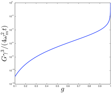
Figure 1: Normalized Fisher information versus $g$ on logarithmic scale for $\Gamma=0.01$.

References

- Irwin and Hilton (2005) K. Irwin and G. Hilton, in Cryogenic Particle Detection, Topics in Applied Physics, Vol. 99, edited by C. Enss (Springer Berlin Heidelberg, 2005) pp. 63–150.
- Sachdev (2011) S. Sachdev, Quantum Phase Transitions (Cambridge University Press, Cambridge, 2011).
- Peres (1984) A. Peres, Phys. Rev. A 30, 1610 (1984).
- Gorin et al. (2006) T. Gorin, T. Prosen, T. H. Seligman, and M. Žnidarič, Phys. Rep. 435, 33 (2006).
- Goussev et al. (2012) A. Goussev, R. A. Jalabert, H. M. Pastawski, and D. Wisniacki, ArXiv e-prints (2012), arXiv:1206.6348 [nlin.CD] .
- Helstrom (1976) C. W. Helstrom, Quantum Detection and Estimation Theory (Academic Press, New York, 1976).
- Walls and Milburn (2008) D. F. Walls and G. J. Milburn, Quantum Optics (Springer-Verlag, Berlin, 2008).
- Dicke (1954) R. H. Dicke, Phys. Rev. 93, 99 (1954).
- Emary and Brandes (2003) C. Emary and T. Brandes, Phys. Rev. E 67, 066203 (2003).
- Quan et al. (2006) H. T. Quan, Z. Song, X. F. Liu, P. Zanardi, and C. P. Sun, Phys. Rev. Lett. 96, 140604 (2006).
- Nielsen and Chuang (2000) M. A. Nielsen and I. L. Chuang, Quantum Computation and Quantum Information (Cambridge University Press, Cambridge, 2000).
- Ou (1996) Z. Y. Ou, Phys. Rev. Lett. 77, 2352 (1996).
- Paris (1997) M. G. Paris, Physics Letters A 225, 23 (1997).
- Childs et al. (2000) A. M. Childs, J. Preskill, and J. Renes, J. Mod. Opt. 47, 155 (2000).
- Acín (2001) A. Acín, Phys. Rev. Lett. 87, 177901 (2001).
- Acín et al. (2001) A. Acín, E. Jané, and G. Vidal, Phys. Rev. A 64, 050302(R) (2001).
- D’Ariano et al. (2001) G. M. D’Ariano, P. Lo Presti, and M. G. A. Paris, Phys. Rev. Lett. 87, 270404 (2001).
- Tsang and Nair (2012) M. Tsang and R. Nair, Phys. Rev. A 86, 042115 (2012).
- Tsang (2013) M. Tsang, New Journal of Physics 15, 073005 (2013).
- Hayashi (2006) M. Hayashi, Quantum Information (Springer, Berlin, 2006).
- Paris (2009) M. G. A. Paris, International Journal of Quantum Information 7, 125 (2009).
- Tsang et al. (2011) M. Tsang, H. M. Wiseman, and C. M. Caves, Phys. Rev. Lett. 106, 090401 (2011).
- Zanardi et al. (2007) P. Zanardi, P. Giorda, and M. Cozzini, Phys. Rev. Lett. 99, 100603 (2007).
- Fujiwara (2006) A. Fujiwara, Journal of Physics A: Mathematical and General 39, 12489 (2006).
- Tsang (2012) M. Tsang, Phys. Rev. Lett. 108, 230401 (2012).
- Giovannetti and Maccone (2012) V. Giovannetti and L. Maccone, Phys. Rev. Lett. 108, 210404 (2012).
- Zanardi et al. (2008) P. Zanardi, M. G. A. Paris, and L. Campos Venuti, Phys. Rev. A 78, 042105 (2008).
- Invernizzi and Paris (2010) C. Invernizzi and M. G. Paris, J. Mod. Opt. 57, 198 (2010).
- Gammelmark and Mølmer (2011) S. Gammelmark and K. Mølmer, New J. Phys. 13, 053035 (2011).
- Cucchietti (2010) F. M. Cucchietti, J. Opt. Soc. Am. B 27, A30 (2010).
- Giovannetti et al. (2004) V. Giovannetti, S. Lloyd, and L. Maccone, Science 306, 1330 (2004).
- Lloyd (2000) S. Lloyd, Phys. Rev. A 62, 022108 (2000).
- Mabuchi and Khaneja (2005) H. Mabuchi and N. Khaneja, International Journal of Robust and Nonlinear Control 15, 647 (2005).
- Wiseman and Milburn (2010) H. M. Wiseman and G. J. Milburn, Quantum Measurement and Control (Cambridge University Press, Cambridge, 2010).
- Cai et al. (2012) C. Y. Cai, Q. Ai, H. T. Quan, and C. P. Sun, Phys. Rev. A 85, 022315 (2012).
- Lambert et al. (2012) N. Lambert, Y.-N. Chen, Y.-C. Cheng, C.-M. Li, G.-Y. Chen, and F. Nori, Nature Physics 9, 10 (2012).
- Silva (2008) A. Silva, Phys. Rev. Lett. 101, 120603 (2008).
- Santiago and Vaidya (1976) M. A. M. Santiago and A. N. Vaidya, J. Phys. A 9, 897 (1976).
- Kennedy (1973) R. S. Kennedy, MIT RLE Quart. Prog. Rep. 108, 219 (1973).
- Gardiner and Zoller (2004) C. W. Gardiner and P. Zoller, Quantum Noise (Springer-Verlag, Berlin, 2004).
- (41) See Supplementary Material for supporting calculations.
- Sato et al. (1998) T. Sato, Y. Kakizawa, and M. Taniguchi, Australian & New Zealand Journal of Statistics 40, 17 (1998).
- Shumway and Stoffer (2006) R. H. Shumway and D. S. Stoffer, Time Series Analysis and Its Applications (Springer, New York, 2006).
- Ang et al. (2013) S. Z. Ang, G. I. Harris, W. P. Bowen, and M. Tsang, ArXiv e-prints (2013), arXiv:1307.3800 [physics.optics] .
- Vahala (2003) K. J. Vahala, Nature 424, 839 (2003).
- Kippenberg and Vahala (2008) T. J. Kippenberg and K. J. Vahala, Science 321, 1172 (2008).
- Safavi-Naeini et al. (2012) A. H. Safavi-Naeini, J. Chan, J. T. Hill, T. P. M. Alegre, A. Krause, and O. Painter, Phys. Rev. Lett. 108, 033602 (2012).
- Kippenberg et al. (2004) T. J. Kippenberg, S. M. Spillane, and K. J. Vahala, Phys. Rev. Lett. 93, 083904 (2004).
- Rokhsari et al. (2005) H. Rokhsari, T. Kippenberg, T. Carmon, and K. Vahala, Opt. Express 13, 5293 (2005).
- Baumann et al. (2010) K. Baumann, C. Guerlin, F. Brennecke, and T. Esslinger, Nature 464, 1301 (2010).
- Paraan and Silva (2009) F. N. C. Paraan and A. Silva, Phys. Rev. E 80, 061130 (2009).
- Fujiwara and Imai (2008) A. Fujiwara and H. Imai, Journal of Physics A: Mathematical and Theoretical 41, 255304 (2008).
- Escher et al. (2011) B. M. Escher, R. L. de Matos Filho, and L. Davidovich, Nature Physics 7, 406 (2011).
- Escher et al. (2011) B. M. Escher, R. L. de Matos Filho, and L. Davidovich, Brazilian Journal of Physics 41, 229 (2011).
- Escher et al. (2012) B. M. Escher, L. Davidovich, N. Zagury, and R. L. de Matos Filho, Phys. Rev. Lett. 109, 190404 (2012).
- Kołodyński and Demkowicz-Dobrzański (2010) J. Kołodyński and R. Demkowicz-Dobrzański, Phys. Rev. A 82, 053804 (2010).
- Demkowicz-Dobrzański et al. (2012) R. Demkowicz-Dobrzański, J. Kołodyński, and M. Guţă, Nature Communications 3, 1063 (2012), arXiv:1201.3940 [quant-ph] .
- Kołodyński and Demkowicz-Dobrzański (2013) J. Kołodyński and R. Demkowicz-Dobrzański, ArXiv e-prints (2013), arXiv:1303.7271 [quant-ph] .
- Knysh et al. (2011) S. Knysh, V. N. Smelyanskiy, and G. A. Durkin, Phys. Rev. A 83, 021804 (2011).
- Bastidas et al. (2012a) V. M. Bastidas, C. Emary, B. Regler, and T. Brandes, Phys. Rev. Lett. 108, 043003 (2012a).
- Bastidas et al. (2012b) V. M. Bastidas, C. Emary, G. Schaller, and T. Brandes, Phys. Rev. A 86, 063627 (2012b).
- Engelhardt et al. (2012) G. Engelhardt, V. M. Bastidas, C. Emary, and T. Brandes, ArXiv e-prints (2012), arXiv:1211.2683 [quant-ph] .
- Van Trees (2001) H. L. Van Trees, Detection, Estimation, and Modulation Theory, Part III: Radar-Sonar Signal Processing and Gaussian Signals in Noise (John Wiley & Sons, New York, 2001).