One-dimensional quantum walks via generating function and the CGMV method

Abstract We treat a quantum walk (QW) on the line whose quantum coin at each vertex tends to be the identity as the distance goes to infinity. We obtain a limit theorem that this QW exhibits localization with not an exponential but a “power-law” decay around the origin and a “strongly” ballistic spreading called bottom localization in this paper. This limit theorem implies the weak convergence with linear scaling whose density has two delta measures at $x=0$ (the origin) and $x=1$ (the bottom) without continuous parts.

1 Introduction

Quantum walks (QWs) are considered as quantum counterparts of random walks [1]. Primitive forms of QWs on lines have already appeared as discrete time and space analogue of a relativistic motion of a free particle known as the Feynman checkerboard [2], and a toy model to construct the quantum probability theory discussed in [3]. The QWs on the line treated in our paper are denoted by a complex-valued sequence $(\gamma_{j})_{j\in\mathbb{Z}}$ ($0\leq|\gamma_{j}|\leq 1$). The square absolute value of each parameter $\gamma_{j}$ assigned at each vertex $j$, $|\gamma_{j}|^{2}$, corresponds to a reflection strength at each vertex. For an extreme case, $|\gamma_{j}|=0$ for all $j$, the walk has no reflection. Thus in this case, the scaled distance from the origin weakly converges as follows:

$$X_{n}/n\Rightarrow\delta_{1}(x)\;\;(n\to\infty),$$

where $\Rightarrow$ means weak convergence. The generating function is one of the effective tools to get stochastic behaviors of QWs with $|\gamma_{j}|<1$, for example, localization and weak convergence [5, 6, 7, 8]. The two functions $g_{j}^{(\pm)}:\mathbb{C}\to\mathbb{C}$ ($j\in\mathbb{Z}$) determined by the following continued fraction relationship give an expression for the generating function [8].

$$\widetilde{g}^{(+)}_{j+1}(z)=-\frac{z^{2}\overline{\gamma}_{j+1}+\widetilde{g}^{(+)}_{j}}{z^{2}+\gamma_{j+1}\widetilde{g}^{(+)}_{j}}\;\;\mathrm{and}\;\;\widetilde{g}^{(-)}_{j-1}(z)=-\frac{-z^{2}\gamma_{j-1}+\widetilde{g}^{(-)}_{j}}{z^{2}-\overline{\gamma}_{j-1}\widetilde{g}^{(-)}_{j}}.$$ (1.1)

Indeed, for spatial homogeneous case, i.e., its coin parameters are $\gamma_{j}=\gamma$, the generating function plays an important role to show that the walks belong to a universality class of QWs [6, 7, 8], that is,

$$X_{n}/n\Rightarrow c\delta_{0}(x)+(1-c)r(x)f_{K}(x;\rho),\;\;(n\to\infty)$$

where $f_{K}(x;\rho)$ has anti-bell shape with the finite support $|x|\in[0,\rho)$ ($\rho=\sqrt{1-|\gamma|^{2}}$), and $c\in[0,1)$ reflects a localization property, and the rational polynomial $r(x)$ depends on the setting of the walk, for example, the initial state [6, 11], boundary condition [7, 9], and spatial one defect [8]. Here, $f_{K}(x;\rho)$ was first introduced by [11, 12] (2002)

$$f_{K}(x;\rho)=\frac{\boldsymbol{1}_{\{|x|<\rho\}}(x)|\gamma|}{\pi(1-x^{2})\sqrt{\rho^{2}-x^{2}}}.$$ (1.2)

It has been a quite interesting problem to get a limit theorem corresponding to the above weak convergences in the case of varied coin parameters in a whole vertices on the line [13, 14, 15]. Recently, it was shown that QWs on the line are described by the CMV matrix [18]. The CMV matrix is a minimal representation of recurrence relations between the orthogonal polynomials of a measure $\mu$ on the unit circle determined by the Schur parameter $(\gamma_{0},\gamma_{1},\dots)$ [16, 17]. There is a nice review on the relationship between QWs and the CMV matrix [4]. A well developed theory of the spectral analysis of the CMV matrix[19] advantages the analysis of QWs, especially, its spectrum. Indeed, for a sequence of homogeneous Schur parameter $\gamma_{j}=\gamma$ ($0<|\gamma|<1$), the spectral measure is described by

$$d\mu(e^{i\theta})=w(e^{i\theta})\frac{d\theta}{2\pi}+\sum_{j}c_{j}\delta(e^{i\theta}-e^{i\theta_{j}}),$$ (1.3)

where $w(e^{i\theta})$ is an absolutely continuous part which has a finite support $\{\theta\in[0,2\pi);|\cos\theta|\leq\rho\}$, and $c_{j}>0$ is a mass at $e^{i\theta_{j}}$. For the extreme cases, $|\gamma|=0$ implies $d\mu$ becomes the uniform measure on $[0,2\pi)$. The existence of the mass point gives localization property of the QW [10]. On the other hand, the absolutely continuous part is related to a ballistic transport, in fact, the real part of the support for the spectral measure, $\rho$, reflects the stochastic property in the weak limit measure of the QW, that is, the walk frequency exists between $|x|\leq\rho n$. The Schur function $f:\mathbb{C}\to\mathbb{C}$ has an important role to describe the spectral measure. The Schur function is obtained by the following continuum fractional expression known as the Schur algorithm:

$$f_{0}(z)=f(z);\;f_{j+1}(z)=\frac{1}{z}\frac{f_{j}(z)-\gamma_{j}}{1-\overline{\gamma_{j}}f_{j}(z)},\;j\geq 0.$$ (1.4)

Comparing Eq. (1.4) with Eq. (1.1), we get a relationship (see Lemma 3) which connects the spectral analysis of the CMV matrix between the generating function of QWs. The QW treated here has position dependent coin parameters which tends to zero as the distance from the origin goes to infinity. More concretely, the coin parameters are $\gamma_{j}=1/(r+j)$ for $j\in\{0,1,\dots\}$ with $r>1$. Our results on the QWs treated here suggest that this relationship can be a key to get detailed stochastic behaviors of QWs from its spectral analysis. On the other hand, Refs. [21] and [22] focus on an inclusive relationship between the recurrence properties proposed by [20, 21] and its spectrum. We obtain an explicit expression for the limit distribution outside the universality class. For our best knowledge, this is the first result on an explicit expression for the limit distribution of a position dependent QW over the whole vertices: we show co-existence of localization with power-law decay around the origin and a strongly ballistic transport. (See Theorems 3 and 4.)

This paper is organized as follows. In Sect. 2, we give the definitions of the QWs on the line and present its generating functions in a general setting. Connections between the CMV matrix and the QWs are devoted in Sect. 3. Using this relationship obtained by Sect. 3, we compute limit theorems concretely for a spatial dependent QW with the coin parameter $\gamma_{j}=1/(r+j)$ in Sect. 4. Finally, we give a summary and discussion in Sect 5.

2 Generating function of quantum walks

From now on, we consider the three types of QWs; (i) first kind of QW on infinite half line (H-QW(1)), (ii) second kind of QW on half infinite line (H-QW(2)), and (iii) QW on doubly infinite line (D-QW). The detailed definitions are in the following:

Definition 1.

We assign two dimensional unitary matrices $\{H_{j}\}_{j\in\mathbb{Z}}$ at each vertex of $\mathbb{Z}$. Put the two Hilbert spaces considering here as $\mathcal{H}_{+}=\mathrm{span}\{\boldsymbol{\delta}_{j,L},\boldsymbol{\delta}_{j,R};j\in\mathbb{Z}_{+}\}$ and $\mathcal{H}=\mathrm{span}\{\boldsymbol{\delta}_{j,L},\boldsymbol{\delta}_{j,R};j\in\mathbb{Z}\}$. The walks start with the initial state $\alpha\boldsymbol{\delta}_{0,L}+\beta\boldsymbol{\delta}_{0,R}$ where $\alpha,\beta\in\mathbb{C}$ with $|\alpha|^{2}+|\beta|^{2}=1$.

1. First kind of QW on half line (H-QW(1))
   Total state space: $\mathcal{H}_{+}$
   Time evolution $E=SC$ on $\mathcal{H}_{+}$:

   $$C =\bigoplus_{j\in\mathbb{Z}_{+}}H_{j},$$ (2.5)

   $$S\boldsymbol{\delta}_{j,L} =\begin{cases}\boldsymbol{\delta}_{j-1,L}&\text{: $j\geq 1$}\\ \boldsymbol{\delta}_{0,R}&\text{: $j=0$ }\end{cases},\;S\boldsymbol{\delta}_{j,R}=\boldsymbol{\delta}_{j+1,R}.$$ (2.6)

2. Second kind of QW on half line (H-QW(2))
   Total state space: $\mathcal{H}_{+}$
   Time evolution $E=SC$ on $\mathcal{H}_{+}$: We choose quantum coin at the origin and the initial coin state so that $\langle\boldsymbol{\delta}_{0,R},H_{0}\boldsymbol{\delta}_{0,R}\rangle=\langle\boldsymbol{\delta}_{0,L},H_{0}\boldsymbol{\delta}_{0,L}\rangle=0$, and $\beta=0$. Then

   $$C =\bigoplus_{j\in\mathbb{Z}_{+}}H_{j}\mathrm{\;with\;}(H_{0})_{\boldsymbol{\delta}_{0,J},\boldsymbol{\delta}_{0,J}}=0\mathrm{\;for\;}J\in\{L,R\}.$$ (2.7)

   $$S\boldsymbol{\delta}_{j,L} =\boldsymbol{\delta}_{j-1,L},\;S\boldsymbol{\delta}_{j,R}=\boldsymbol{\delta}_{j+1,R}.$$ (2.8)

3. QW on doubly infinite line (D-QW)
   Total state space: $\mathcal{H}$
   Time evolution $E=SC$ on $\mathcal{H}$:

   $$C =\bigoplus_{j\in\mathbb{Z}_{+}}H_{j}$$ (2.9)

   $$S\boldsymbol{\delta}_{j,L} =\boldsymbol{\delta}_{j-1,L},\;S\boldsymbol{\delta}_{j,R}=\boldsymbol{\delta}_{j+1,R}.$$ (2.10)

We should remark that the subspace of $\mathcal{H}_{+}$, $\mathrm{span}\{\{\boldsymbol{\delta}_{0,L}\}\cup\{\boldsymbol{\delta}_{j,L},\boldsymbol{\delta}_{j,R};j\geq 1\}\}$, is invariant under the action of the time evolution of H-QW(2). Put $\langle\boldsymbol{\delta}_{j,L},H_{j}\boldsymbol{\delta}_{j,L}\rangle=a_{j}$, $\langle\boldsymbol{\delta}_{j,L},H_{j}\boldsymbol{\delta}_{j,R}\rangle=b_{j}$, $\langle\boldsymbol{\delta}_{j,R},H_{j}\boldsymbol{\delta}_{j,L}\rangle=c_{j}$, $\langle\boldsymbol{\delta}_{j,R},H_{j}\boldsymbol{\delta}_{j,R}\rangle=d_{j}$. The matrix representations for the time evolutions of H-QW(1), H-QW(2) and D-QW are expressed by $E_{1}$, $E_{2}$, and $E_{D}$, respectively as follows:

$$E_{1}=\left[\begin{array}[]{cc|cc|cc|cc|c}0&0&a_{1}&b_{1}&&&&&\\ a_{0}&b_{0}&0&0&&&&&\\ \hline\cr 0&0&&&a_{2}&b_{2}&&&\\ c_{0}&d_{0}&&&0&0&&&\\ \hline\cr&&0&0&&&a_{3}&b_{3}&\\ &&c_{1}&d_{1}&&&0&0&\\ \hline\cr&&&&0&0&&&\ddots\\ &&&&c_{2}&d_{2}&&&\\ \hline\cr&&&&&&\ddots&&\ddots\end{array}\right],\;\;E_{2}=\left[\begin{array}[]{c|cc|cc|cc|c}0&a_{1}&b_{1}&&&&&\\ \hline\cr 0&&&a_{2}&b_{2}&&&\\ c_{0}&&&0&0&&&\\ \hline\cr&0&0&&&a_{3}&b_{3}&\\ &c_{1}&d_{1}&&&0&0&\\ \hline\cr&&&0&0&&&\ddots\\ &&&c_{2}&d_{2}&&&\\ \hline\cr&&&&&\ddots&&\ddots\end{array}\right]$$

$$E_{D}=\left[\begin{array}[]{c|cc|cc|cc|cc|c}\ddots&&\ddots&&&&&&&\\ \hline\cr&&&a_{-1}&b_{-1}&&&&&\\ \ddots&&&0&0&&&&&\\ \hline\cr&0&0&&&a_{0}&b_{0}&&&\\ &c_{-2}&d_{-2}&&&0&0&&&\\ \hline\cr&&&0&0&&&a_{1}&b_{1}&\\ &&&c_{-1}&d_{-1}&&&0&0&\\ \hline\cr&&&&&0&0&&&\ddots\\ &&&&&c_{0}&d_{0}&&&\\ \hline\cr&&&&&&&\ddots&&\ddots\end{array}\right],$$

where the orders of the basis in the above matrices for H-QW(1), H-QW(2) and D-QW are

$$((0,L),(0,R),(1,L),(1,R),(2,L),(2,R),\dots),\;((0,L),(1,L),(1,R),(2,L),(2,R),\dots)$$

$$\mathrm{and}$$

$$(\dots,(-1,L),(-1,R),(0,L),(0,R),(1,L),(1,R),\dots),$$

respectively. The following lemma obtained by [4, 10] is useful to simplify our model.

Lemma 1.

Put the quantum coin assigned at position $j$ described by complex valued parameter $\gamma_{j}$ with $|\gamma_{j}|<1$ as

$$H_{j}^{(\gamma_{j})}=\begin{bmatrix}\rho_{j}&\overline{\gamma}_{j}\\ -\gamma_{j}&\rho_{j}\end{bmatrix}$$ (2.11)

where $\rho_{j}=\sqrt{1-|\gamma_{j}|^{2}}$, and we put $\boldsymbol{\delta}_{j,L}\cong{}^{T}[1,0]$, $\boldsymbol{\delta}_{j,R}\cong{}^{T}[0,1]$ on the subspace of $\mathcal{H}_{j}\equiv\mathrm{span}\{\boldsymbol{\delta}_{j,L},\boldsymbol{\delta}_{j,R}\}$. Then for each case of QW, i.e., H-QW(1), H-QW(2) and D-QW, with quantum coins $\{H_{j}\}_{j}$, there exists an infinite diagonal matrix $D$ on $\mathcal{H}$ and a sequence of complex-valued parameters $\boldsymbol{\gamma}\equiv(\gamma_{j})_{j}$ with $|\gamma_{j}|<1$, such that

$$E=D^{\dagger}U^{(\boldsymbol{\gamma})}D.$$ (2.12)

Here $U^{(\boldsymbol{\gamma})}=SC^{(\boldsymbol{\gamma})}$, where $C^{(\boldsymbol{\gamma})}=\bigoplus_{j}H_{j}^{(\gamma_{j})}$.

So we get a one-to-one correspondence between each QW and pair of the diagonal matrix $D$ and the parameters $(\gamma_{j})_{j}$. From now on, we concentrate on the walks with the time evolution $U^{(\boldsymbol{\gamma})}$ for simplicity. We call $(\gamma_{j})_{j}$ coin parameter.

Let $\Xi_{n}:\mathbb{Z}\to M_{2}(\mathbb{C})$ be defined by

$$\Xi_{n}(j)\equiv\begin{bmatrix}\langle\boldsymbol{\delta}_{j,L},{U^{(\boldsymbol{\gamma)}}}^{n}\boldsymbol{\delta}_{0,L}\rangle&\langle\boldsymbol{\delta}_{j,L},{U^{(\boldsymbol{\gamma)}}}^{n}\boldsymbol{\delta}_{0,R}\rangle\\ \langle\boldsymbol{\delta}_{j,R},{U^{(\boldsymbol{\gamma)}}}^{n}\boldsymbol{\delta}_{0,L}\rangle&\langle\boldsymbol{\delta}_{j,R},{U^{(\boldsymbol{\gamma)}}}^{n}\boldsymbol{\delta}_{0,L}\rangle\end{bmatrix}$$ (2.13)

We put $\Xi_{n}(j)=0$ for negative $j$ in the cases of H-QW(1) and (2). Define

$$P_{j}=\begin{bmatrix}\rho_{j}&\overline{\gamma}_{j}\\ 0&0\end{bmatrix},\;Q_{j}=\begin{bmatrix}0&0\\ -\gamma_{j}&\rho_{j}\end{bmatrix},\;R_{j}=\begin{bmatrix}-\gamma_{j}&\rho_{j}\\ 0&0\end{bmatrix},\;S_{j}=\begin{bmatrix}0&0\\ \rho_{j}&\overline{\gamma}_{j}\end{bmatrix}.$$ (2.14)

We call $\Xi_{n}$ weight of passages with length $n$ in the following sense: from a simple observation, we obtain the following recursion equations : for H-QW(II) and D-QW,

$$\Xi_{n}(j)=P_{j+1}\Xi_{n-1}(j+1)+Q_{j-1}\Xi_{n-1}(j-1),$$ (2.15)

and for H-QW(I)

$$\Xi_{n}(j)=\begin{cases}P_{j+1}\Xi_{n-1}(j+1)+Q_{j-1}\Xi_{n-1}(j-1)&\text{$j\geq 1$,}\\ P_{1}\Xi_{n-1}(j+1)+S_{0}\Xi_{n-1}(0)&\text{$j=0$.}\end{cases}$$ (2.16)

For $z\in\mathbb{C}$ with $|z|\leq 1$, we denote a generating function with respect to time $n$ as $\widetilde{\Xi}_{j}(z)\equiv\sum_{n\geq 0}\Xi_{n}(j)z^{n}$. Here to express the generating function, we define $\widetilde{g}^{(\pm)}_{j}(z)$ in the following continued-fraction representation: for $j\in\mathbb{Z}$,

$$\widetilde{g}^{(+)}_{j}(z) =\begin{cases}-\frac{z^{2}}{\gamma_{j+1}}\left(1-\frac{\rho_{j+1}^{2}}{1+\gamma_{j+1}\widetilde{g}^{(+)}_{j+1}(z)}\right),&\text{: $\gamma_{j+1}\neq 0$}\\ z^{2}\widetilde{g}^{(+)}_{j+1}&\text{: $\gamma_{j+1}=0$}\end{cases}$$ (2.17)

$$\widetilde{g}^{(-)}_{j}(z) =\begin{cases}-\frac{z^{2}}{\overline{\gamma}_{j-1}}\left(1-\frac{\rho_{j-1}^{2}}{1-\overline{\gamma}_{j-1}\widetilde{g}^{(-)}_{j-1}(z)}\right),&\text{: $\gamma_{j-1}\neq 0$, }\\ z^{2}\widetilde{g}^{(-)}_{j-1}(z),&\text{: $\gamma_{j-1}=0.$}\end{cases}$$ (2.18)

We call $\widetilde{g}^{(+)}_{j}(z)$ (resp. $\widetilde{g}^{(-)}_{j}(z)$) “positive (resp. negative) $j$-th g-function” , respectively. We should note that for $j\geq 0$, $\widetilde{g}^{(+)}_{j}(z)$ only depends on at most parameters $(\gamma_{1},\gamma_{2},\dots)$ and also $\widetilde{g}^{(+)}_{j}(z)$ only depends on at most parameters $(\gamma_{-1},\gamma_{-2},\dots)$. To emphasize its dependences, we sometimes denote $\widetilde{g}^{(+)}_{j}(z)\equiv\widetilde{g}_{j}^{(+),\;(\gamma_{1},\gamma_{2},\dots)}(z)$ for $j\geq 0$, and $\widetilde{g}^{(-)}_{j}(z)\equiv\widetilde{g}_{j}^{(-),\;(\gamma_{-1},\gamma_{-2},\dots)}(z)$ for $j\leq 0$.

Denote $F^{(+)}_{n}(j)$ (resp. $F^{(-)}_{n}(j)$) as the weight of all passages which start from $j$ and return to the same position $j$ at time $n$ avoiding $\{i\in\mathbb{Z}:i<j\}$ (resp. $\{i\in\mathbb{Z}:i>j\}$) throughout the time interval $0<s<n$, respectively. Indeed, the generating function $\widetilde{F}^{(\pm)}_{j}(z)\equiv\sum_{n\geq 1}F^{(\pm)}_{j}(n)z^{n}$ can be expressed by using $\widetilde{g}^{(+)}_{j}(z)$ and $\widetilde{g}^{(-)}_{j}(z)$ as follows:

$$\widetilde{F}^{(+)}_{j}(z) =\begin{cases}\widetilde{g}^{(+)}_{j}(z)R_{j}&\text{: H-QW(2) and D-QW,}\\ \widetilde{g}^{(+)}_{j}(z)R_{j}+z\delta_{0}(j)S_{0}&\text{: H-QW(1), }\end{cases}$$ (2.19)

$$\widetilde{F}^{(-)}_{j}(z) =\widetilde{g}^{(-)}_{j}(z)S_{j}.$$ (2.20)

Then we give an expression for the generating function using $\{\widetilde{g}^{(+)}_{j}(z)\}_{j\in\mathbb{N}}$ and $\{\widetilde{g}^{(-)}_{j}(z)\}_{j\in\mathbb{N}}$ in the following lemma. We put $\rho_{-1}=0$ for H-QW(1) and H-QW(2) cases.

Lemma 2.

1. If $j=0$, then

   $$\widetilde{\Xi}_{0}(z)=\begin{cases}\frac{1}{1-\overline{\gamma}_{0}z+(\gamma_{0}-z)\widetilde{g}^{(+)}_{0}(z)}\begin{bmatrix}1-\overline{\gamma}_{0}z&\rho_{0}\widetilde{g}^{(+)}_{0}(z)\\ \rho_{0}z&1+\gamma_{0}\widetilde{g}^{(+)}_{0}(z)\end{bmatrix},&\text{: H-QW(1), }\\ \frac{1}{1-\widetilde{g}^{(+)}_{0}(z)}\begin{bmatrix}1&0\\ 0&1-\widetilde{g}^{(+)}_{0}(z)\end{bmatrix},&\text{: H-QW(2),}\\ \frac{1}{1+\gamma_{0}\widetilde{g}^{(+)}_{0}(z)-\overline{\gamma}_{0}\widetilde{g}^{(-)}_{0}(z)-\widetilde{g}^{(+)}_{0}(z)\widetilde{g}^{(-)}_{0}(z)}\begin{bmatrix}1-\overline{\gamma}_{0}\widetilde{g}^{(-)}_{0}(z)&\rho_{0}\widetilde{g}^{(+)}_{0}(z)\\ \rho_{0}\widetilde{g}^{(-)}_{0}(z)&1+\gamma_{0}\widetilde{g}^{(+)}_{0}(z)\end{bmatrix},&\text{: D-QW}\end{cases}$$ (2.21)

2. if $|j|\geq 1$, then

   $$\\ \widetilde{\Xi}_{j}(z)=\begin{cases}\left\{\delta_{1}(j)+(1-\delta_{1}(j))\widetilde{\lambda}^{(+)}_{j-1}(z)\cdots\widetilde{\lambda}^{(+)}_{1}(z)\right\}\begin{bmatrix}\widetilde{\lambda}^{(+)}_{j}(z)\widetilde{g}^{(+)}_{j}(z)\\ z\end{bmatrix}\begin{bmatrix}-\gamma_{0}&\rho_{0}\end{bmatrix}\widetilde{\Xi}_{0}(z)&\text{: $j\geq 1$, }\\ \\ \left\{\delta_{-1}(j)+(1-\delta_{-1}(j))\widetilde{\lambda}^{(-)}_{j+1}(z)\cdots\widetilde{\lambda}^{(-)}_{1}(z)\right\}\begin{bmatrix}z\\ \widetilde{\lambda}^{(-)}_{j}(z)\widetilde{g}^{(-)}_{j}(z)\end{bmatrix}\begin{bmatrix}\rho_{0}&\overline{\gamma}_{0}\end{bmatrix}\widetilde{\Xi}_{0}(z)&\text{: $j\leq-1$, }\end{cases}$$ (2.22)

where $\widetilde{\lambda}^{(+)}_{j}(z)=z\rho_{j}/(1+\gamma_{j}\widetilde{g}^{(+)}_{j}(z))$, $\widetilde{\lambda}^{(-)}_{j}(z)=z\rho_{j}/(1-\overline{\gamma}_{j}\widetilde{g}^{(-)}_{j}(z))$.

Proof.

As consequences of the D-QW case, we obtain the H-QWs (1) and (2) cases as follows: We omit the proof of the D-QW because we can see the detailed proof in [8].

1. H-QW(1) case: Put $\widetilde{\Xi}_{j,D}(z)$ as the generating function at position $j$ whose coin parameters are $\gamma_{2j}=\alpha_{j}$, $\gamma_{2j-1}=0$, $(j\neq 0)$, $=-1$, $(j=0)$ for $j\in\mathbb{Z}$. We put its g-functions as $\{\widetilde{g}_{j,D}^{(+)}(z)\}_{j}$ and $\{\widetilde{g}_{j,D}^{(-)}(z)\}_{j}$. On the other hand, $\widetilde{\Xi}_{j,H(1)}(z)$ as the generating function at position $j$ whose coin parameters are $\gamma_{j}=\alpha_{j}$ for $j\in\mathbb{Z}_{+}$. We put its g-functions as $\{\widetilde{g}_{j,H(1)}^{(+)}(z)\}_{j}$ and $\{\widetilde{g}_{j,H(1)}^{(-)}(z)\}_{j}$. From the definition of H-QW(1), we have

   $$\widetilde{\Xi}_{j,H(1)}(z^{2})=\widetilde{\Xi}_{2j,D}(z),\;\;(j\in\mathbb{Z}_{+})$$ (2.23)

   Note that

   $$\widetilde{g}_{2j,D}^{(+)}(z)=-\frac{z^{4}}{\alpha_{j+1}}\left(1-\frac{|\rho_{j+1}|^{2}}{1+\alpha_{j+1}\widetilde{g}_{2j+2,D}^{(+)}(z)}\right),$$ (2.24)

   which implies $\widetilde{g}_{2j,D}^{(+)}(z)=\widetilde{g}_{j,H(1)}^{(+)}(z^{2})$. Also note that $\widetilde{g}_{0,D}^{(-)}(z)=z^{2}$. Therefore substituting the above expressions of $\widetilde{g}_{0,D}^{(\pm)}(z)$ into Eq. (2.21) for D-QW case and Eq. (2.22), we have the generating function for $\gamma_{2j}=\alpha_{j}$, $\gamma_{2j-1}=0$, $(j\neq 0)$, $=-1$, $(j=0)$ ($j\in\mathbb{Z}$) case. Then from Eq. (2.23), we obtain Eq. (2.21) for H-QW(1) case.

2. H-QW(2) case: The definition of the H-QW(2) yields that replacing $\widetilde{g}^{(-)}_{0}(z)=0$ and $\gamma_{0}=-1$ for D-QW case in EQ. (2.21) gives the generating function for H-QW(2) in Eq. (2.21).

∎

Combining Lemma 2 with the spatial Fourier analysis, we obtain the following weak limit theorems for H-QW(1)[9], H-QW(2)[7], and D-QW [11] with homogeneous coin parameter $\gamma_{j}=\gamma\in\mathbb{C}$ with $0<|\gamma|<1$.

Theorem 1 ([7],[9],[11]).

The walks with coin parameter $\alpha_{j}=\gamma$ start at the origin with the initial coin states ${}^{T}[\alpha,\beta]$ (for H-QW(1), and D-QW), and ${}^{T}[1,0]$ (H-QW(2)), respectively. Then we have

$$\frac{X_{n}}{n}\Rightarrow c\delta_{0}(x)+w(x)f_{K}(x;\rho)\;\;(n\to\infty),$$ (2.25)

where

$$c= \begin{cases}\frac{\mathrm{Re}^{2}(\gamma)}{1-\mathrm{Im}^{2}(\gamma)}\left|\alpha+\beta\nu(\gamma)\right|^{2}\frac{1+\nu^{2}(\gamma)}{1-\nu^{2}(\gamma)}&\text{: H-QW(1)}\\ \\ \boldsymbol{1}_{\{|\gamma|^{2}+\mathrm{Re}(\gamma)>0\}}(\gamma)\frac{2(|\gamma|^{2}+\mathrm{Re}(\gamma))}{|1+\gamma|^{2}}&\text{: H-QW(2)}\\ \\ 0&\text{: D-QW}\end{cases}$$ (2.26)

$$w(x)= \begin{cases}\boldsymbol{1}_{\{x\geq 0\}}(x)\frac{2|\gamma|^{3}/\rho^{2}\cdot\left\{|\alpha|^{2}+|-\gamma\alpha+\rho\beta|^{2}+2\rho\mathrm{Im}(\gamma)\mathrm{Im}(-\gamma\alpha+\rho\beta)\right\}x^{2}}{\mathrm{Re}^{2}(\gamma)+\mathrm{Im}^{2}(\gamma)x^{2}}&\text{: H-QW(1)}\\ \\ \boldsymbol{1}_{\{x\geq 0\}}(x)\frac{2|\gamma|^{2}(1+\mathrm{Re}(\gamma))x^{2}}{\left(|\gamma|^{2}+\mathrm{Re}(\gamma)\right)^{2}+\mathrm{Im}^{2}(\gamma)x^{2}}&\text{: H-QW(2)}\\ \\ 1-\left(|\alpha|^{2}-|\beta|^{2}+2\mathrm{Re}(\gamma\alpha\overline{\beta})/\rho\right)x&\text{: D-QW}\end{cases}$$ (2.27)

Here $\rho=\sqrt{1-|\gamma|^{2}}$, and $\nu(\gamma)=\mathrm{sgn}(\mathrm{Re}(\gamma))/\rho\cdot\left\{\sqrt{1-\mathrm{Im}^{2}(\gamma)}-|\mathrm{Re}(\gamma)|\right\}$.

The RHS of the first term in Eq. (2.25) provides localization (see Theorem. 2), and the second term provides the ballistic transport. The shape of the weight function $w(x)$ in Eq. (2.27) depends on the boundary condition and initial state. On the other hand, we see $f_{K}(s;\rho)$ commonly for each case. In these cases, the $f_{K}(x;\rho)$ defined in Eq. (1.2) appears as the Jacobian for the change of the variables $x=\partial\theta(k)/\partial k$, i.e.,

$$f_{K}(x;\rho)=\frac{1}{\pi\frac{\partial^{2}\theta(k)}{\partial k^{2}}}\bigg{|}_{x=\partial\theta(k)/\partial k},$$ (2.28)

where $\theta(k)$ is the argument of the singular point for the Fourier transform of the generating function. See Refs. [8, 9], for example, for more detailed computations aroud here.

3 Relation between spectral analysis of CMV matrix and generating function

Let $L^{2}_{\mu}$ be the Hilbert space of $\mu$-square integrable functions whose inner product is

$$(f,g)_{\mu}=\int_{|z|=1}\overline{f(z)}g(z)d\mu,\;f,g\in L^{2}_{\mu}.$$

Let $U$ be a unitary time evolution on $\mathcal{H}$. We consider a complete orthogonal basis system of $L^{2}_{\mu}$ from the order-set $\{1,z^{-1},z,z^{-2},z^{2},\dots\}$. Put $\{\chi_{j}\}_{j}$ as the orthogonal basis system. Then $\chi_{0}(z)=1$,

$$\chi_{2j-1}(z) \in\mathrm{span}\{1,z^{-1},z^{1},\dots,z^{-j}\},$$ (3.29)

$$\chi_{2j}(z) \in\mathrm{span}\{1,z^{-1},z^{1},\dots,z^{-j},z^{j}\}.$$ (3.30)

Thus we obtain the following integral representation:

$$(\chi_{m},z^{n}\chi_{l})_{\mu}=\int_{|z|=1}z^{n}\overline{\chi_{m}(z)}\chi_{l}(z)d\mu(z)$$

In general, there exists a complex-valued sequence called Schur parameter $(\gamma_{0},\gamma_{1},\dots)$ with $|\gamma_{j}|<1$ which denotes five recursion relation between $\{\chi_{m}\}_{m}$, that is, $(\mathcal{C})_{l,m}=(\chi_{l},z\chi_{m})_{\mu}$:

$$\mathcal{C}=\begin{bmatrix}\overline{\gamma}_{0}&\rho_{0}\overline{\gamma}_{1}&\rho_{0}\rho_{1}&0&0&0&0&0&\ldots\\ \rho_{0}&-\gamma_{0}\overline{a}_{1}&-\gamma_{0}\rho_{1}&0&0&0&0&0&\ldots\\ 0&\rho_{1}\overline{\gamma}_{2}&-a_{1}\overline{\gamma}_{2}&\rho_{2}\overline{\gamma}_{3}&\rho_{2}\rho_{3}&0&0&0&\ldots\\ 0&\rho_{1}\rho_{2}&-\gamma_{1}\rho_{2}&-\gamma_{2}\overline{\gamma}_{3}&-\gamma_{2}\rho_{3}&0&0&0&\ldots\\ 0&0&0&\rho_{3}\overline{\gamma}_{4}&-\gamma_{3}\overline{\gamma}_{4}&\rho_{4}\overline{\gamma}_{5}&\rho_{4}\rho_{5}&0&\ldots\\ 0&0&0&\rho_{3}\rho_{4}&-\gamma_{3}\rho_{4}&-\gamma_{4}\overline{\gamma}_{5}&-\gamma_{4}\rho_{5}&0&\ldots\\ &\vdots&\vdots&\vdots&\vdots&\vdots&\ddots&&\end{bmatrix},$$

where $\rho_{j}=\sqrt{1-|\gamma_{j}|^{2}}$. $\mathcal{C}$ is called the CMV matrix. Conversely, if we get $(\gamma_{0},\gamma_{1},\dots)$, the measure on the unit circle is uniquely determined. In fact, the following procedure is a standard method to get the measure from the Schur parameter. Let $f(z)$ be the Schur function with the Schur parameter $(\gamma_{0},\gamma_{1},\dots)$. The Schur function is obtained by the following continuum fractional expression known as Schur algorithm:

$$f_{0}(z)=f(z);\;f_{j+1}(z)=\frac{1}{z}\frac{f_{j}(z)-\gamma_{j}}{1-\overline{\gamma_{j}}f_{j}(z)},\;j\geq 0.$$ (3.31)

To emphasize the dependence of $\gamma_{j}$’s, we express $f_{j}$ as $f_{j}^{(\gamma_{0},\gamma_{1},\dots)}$. The Caratheodory function of the Schur parameter $(\gamma_{0},\gamma_{1},\cdots)$ are defined by

$$F(z)=\frac{1+zf(z)}{1-zf(z)}.$$ (3.32)

An equivalent expression for $F(z)$ is

$$F(z)=\int_{|z|=1}\frac{t+z}{t-z}d\mu(t).$$

The measure $d\mu$ is decomposed into $d\mu(e^{i\theta})=w(e^{i\theta})\frac{d\theta}{2\pi}+d\mu_{s}(e^{i\theta})$, where $w(e^{i\theta})$ is absolutely continuous part called weight, and $\mu_{s}$ is singular part. The weight can be obtained by

$$w(e^{i\theta})=\lim_{r\uparrow 1}\mathrm{Re}(F(re^{i\theta}))$$ (3.33)

The singular points are concentrated on $\{e^{i\theta}:\lim_{r\uparrow 1}\mathrm{Re}(F(r(e^{i\theta})))=\infty\}$, moreover the mass points are given by

$$\mu(\{e^{i\theta}\})=\lim_{r\uparrow 1}\frac{1-r}{2}F(re^{i\theta}).$$ (3.34)

Now we present an expression of the CMV matrix by using second kind of QW. Let $\mathcal{H}_{e}\equiv\mathrm{span}\{\{\boldsymbol{\delta}_{0,L}\}\cup\{\boldsymbol{\delta}_{2j,R},\boldsymbol{\delta}_{2j,L};j\geq 1\}\}\subset\mathcal{H}_{+}$, $\mathcal{H}_{o}\equiv\mathrm{span}\{\boldsymbol{\delta}_{2j+1,R},\boldsymbol{\delta}_{2j+1,L};j\geq 0\}\subset\mathcal{H}_{+}$. Then we obtain a relation between QW and the CMV matrix:

Proposition 1.

Let $U$ be the time evolution of second kind of QW on half line.

$$\mathcal{C}\cong U^{2}|_{\mathcal{H}_{e}},\;{}^{T}\mathcal{C}\cong U^{2}|_{\mathcal{H}_{o}}.$$ (3.35)

Proof.

The CMV matrix $\mathcal{C}$ is decomposed into $\mathcal{C}=\mathcal{L}\mathcal{M}$, where

$$\mathcal{L}=\mathrm{diag}(\Theta_{0},\Theta_{2},\Theta_{4},\dots),\;\mathcal{M}=\mathrm{diag}(1,\Theta_{3},\Theta_{5},\dots),\;\;\mathrm{with}\;\;\Theta_{j}=\begin{bmatrix}\overline{\gamma}_{j}&\rho_{j}\\ \rho_{j}&-{\gamma}_{j}\end{bmatrix}.$$ (3.36)

We interpret $\mathcal{M}$ as $\mathcal{M}:\mathcal{H}_{e}\to\mathcal{H}_{o}$ by relabeling raws and columns of $\mathcal{M}$ as
$(1,R),(1,L),(3,R),(3,L),\dots$ and $(0,L),(2,R),(2,L),(4,R),\dots$, respectively. A simple observation gives $\mathcal{M}=U|_{\mathcal{H}_{e}}$. Conversely, relabeling raws and columns of $\mathcal{L}$ as
$(0,L),(2,R),(2,L),(4,R),\dots$ as $(1,R),(1,L),(3,R),(3,L),\dots$, respectively, we obtain $\mathcal{L}=U|_{\mathcal{H}_{o}}$. So we complete the proof. ∎

The existence of mass points, i.e., “eigenvalues” in the spectrum of the corresponding CMV matrix ensures the localization of QWs. In fact, the limit measure of the localization is obtained by the orthogonal projection onto the eigenspaces of the initial state. We give the following theorem with respect to localization for a space homogeneous case whose parameters are $\gamma_{j}=\gamma$.

Theorem 2 ([10]).

The walks start at the origin with the initial coin state ${}^{T}[\alpha,\beta]$ (for H-QW(1)) and ${}^{T}[1,0]$ (for H-QW(2)), respectively.

$$\lim_{t\to\infty}P(X_{t}^{(I)}=j)=\frac{|\mathrm{Re}(\gamma)|^{2}}{1-\mathrm{Im}(\gamma)^{2}}|\alpha+\beta\nu_{I}(\gamma)|^{2}(1+\nu_{I}^{2}(\gamma))\nu_{I}^{2j}(\gamma),$$

$$P(X^{(II)}_{t}=j)\sim\boldsymbol{1}_{\{|\gamma|^{2}+\mathrm{Re}(\gamma)>0\}}(\gamma)\frac{1+(-1)^{n+j}}{2}\left(\frac{|\gamma|^{2}+\mathrm{Re}(\gamma)}{(1+\gamma)^{2}}\right)^{2}\left(1+\frac{\boldsymbol{1}_{\{j\geq 1\}}(j)}{\nu_{II}^{2}(\gamma)}\right)\nu_{II}^{2j}(\gamma),$$

where

$$\nu_{I}(\gamma)=\frac{\mathrm{sgn}(\mathrm{Re}(\gamma))}{\rho}\left\{\sqrt{1-\mathrm{Im}(\gamma)^{2}}-|\mathrm{Re}(\gamma)|\right\}\;\mathrm{and}\;\nu_{II}(\gamma)=\frac{\rho}{|1+\gamma|}.$$

We should remark that the summation over the positions is strictly smaller than one. The missing value is characterized by Theorem. 1.

In the following, we propose a useful connection between spectral analysis of the CMV matrix and generating function of QWs. The derivation of the above lemma is due to just a simple comparing between Eqs. (2.17) and (3.31).

Lemma 3.

$$\widetilde{g}_{j}^{(+),\;(\gamma_{1},\gamma_{2},\dots)}(z) =z^{2}{f}_{j}^{(\overline{\gamma}_{1},\overline{\gamma}_{2},\dots)}(z^{2}) j\geq 0$$ : , (3.37)

$$\widetilde{g}_{j}^{(-),\;(\gamma_{-1},\gamma_{-2},\dots)}(z) =z^{2}{f}_{|j|}^{(-\gamma_{-1},-\gamma_{-2},\dots)}(z^{2}) j\leq 0$$ : , (3.38)

In the next section, we show an example that the connection works well to get a stochastic behaviors of a QW whose quantum coin at each vertex tends to be transparent as the distance goes to infinity.

4 Stochastic behaviors of spatial dependent quantum walks

Now in this section, we consider H-QW(I) with coin parameter

$$\gamma_{j}=1/(r+j)\;\;(r>1).$$ (4.39)

For each time $n\in\mathbb{N}$, define a map $\mu_{n}:\mathbb{Z}_{+}\to[0,1]$ as

$$\mu_{n}(j)=||\Pi_{j}U^{(\boldsymbol{\gamma})}(\alpha\boldsymbol{\delta}_{0,L}+\beta\boldsymbol{\delta}_{0,R})||^{2}=||\Xi_{n}(j)\varphi_{0}||^{2},$$

where $\Pi_{j}$ is orthogonal projection onto subspace spanned by $\boldsymbol{\delta}_{j,L}$ and $\boldsymbol{\delta}_{j,R}$, and $\varphi_{0}={}^{T}[\alpha,\beta]$. From the unitarity of the time evolution, $\sum_{j\geq 0}\mu_{n}(j)=1$. So we call $\mu_{n}$ distribution of QW at time $n$. We also define a dual distribution of $\mu_{n}$ as $\widetilde{\mu}_{n}(j)\equiv{\mu}_{n}(n-j)$. In this section, our interest focuses on the sequence of distributions $(\mu_{n})_{n\in\mathbb{N}}$ and $(\widetilde{\mu}_{n})_{n\in\mathbb{N}}$. Put for each time $n$, a random variable $X_{n}$ following $\mu_{n}$, that is, $P(X_{n}=j)=\mu_{n}(j)$. To get its generating function, first of all, we consider its spectrum as follows. The Schur function for the Schur parameter $(\gamma_{0},\gamma_{1},\dots)$ is known as (see for example [4])

$$f_{j}(z)=\frac{1}{r+j-(r-1+j)z},\;\;j\in\{0,1,2,\dots\}.$$ (4.40)

On the other hand, combining Lemma 3 with Eq. (4.40) implies

$$\widetilde{g}_{j}^{(+),(\gamma_{1},\gamma_{2},\dots)}(z)=\frac{z^{2}}{r+1+j-(r+j)z^{2}}.$$ (4.41)

Equations (3.32) and (4.40) imply

$$F(z)=\frac{(z+1)(z-r/(r-1))}{(z-1)(z+r/(r-1))}.$$ (4.42)

Then from Eqs. (3.33), (3.34) and (4.42), the spectral measure is

$$d\nu(e^{i\theta})=\frac{\cos^{2}\frac{\theta}{2}}{\cos^{2}\frac{\theta}{2}+\frac{1}{4r(r-1)}}\frac{d\theta}{2\pi}+\frac{1}{2r-1}\delta(e^{i\theta}-1).$$ (4.43)

Note that the coin parameter $\gamma=0$ means that its quantum coin is the identity, that is, perfect transmission. In our model, since $\gamma_{j}\to 0$ $(j\to\infty)$, quantum coin assigned at each vertex tends to the identity as the distance from the origin increases. The full unit circle $\theta\in[0,2\pi)$ of the support for absolutely continuous part of RHS in Eq. (4.43) reflects its argument, since the support of the measure for the QW with coin parameter $(0,0,\dots)$ is also on the full unit circle $\theta\in[0,2\pi)$. Therefore, at the first glance, it seems that the walker gets farther and farther away from the origin. Nevertheless, the measure has also mass point at $\theta=0$. This fact predicts the opposite property, that is, “localization” at the origin as we have already seen other QW models, for example [4, 10]. So what happens to this walk? The following theorem gives its answer.

Theorem 3.

Assume that H-QW(1) whose coin parameter is $(\gamma_{0},\gamma_{1},\dots)$ with $\gamma_{j}=1/(r+j)$ $(r>1)$ is located at the origin with the initial coin state $\varphi_{0}={}^{T}[\alpha,\beta]$ $(|\alpha|^{2}+|\beta|^{2}=1)$. Then we have

1. (Localization around the origin)

   $$\lim_{n\to\infty}\mu_{n}(j)=\frac{r^{2}-1}{(r-1+j)(r+1+j)}\mu_{\infty}^{o},$$ (4.44)

   where

   $$\mu_{\infty}^{o}=\frac{2r^{2}}{(1+r)^{2}(1-2r)^{2}}\left|\alpha\sqrt{1-1/r}+\beta\sqrt{1+1/r}\right|^{2}.$$

2. (Localization around the bottom)

   $$\lim_{n\to\infty}\widetilde{\mu}_{n}(j)=\begin{cases}\frac{r}{r+1}\left|-\alpha/r+\beta\sqrt{1-1/r^{2}}\right|^{2}&\text{: $j=0$, }\\ \\ \frac{r-1}{r}\left|\alpha\sqrt{1-1/r^{2}}+\beta/r\right|^{2}&\text{: $j=1$, }\\ \\ \frac{1}{r(r+1)(r-1)^{2}}\left|\alpha\frac{r^{2}+r-1}{r-1}-\beta\sqrt{r^{2}-1}\right|^{2}\left(\frac{1-r}{r}\right)^{2j}&\text{: $j\geq 2$. }\end{cases}$$ (4.45)

Moreover $c_{0}+c_{1}=1$, with $c_{0}=\sum_{j\geq 0}\lim_{n\to\infty}\mu_{n}(j)$, $c_{1}=\sum_{j\geq 0}\lim_{n\to\infty}\widetilde{\mu}_{n}(j)$.

The contribution of the mass point in Eq. (4.43) is localization of the QW around the origin with not exponential but power-law decay. On the other hand, the absolutely continuous part in Eq. (4.43) gives a “strongly” ballistic behavior of the QW, in that, as $n\to\infty$,

$$\mu_{n}([\tau(n-j)])\to\begin{cases}0&\text{$(0<\tau<1)$}\\ \widetilde{\mu}_{\infty}(j)>0&\text{$(\tau=1)$}\end{cases}$$

Moreover $\widetilde{\mu}_{\infty}(j)$ is exponential decay, like usual localization however around bottom. We call “bottom localization” to this kind of ballistic transport. Appropriate choice of initial coin state gives opposite properties in this walk, i.e., localizations at the origin and bottom simultaneously.

By the way, let us consider the assertion of Eq. (4.45) in $j=0$ and $j=1$ cases. We can compute directly the weights of two kinds of paths, “right $\to$ right $\to$ right $\to\cdots$ right” and “stay $\to$ right $\to$ right $\to\cdots$ right”, which corresponds to $j=0$ and $j=1$ cases, respectively. From Eq. (2.16),

$$\Xi_{n}(n) =P_{n-1}\cdots P_{1}P_{0}=\rho_{n}\cdots\rho_{1}P_{0}$$

$$=\sqrt{\frac{r}{r+1}\left(1+\frac{1}{r+n}\right)}P_{0}$$

$$\;\;\;\to\sqrt{\frac{r}{r+1}}P_{0}\;\;(n\to\infty)$$

$$\Xi_{n-1}(n) =P_{n-2}\cdots P_{0}S_{0}=\rho_{n-1}\cdots\rho_{0}S_{0}$$

$$=\sqrt{\frac{r-1}{r}\left(1+\frac{1}{r+n-1}\right)}S_{0}$$

$$\;\;\;\to\sqrt{\frac{r-1}{r}}S_{0}\;\;(n\to\infty)$$

Indeed, we have

$$\lim_{n\to\infty}\widetilde{\mu}_{n}(n) =\frac{r}{r+1}||P_{0}\varphi_{0}||^{2}=\frac{r}{r+1}\left|-\alpha/r+\beta\sqrt{1-1/r^{2}}\right|^{2},$$

$$\lim_{n\to\infty}\widetilde{\mu}_{n}(n-1) =\frac{r-1}{r}||S_{0}\varphi_{0}||^{2}=\frac{r-1}{r}\left|\alpha\sqrt{1-1/r^{2}}+\beta/r\right|^{2}.$$

Thus

Remark 1.

Equation (4.45) in cases $j=0$ and $j=1$ yields that the two infinite paths itself are “localized” in the above sense.

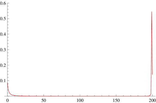
Figure 1: Numerical simulation of H-QW(1) with coin parameter $\gamma_{j}=1/(3+j)$: the horizontal and vertical axes depict position and $\mu_{200}$ with the initial coin state $[1/\sqrt{2},1/\sqrt{2}]$, respectively.

To prove Theorem 3, we prepare the following key lemma with respect to the weight of passage $\Xi_{j}(n)$ in a closed form. We give its proof in the last part of this section.

Lemma 4.

The weight of passage is decomposed into three parts.

$$\Xi_{j}(n)=L_{j}(n)+B_{j}(n)+I_{j}(n),$$ (4.46)

where $L_{j}(n)$, $B_{j}(n)$ and $I_{j}(n)$ are defined in Eqs. (4.61), (4.62) and (4.63), respectively. Moreover for fixed $j$, $\lim_{n\to\infty}I_{j}(n)=\lim_{n\to\infty}I_{n-j}(n)=0$,

$$\lim_{n\to\infty}L_{j}(n) =\sqrt{\frac{r(r-1)}{(r+1)(2r-1)^{2}}}\frac{1}{\sqrt{r+j}}\begin{bmatrix}1/\sqrt{r+1+j}\\ 1/\sqrt{r-1+j}\end{bmatrix}{}^{\dagger}\boldsymbol{l}$$ (4.47)

$$\lim_{n\to\infty}B_{n-j}(n) =-\frac{1}{\sqrt{r(r+1)(r-1)^{4}}}\begin{bmatrix}1\\ 0\end{bmatrix}\left\{\left(\frac{1-r}{r}\right)^{j}{}^{\dagger}\boldsymbol{b}^{E}+\delta_{0}(j){}^{\dagger}\boldsymbol{b}^{0}+\delta_{1}(j){}^{\dagger}\boldsymbol{b}^{1}\right\}$$ (4.48)

and $\lim_{n\to\infty}B_{j}(n)=\lim_{n\to\infty}L_{n-j}(n)=0$.
Here

$$\boldsymbol{b}^{E} =\begin{bmatrix}1-r-r^{2}\\ (r-1)\sqrt{r^{2}-1}\end{bmatrix},\;\boldsymbol{b}^{0}=\begin{bmatrix}2r-1\\ -(r-1)\sqrt{r^{2}-1}\end{bmatrix},\;\boldsymbol{b}^{1}=\begin{bmatrix}1\\ 0\end{bmatrix},\;\boldsymbol{l}=\begin{bmatrix}\sqrt{r-1}\\ \sqrt{r+1}\end{bmatrix}.$$ (4.49)

Remark 2.

From the linear independence of $\boldsymbol{b}^{0}$, $\boldsymbol{b}^{1}$ and $\boldsymbol{b}^{E}\in\mathbb{C}^{2}$, the strongly ballistic spreading, i.e., bottom localization, is always ensured for all initial coin state $\varphi_{0}$ in this walk. On the other hand, choosing an appropriate initial coin state so that $\langle\varphi_{0},\boldsymbol{l}\rangle=0$ eliminates localization at the origin.

Proof of Theorem 3. The first term of RHS in Eq. (4.46), $L_{j}(n)$, contributes localization with power-law around the origin corresponding to part (1) in Theorem 3, while the second term, $B_{j}(n)$, gives the bottom localization corresponding to part (2). The finial term, $I_{j}(n)$, is an intermediate term between first and second terms. Lemma 4 implies that

$$\mu_{\infty}(j)=||\lim_{n\to\infty}L_{j}(n)\varphi_{0}||^{2},\;\widetilde{\mu}_{\infty}(j)=||\lim_{n\to\infty}B_{n-j}(n)\varphi_{0}||^{2}.$$ (4.50)

Algebraic computations of RHS in Eq. (4.50) give desired conclusion.

$\square$

Theorem 4.

1. (Weak convergence)

   $$\frac{X_{n}}{n}\Rightarrow c_{0}\delta_{0}(x)+c_{1}\delta_{1}(x)\;\;\;(n\to\infty),$$ (4.51)

   where $c_{0}=\sum_{j\geq 0}\mu_{\infty}(j)$, $c_{1}=1-c_{0}=\sum_{j\geq 0}\widetilde{\mu}_{\infty}(j)$.

2. (Large deviation type convergence) For the initial state $\varphi$ with $\langle\varphi_{0},\boldsymbol{l}\rangle=0$, we have

   $$\lim_{n\to\infty}\frac{1}{n}\log P\left(1-\frac{X_{n}}{n}>\epsilon\right)=\epsilon\log\left(\frac{1-r}{r}\right)^{2}.$$ (4.52)

Proof.

1. As a consequence of Theorem 3, we immediately obtain part (1).

2. Now we consider

   $$P(1-X_{n}/n>\epsilon)=\sum_{j=[n\epsilon]}^{n}\langle\Xi_{n-j}(n)\varphi_{0},\Xi_{n-j}(n)\varphi_{0}\rangle$$ (4.53)

   for large $n$. The initial state $\langle\varphi_{0},\boldsymbol{l}\rangle=0$ implies that we only estimate $B_{n-j}(n)$ and $I_{n-j}(n)$, that is,

   $$\Xi_{n-j}^{*}(n)\Xi_{n-j}(n)=\\ B_{n-j}^{*}(n)B_{n-j}(n)+I_{n-j}^{*}(n)I_{n-j}(n)+B_{n-j}^{*}(n)I_{n-j}(n)+I_{n-j}^{*}(n)B_{n-j}(n).$$

   We extract the essential parts of $B_{n-j}(n)^{*}B_{n-j}(n)$, $B_{n-j}(n)^{*}I_{n-j}(n)$ and $I_{n-j}(n)^{*}I_{n-j}(n)$ which are directly related to the summation in RHS of Eq. (4.53) as follows:

   $$\left(1-\frac{1}{r+n-j}\right)\tau^{2j},\;\;\frac{\tau^{2j}}{r+n-j},\;\;\mathrm{and}\;\frac{\tau^{2j}}{(r+n-j)(r+n-j+1)},$$

   respectively, where $\tau=(1-r)/r$ (see Eqs. (4.61) and (4.63) for the explicit expressions for $B_{j}(n)$ and $I_{j}(n)$). Put

   $$A_{n,\epsilon}\equiv\sum_{j=[n\epsilon]}^{n}\tau^{2j}\sim\frac{\tau^{2n\epsilon}}{1-\tau^{2}}(1-\tau^{2n(1-\epsilon)}).$$

   Note that

   $$\sum_{j\geq n\epsilon}^{n}\frac{\tau^{2j}}{(r+n-j)(r+n-j+1)}\leq\sum_{j\geq n\epsilon}^{n}\frac{\tau^{2j}}{r+n-j}\leq\frac{1}{r}A_{n,\epsilon}.$$

   Then we have the RHS of Eq. (4.53) is rewritten as

   $$\sum_{j=[n\epsilon]}^{n}\langle\Xi_{n-j}(n)\varphi_{0},\Xi_{n-j}(n)\varphi_{0}\rangle\sim\frac{\tau^{2n\epsilon}}{1-\tau^{2}}\left(1+O(1)\right).$$ (4.54)

   Therefore

   $$\lim_{n\to\infty}\frac{1}{n}\log P(1-X_{n}/n>\epsilon)=\epsilon\log\tau^{2}.$$

∎

Finally, we give the proof of Lemma 4.

Proof of Lemma 4.
At first, we decompose $\Xi_{n-j}(n)$ as $\Xi_{n-j}(n)=\Pi_{L}\Xi_{n-j}(n)+\Pi_{R}\Xi_{n-j}(n)$, where $\Pi_{J}$ is projection onto basis $\boldsymbol{\delta}_{J}$ ($J\in\{L,R\}$). For small $\delta<1$,

$$\Xi_{j}(n)=\frac{1}{2\pi i}\int_{|z|=\delta}\widetilde{\Xi}_{j}(z)\frac{dz}{z^{n+1}}.$$

So we have

$$\Pi_{L}\Xi_{n-j}(n) =\frac{1}{2\pi i}\int_{|z|=\delta}\widetilde{\lambda}^{(+)}_{n-j}\cdots\widetilde{\lambda}^{(+)}_{1}\widetilde{g}^{(+)}_{n-j}\begin{bmatrix}-1/r+z&\sqrt{1-1/r^{2}}\\ 0&0\end{bmatrix}\frac{1}{\widetilde{\Lambda}_{0}}\frac{dz}{z^{n+1}},$$ (4.55)

$$\Pi_{R}\Xi_{n-j}(n) =\frac{1}{2\pi i}\int_{|z|=\delta}\widetilde{\lambda}^{(+)}_{n-j-1}\cdots\widetilde{\lambda}^{(+)}_{1}\begin{bmatrix}0&0\\ -1/r+z&\sqrt{1-1/r^{2}}\end{bmatrix}\frac{1}{\widetilde{\Lambda}_{0}}\frac{dz}{z^{n}}.$$ (4.56)

Since $\widetilde{\lambda}^{(+)}_{j}$ is expressed by

$$\widetilde{\lambda}^{(+)}_{j}=z\sqrt{\frac{r+j-1}{r+j+1}}\frac{(r+j+1)-(r+j)z^{2}}{(r+j)-(r+j-1)z^{2}},$$

we obtain

$$\widetilde{\lambda}^{(+)}_{j}\cdots\widetilde{\lambda}^{(+)}_{1}=\frac{1+1/r}{z^{2}-(r+1)/r}\left\{\sqrt{\frac{r+j}{r+j-1}}-z^{2}\sqrt{\frac{r+j-1}{r+j}}\right\}z^{j-1}.$$ (4.57)

Moreover

$$\frac{1}{\widetilde{\Lambda}_{0}}=\frac{-r^{2}}{1-r^{2}}\frac{z^{2}-\frac{r+1}{r}}{\left(z-\frac{r}{1-r}\right)(z-1)}.$$ (4.58)

Substituting Eqs. (4.57) and (4.58) into Eqs. (4.55) and (4.56),

$$\Pi_{L}\Xi_{n-j}(n)=\frac{-\sqrt{\frac{r^{3}}{(r-1)^{2}(r+1)}}}{\sqrt{(r+n-j+1)(r+n-j)}}\\ \times\int_{|z|=\delta}\frac{1}{\left(z-\frac{r}{r+1}\right)(z-1)}\begin{bmatrix}-1/r+z&\sqrt{1-1/r^{2}}\\ 0&0\end{bmatrix}\frac{dz}{2\pi iz^{j-1}},$$ (4.59)

$$\Pi_{R}\Xi_{n-j}(n)=\sqrt{\frac{r^{3}}{(r-1)^{2}(r+1)}}\sqrt{1-\frac{1}{r+n-j}}\\ \times\int_{|z|=\delta}\left\{\frac{z+1}{z-\frac{r}{1-r}}-\frac{1}{r+n-j-1}\frac{1}{\left(z-\frac{r}{1-r}\right)(z-1)}\right\}\\ \begin{bmatrix}0&0\\ -1/r+z&\sqrt{1-1/r^{2}}\end{bmatrix}\frac{dz}{2\pi iz^{j+1}}.$$ (4.60)

Direct computations of the residues at $z=0$ in the integrands of RHSs of Eqs. (4.59) and (4.60), respectively, lead to

$$\Xi_{j}(n)=B_{j}(n)+L_{j}(n)+I_{j}(n),$$

where

$$B_{n-j}(n)=-\sqrt{1-\frac{1}{r+n-j}}\frac{1}{\sqrt{r(r+1)(r-1)^{4}}}\begin{bmatrix}1\\ 0\end{bmatrix}\\ \times\left\{\left(\frac{1-r}{r}\right)^{j}{}^{\dagger}\boldsymbol{b}^{E}+\delta_{0}(j){}^{\dagger}\boldsymbol{b}^{0}+\delta_{1}(j){}^{\dagger}\boldsymbol{b}^{1}\right\},$$ (4.61)

$$L_{j}(n) =\sqrt{\frac{r(r-1)}{(r+1)(2r-1)^{2}}}\frac{1}{\sqrt{r+j}}\begin{bmatrix}1/\sqrt{r+1+j}\\ 1/\sqrt{r-1+j}\end{bmatrix}{}^{\dagger}\boldsymbol{l},$$ (4.62)

$$I_{j}(n) =\frac{\left(\frac{1-r}{r}\right)^{n-j}}{\sqrt{r+j}}\begin{bmatrix}r^{3}/((r-1)^{4}(2r-1)^{2}(r+1))\cdot 1/\sqrt{r+j+1}\\ 1/\sqrt{r(r+1)}\cdot 1/\sqrt{r+j-1}\end{bmatrix}{}^{\dagger}\boldsymbol{b}^{E}.$$ (4.63)

Obviously, from Eqs. (4.61), (4.62) and (4.63), we obtain $\lim_{n\to\infty}I_{j}(n)=\lim_{n\to\infty}I_{n-j}(n)=\lim_{n\to\infty}B_{j}(n)=\lim_{n\to\infty}L_{n-j}(n)=0$, and

$$\lim_{n\to\infty}L_{j}(n) =\sqrt{\frac{r(r-1)}{(r+1)(2r-1)^{2}}}\frac{1}{\sqrt{r+j}}\begin{bmatrix}1/\sqrt{r+1+j}\\ 1/\sqrt{r-1+j}\end{bmatrix}{}^{\dagger}\boldsymbol{l},$$

$$\lim_{n\to\infty}B_{n-j}(n) =-\frac{1}{\sqrt{r(r+1)(r-1)^{4}}}\begin{bmatrix}1\\ 0\end{bmatrix}\left\{\left(\frac{1-r}{r}\right)^{j}{}^{\dagger}\boldsymbol{b}^{E}+\delta_{0}(j){}^{\dagger}\boldsymbol{b}^{0}+\delta_{1}(j){}^{\dagger}\boldsymbol{b}^{1}\right\}.$$

We complete the proof.

$\square$

5 Summary and Discussion

We considered a connection between the Schur function which gives the spectrum of the CMV matrix and a generating function of QWs (Lemma 3). We presented an application of this relationship to analysis of stochastic behavior of QWs (Section 4). In the H-QW(1) with parameters defined by Eq. (4.39), we showed that opposite properties happen simultaneously, that is, localization with a power-law decay around the origin and an “extreme” ballistic spreading called bottom localization.

Finally, we discuss the second kind of QW on the half line corresponding to the first kind of QW discussed in Sect. 4. As we will see below, the non existence of just one self loop at the origin has large effect on a behavior of the bottom localization. Indeed, from a similar fashion of Sect. 4, applying Lemmas 2 and 3 to H-QW(2), we have the following limit theorem corresponding to Theorem 3.

Theorem 5.

Limit theorems for H-QW(2)

1. (Localization around the origin)

   $$\lim_{n\to\infty}\mu_{n}(j)\sim\frac{1+(-1)^{n+j}}{2}\times\begin{cases}\left(\frac{1}{r+1}\right)^{2}&\text{: $j=0$,}\\ \frac{{2r}/(r+1)}{(r-1+j)(r+1+j)}&\text{: $j\geq 1$}\end{cases}$$ (5.64)

2. (Localization around the bottom)

   $$\lim_{n\to\infty}\widetilde{\mu}_{n}(j)=\left(1-\frac{1}{1+r}\right)\delta_{0}(j).$$ (5.65)

Moreover $c_{0}+c_{1}=1$, with $c_{0}=\sum_{j\geq 0}\lim_{n\to\infty}\mu_{n}(j)$, $c_{1}=\sum_{j\geq 0}\lim_{n\to\infty}\widetilde{\mu}_{n}(j)$.

Therefore, the contribution of the bottom localization for H-QW(2) is just nothing but the weight of “right $\to$ right $\to\cdots$ ” path itself. We leave the doubly infinite case to the readers applying Lemmas 2 and 3.

Acknowledgments. NK acknowledges financial support of the Grant-in-Aid for Scientific Research (C) of Japan Society for the Promotion of Science (Grant No. 21540118). ES’s work was partially supported by the Grant-in-Aid for Young Scientists (B) of Japan Society for the Promotion of Science (Grant No. 25800088).

References

- [1] D. Meyer, From quantum cellular automata to quantum lattice gases, Journal of Statistical Physics 85 (1996) 551-574.
- [2] R. F. Feynman, A. R. Hibbs, Quantum Mechanics and Path Integrals, McGraw-Hill, Inc., New York, 1965.
- [3] S. P. Gudder, Quantum Probability, Academic Press, 1988.
- [4] M. J. Cantero, F. A. Grünbaum, L. Moral, L. Velázquez, The CGMV method for quantum walks, Quantum Inf. Process. 11 (2012) pp.1149–1192.
- [5] A. Bressler, R. Pemantle, Quantum random walks in one dimension via generating functions, Proceedings of the 2007 Conference on Analysis of Algorithms (2007).
- [6] K. Chisaki, M. Hamada, N. Konno and E. Segawa, Limit theorems for discrete-time quantum walks on Trees, Interdisciplinary Information Sciences 15 (2009), 423-429.
- [7] K. Chisaki, N. Konno, E. Segawa, Limit theorems for the discrete-time quantum walk on a graph with joined half lines, Quantum Information and Computation, 12 (2012) 0314–0333
- [8] N. Konno, T. Łuczak, E. Segawa, Limit measures of inhomogeneous discrete-time quantum walks in one dimension, Quantum Inf. Process. 12 (2013) pp.33–53.
- [9] C. Liu, N. Petulante, A weak limit theorem for quantum walks on the half-line arxiv:1212.1109.
- [10] N. Konno, E. Segawa, Localization of discrete time quantum walks on a half line via the CGMV method, Quantum Inf. Comput. 11 (2011), pp.485–495.
- [11] N. Konno, Quantum random walks in one dimension, Quantum Inf. Proc. 1, 345-354 (2002),
- [12] N. Konno, A new type of limit theorems for the one-dimensional quantum random walk, J. Math. Soc. Jpn. 57, 1179-1195 (2005).
- [13] A. Joye and M. Merkli, Dynamical localization of quantum walks in random environments, J. Stat. Phys. 140 (2010), 1023–1053.
- [14] A. Ahlbrecht, V. B. Scholz and A. H. Werner, Disordered quantum walks in one lattice dimension, J. Math. Phys. 52 (2011), 102201.
- [15] F.A. Grünbaum, L. Velázquez, The quantum walk of F. Riesz, Proceedings of FoCAM2011, London Mathematical Society Lecture Notes Series, 403, pp.93–112 (2012).
- [16] M. J. Cantero, L. Moral and L. Velázquez, Five-diagonal matrices and zeros of orthogonal polynomials on the unit circle, Linear Algebra and its Applications, 362 (2003), 29-56.
- [17] M. J. Cantero, L. Moral and L. Velázquez (2005), Minimal representations of unitary operators and orthogonal polynomials on the unit circle, Linear Algebra and its Applications, 405, 40-65.
- [18] M. J. Cantero, F. A. Grünbaum, L. Moral and L. Velázquez (2010), Matrix valued Szegö polynomials and quantum walks, Communications on Pure and Applied Mathematics, 63, 464-507.
- [19] B. Simon, Orthogonal Polynomials on the Unit Circle, Part 1: Classical Theory, AMS Colloq.Publ., 54, AMS, Providence, RI (2005).
- [20] M. Stefanak, T. Kiss, I. Jex, Recurrence of biased quantum walks on a line, New. J. Phys. 11, 043027 (2009)
- [21] F.A. Grünbaum, L. Velázquez, A. Werner, R.F. Werner, Recurrence for discrete time unitary evolutions, Commun. Math. Phys. (to appear, available online), DOI10.1007/s00220-012-1645-2 (2013).
- [22] J. Bourgain, F.A. Grünbaum, L. Velázquez, J. Wilkening, Quantum recurrence of a subspace and operator-valued Schur functions, arXiv:1302.7286.