Noisy continuous time random walks

Abstract

Experimental studies of the diffusion of biomolecules in the environment of biological cells are routinely confronted with multiple sources of stochasticity, whose identification renders the detailed data analysis of single molecule trajectories quite intricate. Here we consider subdiffusive continuous time random walks, that represent a seminal model for the anomalous diffusion of tracer particles in complex environments. This motion is characterized by multiple trapping events with infinite mean sojourn time. In real physical situations, however, instead of the full immobilization predicted by the continuous time random walk model, the motion of the tracer particle shows additional jiggling, for instance, due to thermal agitation of the environment. We here present and analyze in detail an extension of the continuous time random walk model. Superimposing the multiple trapping behavior with additive Gaussian noise of variable strength, we demonstrate that the resulting process exhibits a rich variety of apparent dynamic regimes. In particular, such noisy continuous time random walks may appear ergodic while the naked continuous time random walk exhibits weak ergodicity breaking. Detailed knowledge of this behavior will be useful for the truthful physical analysis of experimentally observed subdiffusion.

I Introduction

In a series of experiments in the Weitz lab at Harvard, Wong et al. wong observed that the motion of plastic tracer microbeads in a reconstituted mesh of cross-linked actin filaments is characterized by anomalous diffusion of the form

$$\langle\mathbf{r}^{2}(t)\rangle=\int\mathbf{r}^{2}P(\mathbf{r},t)d\mathbf{r}\simeq K_{\alpha}t^{\alpha}$$ (1)

of the ensemble averaged mean squared displacement (MSD). Here, $K_{\alpha}$ is the anomalous diffusion exponent of physical dimension $[K_{\alpha}]=\mathrm{cm}^{2}/\mathrm{sec}^{\alpha}$, and the anomalous diffusion exponent $\alpha$ is in the subdiffusive range $0<\alpha<1$. $P(\mathbf{r},t)$ is the probability density function to find the test particle at position $\mathbf{r}$ at time $t$. Wong et al. demonstrated that the motion of the microbeads is represented by a random walk with subsequent immobilization events of the beads in ‘cages’ within the network wong . The durations $\tau$ of these immobilization periods were shown to follow the distribution

$$\psi(\tau)\sim\frac{\tau_{0}^{\alpha}}{\tau^{1+\alpha}},$$ (2)

with the scaling exponent $\alpha$. The exponent $\alpha$ turns out to be a function of the ratio between the bead size and the typical mesh size. Thus, when the bead size is larger than the mesh size, the bead becomes fully immobilized, $\alpha=0$. Conversely, when the bead is much smaller than the typical mesh size, it moves like a Brownian particle [$\alpha=1$, in Eq. (1)], almost undisturbed by the actin mesh. However, when the bead size is comparable to the mesh size, the motion of the bead is impeded by the mesh, giving rise to a saltatory bead motion in between cages. While the measured distribution (2) of immobilization times indeed captures the statistics of the long time movement of the beads, the measured trajectories also exhibit an additional noise, superimposed to the jump motion according to the law (2) wong . This additional noise is visible as jiggling around a typical position during sojourn periods of the bead, and appears like regular white noise.

Above example is representative for the task of physical analysis of single particle tracking experiments. Indeed, following single particles such as large labeled molecules, viruses, or artificial tracers in the environment of living cells has become a standard technique in many laboratories, since it reveals the individual trajectories without the problem of ensemble averaging. However, the large amount of potentially noisy data also poses a practical challenge. In physics and mathematics ideal stochastic processes have been investigated for many years, including Brownian motion, fractional Brownian motion, continuous time random walks, Lévy flights, etc. While these can be reasonable approximations for the physical reality, they rarely represent the whole story. In many cases, a superposition of at least two types of stochastic motion are found, such as the ‘contamination’ of the pure stop-and-go motion described by the waiting time distribution (2) with additional noise in the above example of the tracer beads in the actin mesh. Similarly, Weigel et al. in their study of protein channel motion in the walls of living human kidney cells observed a superposition of stochastic motion governed by the law (2) and motion patterns corresponding to diffusion on a fractal weigel . Tabei et al. show that the motion of insulin granules in living MIN6 cells is best explained by a hybrid model in which fractional Brownian motion is subordinated to continuous time random walk subdiffusion tabei . Finally, Jeon et al. find that the motion of lipid granules in living yeast cells is governed by continuous time random walk motion at short times, turning over to fractional Brownian motion at longer times lene . Even if the trajectories are ideal, in the lab we always have to deal with additional sources of noise, for instance, the motion within the sample may become disturbed by a slow, random drift of the object stage in the microscope setup, or simply by the diffusive motion on the cover slip of a living cell, inside which the actual motion occurs that we want to follow.

In recent years a tool box for data analysis was developed by several groups, in particular, in the context of diffusion of tracers in the microscopic cellular environment. These also include fundamental aspects of statistical physics such as the ergodic properties of the underlying process and the irreproducible nature of the time averages of the data pt . However, to the best of our knowledge these analysis methods and the fundamental properties of statistical mechanics (that is, ergodicity) have not been tested in the presence of additional noise. For instance, if we encounter a non-ergodic process superimposed with an ergodic one, as defined precisely below, what will we find as the result of such an experiment? Here we develop and study in detail a new framework for the motion of a test particle, the noisy continuous time random walk (nCTRW) subject simultaneously to a power-law distribution (2) of sojourn times and additional Gaussian noise. Interestingly, the noise turns out to have a dramatic effect on the time averaged MSD, typically evaluated in single particle tracking experiments, but a trivial effect on the ensemble averaged MSD. We hope that this contribution will be a step towards more realistic modeling of trajectories of single molecules, but also of other diffusive motions of particles in complex environments.

Our analysis is based on two different scenarios for the additional Gaussian noise. Thus, we will consider (i) a regular diffusive motion on top of the power-law sojourn times (2). This scenario mirrors effects such as the diffusion on the cover slip of the biological cell, in which the actual motion occurs that we want to monitor. (ii) We study an Ornstein-Uhlenbeck noise with a typical amplitude which may reflect an intrinsically noisy environment, such as in the case of the tracer beads in the actin network. We will study the MSD of the resulting motion both in the sense of the conventional ensemble average and, for its relevance in the analysis of single particle tracking measurement, the time average. Moreover we demonstrate how a varying strength of the additional noise may blur the result of stochastic diagnosis methods introduced recently, such as the scatter of amplitudes of time averaged MSDs around the average over an ensemble of trajectories, or the $p$-variation method.

The paper is organized as follows. In Sec. II.1, we briefly discuss the concepts of anomalous diffusion and single particle tracking along with the role of (non-)ergodicity in the context of ensemble versus time averaged MSDs. In Sec. II.2 we review some methods of single particle tracking analysis. Section III then introduces our nCTRW model consisting of a random walk with long sojourn times superimposed with Gaussian noise, and we explain the simulation scheme. The main results and discussions are presented in Secs. IV and V: in Sec. IV, we study the statistical behavior of nCTRW motion in the presence of superimposed free Brownian motion, while Sec. V is devoted to the motion disturbed by Ornstein-Uhlenbeck noise. Finally, the conclusions and an outlook are presented in Sec. VI. In the Appendix, we provide a brief outline of the stochastic analysis tools used to quantify the nCTRW processes studied in Secs. IV and V. Note that in the following, for simplicity we concentrate on the one-dimensional case; all results can easily be generalized to higher dimensions.

II Anomalous diffusion and single particle tracking

In this Section we briefly review the continuous time random walk (CTRW) model and the behavior of CTRW time series. Moreover, we present some common methods to analyze traces obtained from single particle tracking experiments or simulations.

II.1 Continuous time random walks and time averaged mean squared displacement

Anomalous diffusion of the subdiffusive form (1) with $0<\alpha<1$ is quite commonly observed in a large variety of systems and on many different scales havlin ; bouchaud ; report ; report1 . Examples range from microscopic systems such as the motion of small tracer particles in living biological cells and similar crowded systems golding ; hoefling ; saxton1 , over the motion of charge carriers in amorphous semiconductors scher to the dispersion of chemical tracers in groundwater systems grl .

A prominent model to describe the subdiffusion law (1) is given by the Montroll-Weiss-Scher continuous time random walk (CTRW) montroll ; scher . Originally applied to describe extensive data from the stochastic motion of charge carriers in amorphous semiconductors scher , the CTRW model finds applications in many areas. Inter alia, CTRW subdiffusion was shown to underlie the motion of microbeads in reconstituted actin networks wong , the subdiffusion of lipid granules in living yeast cells lene ; natascha of protein channels in human kidney cells weigel , and insulin granules in MIN6 cells tabei , as well as the temporal spreading of tracer chemicals in groundwater aquifers grl ; brian . While the sojourn times in a subdiffusive CTRW follow the law (2), the length of individual jumps is governed by a distribution $\lambda(x)$ of jump lengths, with finite variance $\sigma^{2}=\int x^{2}\lambda(x)dx$. In the simplest case of a jump process on a lattice, each jump is of the length of the lattice constant. Physically, the power-law form (2) of sojourn times may arise due to multiple trapping events in a quenched energy landscape with exponentially distributed depths of traps monthus ; burov . Subdiffusive CTRWs macroscopically exhibit long-tailed memory effects, as characterized by the dynamic equation for the probability density function $P(x,t)$ containing fractional differential operators, see below mebakla .

Usually, we think in terms of the ensemble average (1) when we talk about the MSD of a diffusive process. However, starting with Ivar Nordlund’s seminal study of the Brownian motion of a slowly sedimenting mercury droplet nordlund and now routinely performed even on the level of single molecules wong ; golding ; lene ; natascha ; weigel ; tabei ; weber ; sm ; bronstein ; szymansky ; natascha1 ; caspi ; banks , the time series $x(t)$ obtained from measuring the trajectory of an individual particle is evaluated in terms of the time averaged MSD

$$\overline{\delta^{2}(\Delta)}=\frac{1}{T-\Delta}\int_{0}^{T-\Delta}\Big{(}x(t+\Delta)-x(t)\Big{)}^{2}dt$$ (3)

where $\Delta$ is the so-called lag time, and $T$ is the overall measurement time. For Brownian motion, the time averaged MSD (3) is equivalent to the ensemble averaged MSD (1), $\langle x^{2}(\Delta)\rangle=\overline{\delta^{2}(\Delta)}$, if only the measurement time $T$ is sufficiently long to ensure self-averaging of the process along the trajectory. This fact is a direct consequence of the ergodic nature of Brownian motion pt ; stas2 . To obtain reliable behaviors for the time averaged MSD for trajectories with finite $T$ one often introduces the average

$$\left<\overline{\delta^{2}(\Delta)}\right>=\frac{1}{N}\sum_{i=1}^{N}\overline{\delta^{2}_{i}(\Delta)}$$ (4)

over several individual trajectories $\overline{\delta^{2}_{i}(\Delta)}$.

What happens when the process is anomalous, of the form (1)? There exist anomalous diffusion processes, that are ergodic in the above sense that for sufficiently long $T$ we observe the equivalence $\langle x^{2}(\Delta)\rangle=\overline{\delta^{2}(\Delta)}$. Prominent examples are given by diffusion on random fractal geometries yasmin , as well as fractional Brownian motion and the related fractional Langevin equation motion for which ergodicity is approached algebraically deng ; igorg ; jae . Such behavior was in fact corroborated in particle tracking experiments in crowded environments szymansky ; bronstein ; natascha1 and simulations of lipid bilayer systems kneller ; matti . In superdiffusive Lévy walks time and ensemble averaged MSDs differ merely by a factor lws ; zukla ; froemberg . However, the diverging sojourn time in the subdiffusive CTRW processes naturally causes weak ergodicity breaking in the sense that even for extremely long measurement times $T$ ensemble and time averages no longer coincide bouchaud1 ; barkai ; zaid . For the time averaged MSD the consequences are far-reaching. Thus, for subdiffusive CTRW we find the somewhat counterintuitive result that the time averaged MSD for free motion scales linearly with the lag time, $\langle\overline{\delta^{2}(\Delta,T)}\rangle\simeq K_{\alpha}\Delta/T^{1-\alpha}$ for $\Delta\ll T$, and thus $\langle x^{2}(\Delta)\rangle\neq\overline{\delta^{2}(\Delta)}$ He ; lubelski . In particular, the result $\langle\overline{\delta^{2}(\Delta)}\rangle$ decreases with the measurement time $T$, an effect of ageing. Concurrently, the MSD of subdiffusive CTRWs depends on the time difference between the preparation of the system and the start of the measurement johannes . Under confinement, while the ensemble averaged MSD saturates towards the thermal value, the time averaged MSD continues to grow as $\langle\overline{\delta^{2}(\Delta)}\rangle\simeq\Delta^{1-\alpha}$ as long as $\Delta\ll T$ stas1 ; neusius . Another important consequence of the weakly non-ergodic behavior is that the time averaged MSD (3) remains irreproducible even in the limit of $T\rightarrow\infty$: the amplitude of individual time averaged MSD curves $\overline{\delta^{2}_{i}(\Delta)}$ scatters significantly between different trajectories, albeit with a well-defined distribution He ; igor . In other words, this scatter of amplitudes corresponds to a distribution of diffusion constants saxton2 . Active transport of molecules in the cell exhibits superdiffusion with non-reproducible results for the time averages caspi2 , a case treated theoretically only recently lws ; froemberg ; akimoto .

To pin down a given stochastic mechanism underlying some measured trajectories, several diagnosis methods have been developed. Thus, one may analyze the first passage behavior olivier , moment ratios and the statistics of mean maximal excursions vincent , the velocity autocorrelation stas2 ; matti , the statistics of the apparent diffusivities radons , or the $p$-variation of the data marcin ; kepten . In the following we analyze the sensitivity of the time averaged MSD and its amplitude scatter as well as the $p$-variation method to noise, that is superimposed to naked subdiffusive CTRWs. In particular, we show that at larger amplitudes of the additional noise the CTRW-inherent weak non-ergodicity may become completely masked.

II.2 A primer on single particle trajectory analysis

Before proceeding to define the nCTRW process, we present a brief review of several techniques developed recently for the analysis of single particle trajectories.

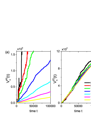
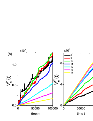
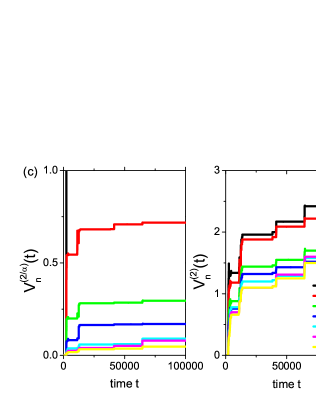
Figure 1: Results of $p$-variation test for (a) Brownian noise $z_{B}(t)$, (b) Ornstein-Uhlenbeck noise $z_{OU}(t)$, and (c) subdiffusive CTRW $x_{\alpha}(t)$ with $\alpha=0.5$. The left panels in each case are for $p=4$ for both (a) and (b), and (c) $p=2/\alpha=4$. All right panels are for $p=2$. The color coding refers to the values of $n$ indicated in the right panel of each pair of graphs.

II.2.1 Mean squared displacement

Already from the time averaged MSD $\overline{\delta^{2}_{i}}$ of individual particle traces important information on the nature of the process may be extracted, provided that the measurement time $T$ is sufficiently long. Thus, for ergodic processes the time and ensemble averaged MSD are equivalent, $\langle\overline{\delta^{2}(\Delta)}\rangle=\langle x^{2}(\Delta)\rangle$. A significant difference between both quantities points at non-ergodic behavior. In particular, the scatter of amplitudes (distribution of diffusion constants) between individual traces $\overline{\delta^{2}_{i}}$ turns out to be a quite reliable measure for the (non-)ergodicity of a process. Thus, in terms of the dimensionless parameter $\xi=\overline{\delta^{2}}/\langle\overline{\delta^{2}}\rangle$ the distribution of amplitudes $\phi(\xi)$ has a Gaussian profile centered on the ergodic value $\xi=1$ for finite-time ergodic processes jeon . Its width narrows with increasing $T$, eventually approaching the sharp distribution $\delta(\xi-1)$ at $T\to\infty$, i.e., each trajectory gives exactly the same result, equivalent to the ensemble averaged MSD. For subdiffusive CTRW processes $\phi(\xi)$ is quite broad and has a finite value at $\xi=0$ for completely stalled trajectories stas2 ; He ; jeon ; johannes ; heinsalu . For $\alpha\leq 1/2$ the maximum of the distribution is at $\xi=0$, while for $\alpha>1/2$ the maximum is located at $\xi=1$. The non-Gaussian distribution $\phi(\xi)$ for subdiffusive CTRWs is almost independent of $T$, and its shape is already well established even for relatively short trajectories jeon .

II.2.2 $p$-variation test

The $p$-variation test was recently promoted as a tool to distinguish CTRW and FBM-type subdiffusion marcin . It is defined in terms of the sum of increments of the trajectory $x(t)$ on the interval $[0,T]$ as

$$V_{n}^{(p)}(t)=\sum_{j=0}^{2^{n}-1}\left|x\left(\frac{(j+1)T}{2^{n}}\wedge t\right)-x\left(\frac{jT}{2^{n}}\wedge t\right)\right|^{p},$$ (5)

where $a\wedge b=\mathrm{min}\{a,b\}$. The quantity $V^{(p)}=\lim_{n\to\infty}V_{n}^{(p)}$ has distinct properties for certain stochastic processes. Thus, for both free and confined Brownian motion $V^{(2)}(t)\sim t$ and $V^{(p)}(t)=0$ for any $p>2$. For fractional Brownian motion, $V^{(2)}(t)=\infty$, while $V^{(2/\alpha)}(t)\sim t$. Finally, for CTRW subdiffusion, $V^{(2)}(t)$ features a step-like, monotonic increase as function of time $t$, and $V^{(2/\alpha)}(t)=0$.

Fig. 1 shows the $p$-variation results for Brownian noise $z_{B}(t)$, Ornstein-Uhlenbeck noise $z_{OU}(t)$, and the naked subdiffusive CTRW $x_{\alpha}(t)$. We plot the sum (5) for various, finite values of $n$. For the Brownian noise $z_{B}(t)$, $V_{n}^{(4)}$ monotonically decreases with growing $n$, a signature of the predicted convergence to $V^{(4)}\rightarrow 0$. The sum $V^{(2)}$ appears independent of $n$ and proportional to time $t$, as expected. For the Ornstein-Uhlenbeck noise $z_{OU}(t)$ we observe that $V^{(4)}$ scales linearly with $t$ and the slope decreases with growing $n$, indicating a convergence to zero. Also $V^{(2)}$ is linear in $t$. For smaller $n$, the slope increases with $n$ and saturates at large $n$. Finally, for CTRW subdiffusion $V^{(2/\alpha)}$ appears to converge to zero for increasing $n$, as predicted. In contrast, $V^{(2)}$ has the distinct, monotonic step-like increase expected for CTRW subdiffusion. A more detailed description of the $p$-variation for Ornstein-Uhlenbeck noise and CTRW subdiffusion is found in Appendix A.

III Noisy continuous time random walk

In this Section we define the nCTRW model and describe our simulations scheme used in the following Sections.

III.1 Two nCTRW models

We consider an nCTRW process $x(t)$ in which ordinary CTRW subdiffusion $x_{\alpha}(t)$ with anomalous diffusion exponent $0<\alpha<1$ is superimposed with the Gaussian noise $\eta z(t)$,

$$x(t)=x_{\alpha}(t)+\eta z(t).$$ (6)

That means that the Gaussian process $z(t)$ is additive and thus independent of $x_{\alpha}(t)$. The relative strength of the additional Gaussian noise is controlled by the amplitude parameter $\eta\geq 0$. In this study we consider the following two Gaussian processes: (1) in the first case $z(t)$ is a simple Brownian diffusive process $z_{B}(t)$ with zero mean $\langle z_{B}(t)\rangle=0$ and variance $\langle z_{B}^{2}(t)\rangle=2Dt$. As mentioned, physically this could represent the (slow) diffusion of a living bacteria or endothelial cell on the cover slip while we want to record the motion of a tracer inside the cell, or the random drifting of the experimental stage. (2) In the second case $z(t)$ represents Ornstein-Uhlenbeck process $z_{OU}(t)$, the confined Brownian motion in an harmonic potential (see Eq. (18) for the definition of the process). Stochastic processes of this second kind, for example, likely mimic the motion of a bead confined in a polymer network or immersed in a macromolecularly crowded environment, where the thermal agitation of the confining environment gives rise to the random fluctuation of the position of the trapped tracer particle around some average value.

According to the definition (6), nCTRW possesses have the following generic properties. Its probability density function (PDF) $P(x,t)$ is given by the convolution of the individual PDFs $P_{\alpha}(x,t)$ of a CTRW subdiffusion process and $P_{G}(x,t)$ of the Gaussian process,

$$P(x,t)=\int_{-\infty}^{\infty}P_{\alpha}(x-y,t)P_{G}(y,t)dy.$$ (7)

This chain rule states that a given position $x$ of the combined process is given by the product of the probability that the CTRW process has reached the position $x-y$ and the Gaussian process contributes the distance $y$, or vice versa. Here the PDF $P_{\alpha}(x,t)$ satisfies the fractional Fokker-Planck equation report

$$\frac{\partial}{\partial t}P_{\alpha}(x,t)={{}_{0}}\mathcal{D}_{t}^{1-\alpha}K_{\alpha}\frac{\partial^{2}}{\partial x^{2}}P_{\alpha}(x,t)$$ (8)

where the Riemann-Liouville fractional derivative of $P(x,t)$ is

$${}_{0}\mathcal{D}_{t}^{1-\alpha}P_{\alpha}(x,t)=\frac{1}{\Gamma(\alpha)}\frac{\partial}{\partial t}\int_{0}^{t}\frac{P_{\alpha}(x,t^{\prime})}{(t-t^{\prime})^{1-\alpha}}dt^{\prime}.$$ (9)

Physically, this fractional operator thus represents a memory integral with a slowly decaying kernel. From definition (6) it follows that the ensemble averaged MSD is given by

$$\langle x^{2}(t)\rangle = \int_{-\infty}^{\infty}x^{2}P_{\alpha}(x,t)dx+\int_{-\infty}^{\infty}y^{2}P_{G}(y,t)dy$$ (10)

$$= \langle x_{\alpha}^{2}(t)\rangle+\eta^{2}\langle z^{2}(t)\rangle.$$

The characteristic function of $P(x,t)$ according to Eq. (7) is given by the product

$$P(q,t)=\int_{-\infty}^{\infty}e^{iqx}P(x,t)dx=P_{\alpha}(q,t)P_{G}(q,t)$$ (11)

of the characteristic functions of the individual processes, $P_{\alpha}$ and $P_{G}$. We here use the simplified notation that the Fourier transform of a function is expressed by its explicit dependence on the Fourier variable $q$. With the Mittag-Leffler function $E_{\alpha}(x)=\sum_{m=0}^{\infty}x^{m}/\Gamma(1+\alpha m)$ we find that report

$$P_{\alpha}(q,t)=E_{\alpha}\left(-q^{2}K_{\alpha}t^{\alpha}\right),$$ (12)

assuming that the CTRW process starts at $t=0$ with initial conditions $x_{\alpha}(0)=0$. The characteristic function $P_{\alpha}(q,t)$ initially decays like a stretched exponential $P_{\alpha}(q,t)\approx\exp(-q^{2}K_{\alpha}t^{\alpha}/\Gamma(1+\alpha))$ and has the asymptotic power-law decay $P_{\alpha}(q,t)\sim 1/(q^{2}K_{\alpha}t^{\alpha})$.

The Brownian noise $\eta z_{B}(t)$ with initial condition $z_{B}(0)=0$ has the characteristic function

$$P_{G}(q,t)=\exp\left(-\eta^{2}Dq^{2}t\right).$$ (13)

In the nCTRW process this Brownian noise always dominates the dynamics of the process at long times, since the exponential relaxation (13) dominates the characteristic function $P(q,t)$. The Ornstein-Uhlenbeck noise $\eta z_{OU}(t)$ with $z_{OU}(0)=0$, defined in Eq. (18), has the characteristic function

$$P_{G}(q,t)=\exp\left(-\frac{\eta^{2}Dq^{2}}{2k}\left(1-e^{-2kt}\right)\right).$$ (14)

At short times $t\ll k^{-1}$ when confinement by the harmonic Ornstein-Uhlenbeck potential is negligible, Eq. (14) reduces to the result (13) for Brownian noise, and thus the characteristic functions of the two nCTRW processes are identical. At longer times the characteristic function (14) saturates to $P_{G}(q)=\exp[-\eta^{2}Dq^{2}/(2k)]$. This means that the long-time behavior of the nCTRW with superimposed Ornstein-Uhlenbeck noise, largely reflects the naked CTRW process $x_{\alpha}(t)$, if the noise level is not too high. Keeping these general features in mind, we further study the statistical quantities of the two nCTRW processes numerically.

III.2 Simulation of the nCTRW process

To simulate the nCTRW process we independently obtain time traces of the subdiffusive CTRW motion $x_{\alpha}(t)$ and the additional Gaussian noise. The motion $x_{\alpha}(t)$ with $0<\alpha<1$ is generated on a lattice of spacing $a$ from the normalized waiting time distribution

$$\psi(\tau)=\frac{\alpha/\tau_{0}}{(1+\tau/\tau_{0})^{1+\alpha}}$$ (15)

with the power-law asymptotic scaling $\psi(\tau)\sim\alpha\tau_{0}^{\alpha}/\tau^{1+\alpha}$. Here $\tau_{0}$ is a scaling constant of dimension $[\tau_{0}]=\mathrm{sec}$. The jump lengths are determined by the $\delta$-distribution $\lambda(x)=\frac{1}{2}\delta(|x|-a)$ lene ; jae . Within this construction the CTRW process is associated with the fractional Fokker-Planck equation (8) with the anomalous diffusion exponent eli

$$K_{\alpha}=\frac{\Gamma(1-\alpha)a^{2}}{2\tau_{0}^{\alpha}}.$$ (16)

In the simulations we choose $\tau_{0}=1$, and consequently in the following times are given in units of $\tau_{0}$, which is also chosen equal to the time increments $\delta t$, at which the system is updated. The lattice spacing is $a=0.1$. We simulate the cases $\alpha=0.5$ and $0.8$.

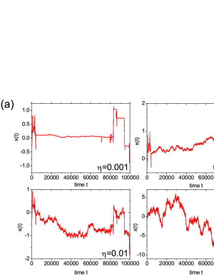
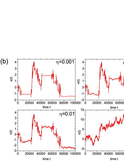
Figure 2: Sample trajectories of the nCTRW process $x_{\alpha}(t)$ with superimposed Brownian noise $\eta z_{B}(t)$ of strength $\eta$, for several values of $\eta$, and for anomalous diffusion exponents (a) $\alpha=0.5$ and (b) $\alpha=0.8$. With increasing noise strength the otherwise pronounced sojourn states become increasingly blurred by the Brownian motion. For each $\alpha$ the CTRW part of the trajectory is identical.

The added Gaussian noise is obtained as follows. Brownian noise $z(t)=z_{B}(t)$ is obtained at discrete times $t_{n}=n\delta t$ (with $\delta t=1$), in terms of the Brownian walk

$$z_{B}(t_{n})=\sum_{k=1}^{n}\delta t\sqrt{2D}\xi_{B}(t_{k}),$$ (17)

where $\xi_{B}(t)$ represents white Gaussian noise of zero mean and unit variance $1/\delta t$ with our choice $\delta t=1$. In the simulations we take $D=0.05$, such that $\langle z_{B}^{2}(1)\rangle=0.1$. The Ornstein-Uhlenbeck noise $z(t)=z_{OU}(t)$ is obtained by integration of the Langevin equation

$$\frac{d}{dt}z_{OU}(t)=-kz_{OU}(t)+\sqrt{2D}\xi_{B}(t)$$ (18)

with the initial condition $z_{OU}(0)=0$. Here, the coefficient of the restoring force is chosen as $k=0.01$. For both Brownian and Ornstein-Uhlenbeck noise, the following values for the noise strength are used: $\eta=0.001$, $0.005$, $0.01$, and $0.1$.

IV nCTRW with Brownian noise

In Fig. 2 we show typical examples of simulated trajectories of the nCTRW process $x(t)$ with added Brownian noise. The trajectories $x(t)$ for different noise strengths $\eta$ is constructed for the same CTRW process $x_{\alpha}(t)$, i.e., only the noise strength varies in between the panels. This way it is easier to appreciate the influence of the added noise. We generally observe that the trajectories preserve the profile of the underlying CTRW process $x_{\alpha}(t)$ at small $\eta$, and they become quite distorted from the original CTRW trajectory $x_{\alpha}(t)$ for larger values of $\eta$. In particular, for the largest noise strength the character of the pure CTRW with its pronounced stalling events is completely lost, and visually one might judge these traces to be pure Brownian motion, at least when the length $T$ of the time series is not too large. Moreover, the effect of the noise is stronger for smaller $\alpha$. This is because long stalling events occur more frequently as $\alpha$ decreases, and thus the actual displacement of the process is also smaller and the influence of the Brownian motion becomes relatively more pronounced.

IV.1 Ensemble-averaged mean squared displacements

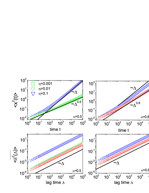
Figure 3: Top: Ensemble averaged MSD of the nCTRW process $x(t)$ with noise strengths $\eta=0.001$, $0.01$, and $0.1$, for anomalous diffusion exponents $\alpha=0.5$ (left) and $\alpha=0.8$ (right). A turnover from subdiffusive to Brownian (linear) scaling is observed. Bottom: trajectory-averaged time averaged MSD $\langle\overline{\delta^{2}(\Delta)}\rangle$ for $x(t)$ for the same values of $\eta$ and $\alpha$. The overall measurement time is $T=10^{5}$ in units of $\delta t$.

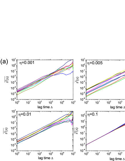
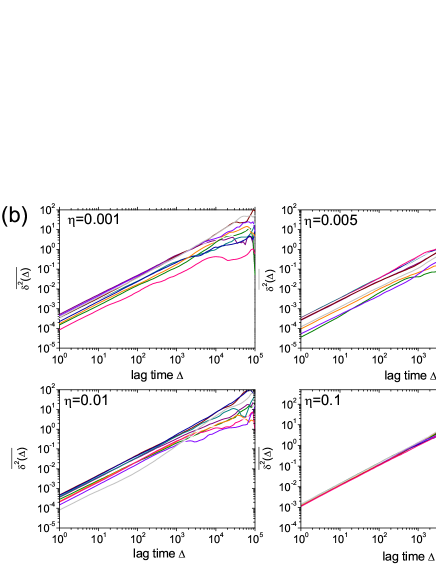
Figure 4: Ten individual time averaged MSD curves for nCTRW with (a) $\alpha=0.5$ and (b) $\alpha=0.8$ with added Brownian noise, for the same parameters as in Fig. 3. The relative amplitude scatter dramatically reduces at high noise strength.

From the simulated trajectories we evaluate the ensemble-averaged MSD for the nCTRW and study how its scaling behavior is affected by the Brownian noise $z_{B}(t)$. Fig. 3 summarizes the results for the nCTRW process with $\alpha=0.5$ and $\alpha=0.8$. In both cases, a common feature is that the ensemble averaged MSD exhibits a continuous transition from subdiffusion with anomalous diffusion exponent $\alpha$ to normal diffusion. This occurs either as the noise strength $\eta$ is increased at fixed time $t$, or as time $t$ is increased at a fixed $\eta$. Due to the additivity of the two contributions we obtain

$$\langle x^{2}(t)\rangle=\frac{2K_{\alpha}}{\Gamma(1+\alpha)}t^{\alpha}+2\eta^{2}Dt,$$ (19)

which is valid as long as $t$ is considerably larger than the time increment $\delta t$. Eq. (19) demonstrates that for the subdiffusive CTRW processes $x_{\alpha}(t)$ with $0<\alpha<1$ the ensemble averaged MSD of the nCTRW $x(t)$ has a crossover in its scaling from $\simeq t^{\alpha}$ at short times to $\simeq t$ at long times, with the crossover time scale $t_{c}\sim\left(K_{\alpha}/[\Gamma(1+\alpha)\eta^{2}D]\right)^{1/(1-\alpha)}$. That is, the effect of the Brownian noise $z_{B}(t)$ emerges only at long times $t>t_{c}$. Conversely, below $t_{c}$ the process appears to behave as the bare CTRW process. Note that the crossover time $t_{c}$ rapidly decreases with increasing $\eta$ as $t_{c}\sim\eta^{-2/(1-\alpha)}$. This explains why we only observe normal diffusion behavior without crossover for the largest noise strength $\eta=0.1$. The crossover time $t_{c}$ also rapidly increases as the exponent $\alpha$ approaches to one [as $K_{\alpha}\sim\Gamma(1-\alpha)$ in our choice of $\tau_{0}=1$, see Eq. (16)]. Accordingly, in Fig. 3 the ensemble averaged MSDs for $\alpha=0.8$ do not fully reach the linear regime within the time window of our simulation, in contrast to the case for $\alpha=0.5$ with $\eta=0.1$.

IV.2 Time-averaged mean squared displacement

We now consider the individual time averaged MSDs $\overline{\delta^{2}(\Delta)}$ of the nCTRW process from single trajectories $x(t)$ according to our definition in Eq. (3). Fig. 3 presents the trajectory-to-trajectory average (4). In all cases we find that the time averaged MSDs grow linearly with lag time $\Delta$ in the entire range of $\Delta$, showing a clear disparity from the scaling behavior of the ensemble averaged MSDs above. In the time averaged MSD the Brownian noise $z_{B}(t)$ simply affects the apparent diffusion constant, that is, the effective amplitude of the linear curves. To understand this phenomenon quantitatively, we obtain the analytical form of the trajectory-averaged time averaged MSD,

$$\left<\overline{\delta^{2}(\Delta)}\right>\sim\frac{2K_{\alpha}\Delta}{\Gamma(1+\alpha)T^{1-\alpha}}+2\eta^{2}D\Delta,$$ (20)

valid for $\Delta\ll T$. Eq. (20) shows that both contributions the naked CTRW $x_{\alpha}(t)$ and the Brownian process $\eta z_{B}(t)$ are linearly proportional to the lag time $\Delta$. Note that the exponent $\alpha$ and the noise strength $\eta$ only enter into the apparent diffusion constant

$$D_{\mathrm{app}}\equiv\frac{K_{\alpha}T^{\alpha-1}}{\Gamma(1+\alpha)}+\eta^{2}D,$$ (21)

where $\langle\overline{\delta^{2}(\Delta)}\rangle=2D_{\mathrm{app}}\Delta$. This result indicates that the effect of the Brownian noise cannot be noticed when we exclusively consider the scaling behavior of the time averaged MSD. Also in terms of the apparent diffusion constant, one hardly notices the presence of the Brownian noise component as long as $\eta$ is small. This agrees with our observations for the time averaged MSD curves in Fig. 3 for noise strengths $\eta=0.001$ and $0.01$.

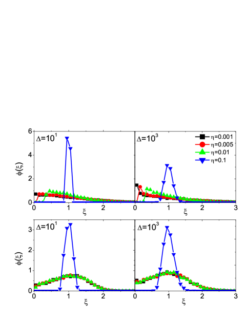
Figure 5: Variation of normalized scatter distributions $\phi(\xi)$ as a function of dimensionless variable $\xi=\overline{\delta^{2}}/\langle\overline{\delta^{2}}\rangle$ for the cases of $\eta=0.001$ (black square), 0.005 (red circle), 0.01 (green upper-triangle), and 0.1 (blue down-triangle). (Upper panels) $\alpha=0.5$. (Lower panels) $\alpha=0.8$. In each figure the results were obtained from $10^{4}$ runs.

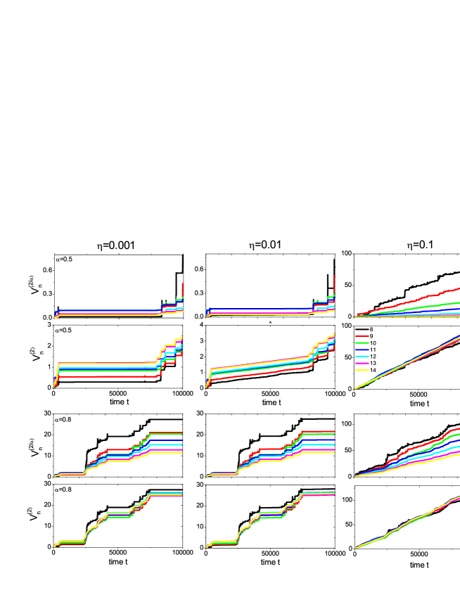
Figure 6: Results of the $p$-variation test for the nCTRW process with Brownian noise $\eta z_{B}(t)$ for noise strengths $\eta=0.001$, $\eta=0.01$, and $\eta=0.1$. The upper (lower) two rows are for $\alpha=0.5$ and $0.8$. In all figures the $p$ sums are plotted with the same color code: $n=8$ (black), 9 (red), 10 (green), 11 (blue), 12 (cyan), 13 (violet), and 14 (yellow).

We also check the fluctuations between individual time averaged MSD curves $\overline{\delta^{2}(\Delta)}$. Each panel in Fig. 4 plots ten individual time averaged MSDs for the nCTRW process. In all cases, the individual time averaged MSDs display linear scaling with lag time $\Delta$, namely, the scaling behavior of $\langle\overline{\delta^{2}(\Delta)}\rangle$. The individual amplitudes scatter, that is, the apparent diffusion constant $D_{\mathrm{app}}$ fluctuates. With increasing strength of the Brownian component the relative scatter between individual trajectories dramatically diminishes, leading to an apparently ergodic behavior. Thus, for the largest noise strength $\eta=0.1$, the ten trajectories almost fully collapse onto a single curve for $\Delta\ll T$.

IV.3 Scatter distribution

We quantify the amplitude scatter of the individual time averaged MSDs in terms of the normalized scatter distributions $\phi(\xi)$, where the dimensionless variable $\xi$ stands for the ratio $\xi=\overline{\delta^{2}}/\langle\overline{\delta^{2}}\rangle$ of individual traces $\overline{\delta^{2}}$ versus the trajectory average $\langle\overline{\delta^{2}}\rangle$ (compare the derivations in Refs. pt ; He ; stas2 ). Fig. 5 shows $\phi(\xi)$ for several values of the lag time $\Delta$. When the noise is negligible ($\eta=0.001$), the observed broad distribution is nearly that of the pure CTRW process. For $\alpha=1/2$ the distribution has the expected Gaussian profile centered at $\xi=0$ He , indicating that long stalling events of the order of the entire measurement time $T$ occur with appreciable probability. In the opposite case $\eta=0.1$, the Brownian noise results in a relatively sharply peaked, bell-shaped distribution typical for ergodic processes, at all lag times. An interesting effect of the Brownian noise is that at intermediate strengths it only tends to suppress the contribution at around zero while it does not significantly change the overall profile of the distribution compared to the noise-free case. This implicates that the trajectories share non-ergodic and ergodic elements. For instance, the trajectory of the nCTRW process $x(t)$ itself for $\eta=0.01$ in Fig. 2 shows a substantially blurred profile of the underlying CTRW process $x_{\alpha}(t)$ due to the relatively strong Brownian noise; however, the time averaged MSD and its distribution do exhibit non-ergodic behavior, as shown in Fig. 5. The case $\alpha=0.8$ shown in Fig. 5 features similar albeit less pronounced effects. In particular, $\phi(\xi)$ for the naked CTRW has its maximum at the ergodic value $\xi=1$. Again, the effect of the Brownian noise is to suppress the contribution at $\xi=0$.

IV.4 $p$-variation test

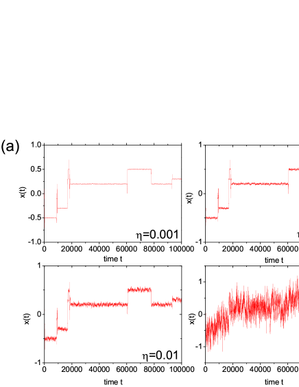
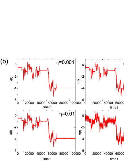
Figure 7: Sample trajectories of the nCTRW process $x(t)$ with Ornstein-Uhlenbeck noise for several values of the noise strength $\eta$ and anomalous diffusion exponents (a) $\alpha=0.5$ and (b) $\alpha=0.8$. In contrast to the Brownian noise case of Fig. 2, however, the approximately constant amplitude of the superimposed noise is characteristic for the Ornstein-Uhlenbeck process.

We now turn to the $p$-variation test and investigate its sensitivity to the additional noise in the nCTRW process, in comparison to the established results for the naked CTRW $x_{\alpha}(t)$. From the trajectory $x(t)$, the partial sum $V_{n}^{(p)}(t)$ is calculated for finite $n$ according to definition (5), where we choose $p=2/\alpha$ and $p=2$, compare Section II.2. In Fig. 6, we plot the results of the $p$-variation at increasing $n$ for the nCTRW process. We observe that for both cases $\alpha=0.5$ and $0.8$, the $p$-sums behave analogously to the predictions for the naked CTRW process, as long as the noise strength remains sufficiently small, according to Fig. 6 this holds for $\eta=0.001$ and 0.005 (not shown). In this case, $V_{n}^{(2/\alpha)}(t)$ monotonically decreases with increasing $n$, indicating the limiting behavior $V_{n}^{(2/\alpha)}(t)\rightarrow 0$ for large $n$. Meanwhile, $V_{n}^{(2)}(t)$ approaches the monotonic step-like behavior typical for the CTRW process $x_{\alpha}(t)$, as $n$ increases. Note that the $p$-sums have plateaus in their increments in analogy to the noise-free case due to the long stalling events in the trajectory.

As the magnitude of the Brownian noise grows larger ($\eta=0.01$ and 0.1), however, the behavior of the $p$-sums changes significantly. While $V_{n}^{(2/\alpha)}(t)$ decreases with increasing $n$ as for the weaker noise case, it increases linearly with $t$ nearly without any sign of plateaus for both nCTRW processes of $\alpha=0.5$ and 0.8 when the noise strength is increased to $\eta=0.1$. This new feature is the expected behavior of $V_{n}^{(p)}(t)$ with $p>2$ for a Brownian diffusive process (see Sec. II.2 and Fig. 1). Indeed, it can be shown that for $p=4$ the $p$-sum of the Brownian noise $z_{B}(t)$ behaves as $V_{n}^{(4)}(t)\sim(\frac{T}{2^{n}})t$. We note that for the Brownian noise $z_{B}(t)$ the $p$-sum $V_{n}^{(p)}(t)$ with $p>2$ always decays out to zero as $n\rightarrow\infty$. Therefore, the nCTRW process will always have the same $p$ variation result of $V_{n}^{(2/\alpha)}=0$ (in the limit of $n\rightarrow\infty$) as the pure CTRW $x_{\alpha}(t)$, even in case that its profile is dominated by large noise.

In contrast, the $p$-sum $V_{n}^{(2)}(t)$ exhibits a more distinguished effect of the Brownian noise due to the fact that the Brownian noise $\eta z_{B}(t)$ has $V_{n}^{(2)}(t)\simeq\eta^{2}2Dt$. Especially, we find that the noise effect is pronounced for the nCTRW with $\alpha=0.5$, when the underlying CTRW process $x_{\alpha}(t)$ features only few jumps. In this case, the Brownian noise of moderate strength ($\eta=0.01$) causes an incline with almost identical slope to the step-like profiles of $V_{n}^{(2)}(t)$. At the strongest noise $\eta=0.1$, the step-like behavior typical for the naked CTRW process $x_{\alpha}(t)$ is nearly masked and the overall tendency follows that of Brownian motion shown in Fig. 1. Accordingly, the $p$-variation test does not properly pin down the underlying CTRW process $x_{\alpha}(t)$ and thus potentially produces inconsistent conclusion for the nCTRW process. A qualitatively identical behavior is obtained for the nCTRW process when the underlying CTRW process $x_{\alpha}(t)$ performs relatively frequent jumps (corresponding to the case of $\alpha=0.8$). However, here the effect of the Brownian noise appears weak, because the contribution of $z_{B}(t)$ relative to the magnitude of $x_{\alpha}(t)$ becomes smaller at larger $\alpha$ values, see the trajectories $x(t)$ in Fig. 2.

V nCTRW with Ornstein-Uhlenbeck noise

We now turn to nCTRW processes $x(t)$, in which the superimposed noise is of Ornstein-Uhlenbeck form (18). In this case the influence of the added noise is expected to diminish as the process develops, according to our discussion in Sec. III.

Fig. 7 shows simulated trajectories for the nCTRW process $x_{\alpha}(t)$ with two different anomalous diffusion exponents, (a) $\alpha=0.5$ and (b) $\alpha=0.8$, for different noise strengths $\eta$. Indeed we observe that, compared to case of Brownian noise depicted in Fig. 2 the profiles of the jumps and rests of the naked CTRW motion $x_{\alpha}(t)$ are relatively well preserved despite the mixing with the Ornstein-Uhlenbeck noise $z_{OU}(t)$. Note that the simulated trajectories with moderate noise strength appear quite similar to the experimental traces of the microbeads in the reconstituted actin network reported by Wong et al. wong . The noise interference appears considerably lesser for the case $\alpha=0.8$, when the magnitude of the net displacements is large relative to the noise contribution due to frequent jumps in the trajectory $x_{\alpha}(t)$ when $\alpha$ is closer to unity. Only for the highest noise strength the pure CTRW behavior with its distinct sojourns becomes blurred by the Ornstein-Uhlenbeck noise.

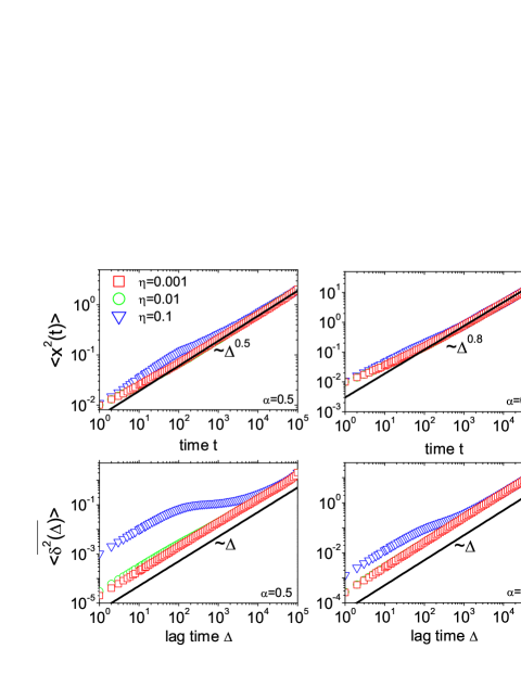
Figure 8: Top: Ensemble-averaged MSD $\langle x^{2}(t)\rangle$ of the nCTRW process with Ornstein-Uhlenbeck noise for anomalous diffusion exponents $\alpha=0.5$ and $0.8$. Bottom: Trajectory-average of the time averaged MSD $\langle\overline{\delta^{2}(\Delta)}\rangle$ for the same $\alpha$. We use $T=10^{5}$.

V.1 Ensemble-averaged mean squared displacement

In Fig. 8 we plot the ensemble averaged MSD $\langle x^{2}(t)\rangle$ of the nCTRW process with Ornstein-Uhlenbeck noise for different noise strengths $\eta$. We note that, regardless of the intensity $\eta$, the ensemble averaged MSDs follow the scaling law $\sim t^{\alpha}$ of the noise-free CTRW process $x_{\alpha}(t)$, in particular, at long times. Moreover, all MSD curves at different $\eta$ almost collapse onto each other, although small differences are discernible at short times. These results suggest that, in contrast to the Brownian noise case discussed in Sec. IV, the Ornstein-Uhlenbeck noise does not critically interfere with the diffusive behavior of the noise-free CTRW motion, as expected. To obtain a quantitative understanding of these results we derive the analytic form of the ensemble averaged MSD,

$$\langle x^{2}(t)\rangle=\frac{2K_{\alpha}}{\Gamma(1+\alpha)}t^{\alpha}+\frac{\eta^{2}D}{k}\left(1-e^{-2kt}\right).$$ (22)

Here the last term stems from the contribution of the Ornstein-Uhlenbeck noise. For $t>k^{-1}$ it saturates to the constant $\eta^{2}D/k$, which is typically small relative to $2K_{\alpha}t^{\alpha}/\Gamma(1+\alpha)$. Hence, at long times $t>k^{-1}$, the noise term is negligible, and the ensemble averaged MSD grows as $2K_{\alpha}t^{\alpha}/\Gamma(1+\alpha)$, consistent with the observations in Fig. 8. In the opposite case for $t<k^{-1}$, the contribution of the noise is expanded to obtain $\langle z_{OU}^{2}(t)\rangle\approx 2\eta^{2}Dt$. As discussed for the characteristic function (14), on these time scales the Ornstein-Uhlenbeck noise $z_{OU}(t)$ has the same form as the Brownian noise $z_{B}(t)$, leading to the same scaling form (19) for the ensemble averaged MSD. However, as studied in the previous case, the effect of the linear scaling is irrelevant at short times.

V.2 Time-averaged mean squared displacement

We now turn to the time averaged MSD curves $\overline{\delta^{2}(\Delta)}$ from individual trajectories $x(t)$ of the nCTRW process. Fig. 8 shows the trajectory-averaged time averaged MSD $\langle\overline{\delta^{2}(\Delta)}\rangle$ for different noise strengths. For both anomalous diffusion exponents $\alpha=0.5$ and $0.8$, we observe qualitatively the same behavior. On the one hand, the CTRW motion superimposed with moderate noise ($\eta=0.001$ and $0.01$) leads to a linear scaling of the time averaged MSD with lag time $\Delta$, with almost identical amplitude. On the other hand, when the noise amplitude becomes large, the scaling of the time averaged MSD is significantly affected. We find that these results are consistent with the analytical form of the trajectory-averaged time averaged MSD,

$$\left<\overline{\delta^{2}(\Delta)}\right>\sim\frac{2K_{\alpha}\Delta}{\Gamma(1+\alpha)T^{1-\alpha}}+\frac{2\eta^{2}D}{k}\left(1-e^{-k\Delta}\right),$$ (23)

valid at lag times $\Delta\ll T$. In this expression it is worthwhile to point out that the contribution of the naked CTRW process $x_{\alpha}(t)$ is decreased as the length of the trajectory becomes longer, due to the aging effect of the decreasing effective diffusion constant $\simeq T^{\alpha-1}$, while the noise is independent of $T$. Due to this effect the time averaged MSD (23) has three distinct scaling regimes: (i) at lag times $\Delta\gg k^{-1}$, the time averaged MSD is linearly proportional to the lag time with apparent diffusion constant $D_{\mathrm{app}}\approx K_{\alpha}T^{\alpha-1}/\Gamma(1+\alpha)$. (ii) At lag times $\Delta\ll k^{-1}$, the time averaged MSD is again proportional to $\Delta$. On this timescale, however, the noise part cannot be ignored, and the apparent diffusion constant is given by $D_{\mathrm{app}}\approx K_{\alpha}T^{\alpha-1}/\Gamma(1+\alpha)+\eta^{2}D$. Note that the diffusion constant at short lag times is larger than the one at long times. (iii) For lag times $\Delta\approx k^{-1}$, the time averaged MSD is that of confined Brownian diffusion where $\langle\overline{\delta^{2}(\Delta)}\rangle\approx 2K_{\alpha}T^{\alpha-1}\Delta/\Gamma(1+\alpha)+2\eta^{2}D$. These three regimes are expected to occur only in the presence of large noise strengths when $\eta^{2}D>K_{\alpha}T^{\alpha-1}/\Gamma(1+\alpha)$ (see the case $\eta=0.1$ in Fig. 8). In the opposite case, when $2\eta^{2}D$ is negligible compared to $K_{\alpha}T^{\alpha-1}/\Gamma(1+\alpha)$, the three regimes are indistinguishable, and only one scaling law $\langle\overline{\delta^{2}(\Delta)}\rangle\approx 2K_{\alpha}T^{\alpha-1}\Delta/\Gamma(1+\alpha)$ is observed at all lag times. This behavior is seen for the two cases of $\eta=0.001$ and $0.01$ in Fig. 8.

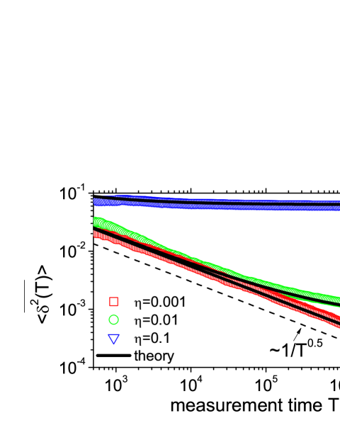
Figure 9: Profiles of the time averaged MSD $\langle\overline{\delta^{2}(\Delta,T)}\rangle$ as a function of measurement time $T$ at a fixed lag time $\Delta=100$. We show the nCTRW of $\alpha=0.5$ with $\eta z_{OU}(t)$ at $\eta=0.001$, 0.01, and 0.1 (from bottom to top). Solid and dotted lines represent the analytical form (23) and the scaling $\sim T^{\alpha-1}$, respectively.

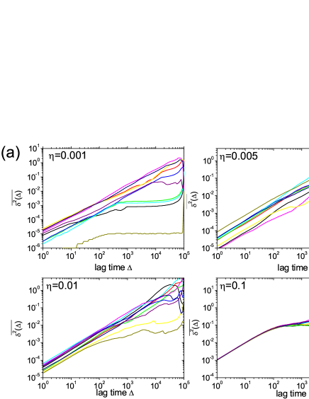
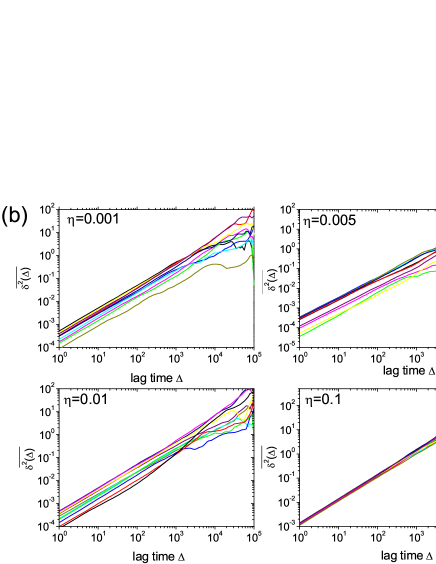
Figure 10: Ten individual time averaged MSD curves of the nCTRW process with Ornstein-Uhlenbeck noise of strengths $\eta=0.001$, $0.005$, $0.01$, and $0.1$ for anomalous diffusion exponents (a) $\alpha=0.5$ and (b) $\alpha=0.8$. $T=10^{5}$ is used as in Fig. 8.

Interestingly, the time averaged MSD for the nCTRW with anomalous diffusion exponent $\alpha=0.5$ and noise strength $\eta=0.1$ is reminiscent of the MSD curves observed for micron-sized tracer particles immersed in wormlike micellar solutions, which are known to behave as a viscoelastic polymer network when the micelles concentration is above a critical value dreiss . Experiments using diffusing wave spectroscopy galvan ; bellour and single-particle tracking natascha1 revealed that the immersed particles exhibit three distinct diffusive behaviors in different time windows. It was shown that particles surrounded by the micellar network undergo a Brownian diffusion at short (sub-milliseconds) times until they engage with the caging effects of the micellar network, while at later times (milliseconds to sub-seconds) one observes a seemingly confined Brownian motion. It turns out that this confined diffusion is in fact a pronounced subdiffusive motion characterized by anti-persistent spatial correlation induced by the polymer network, governed by the fractional Langevin equation natascha1 . At macroscopic times, when the wormlike micelle solution behaves as a viscous fluid, the particle again shows a Brownian diffusion, albeit with a significantly reduced diffusion constant. The results obtained here suggest that due to the presence of the Ornstein-Uhlenbeck noise the CTRW process could be mistakenly interpreted to conform to a physically different system, i.e., Brownian motion, and, thus, one needs to be careful in analyzing the data with several possible models, and to use several complementary diagnosis tools.

The expression (23) for the time averaged MSD suggests that $\overline{\delta^{2}(\Delta,T)}$ stops aging and reflects almost entirely the character of the Ornstein-Uhlenbeck noise process if $T\gtrsim T_{\mathrm{cr}}\sim(kK_{\alpha}\Delta/[\Gamma(1+\alpha)\eta^{2}D])^{1/(1-\alpha)}$. This is indeed shown in Fig. 9 where the time averaged MSD $\langle\overline{\delta^{2}(\Delta,T)}\rangle$ is plotted as a function of the overall measurement time $T$ at a fixed lag time $\Delta=100$ for nCTRW with $\alpha=0.5$, together with the theoretical prediction Eq. (23). For the weakest noise $\eta=0.001$ whose crossover time $T_{\mathrm{cr}}\sim 10^{9}$ is beyond $T_{\mathrm{max}}=10^{7}$, the time averaged MSD only displays aging of the naked CTRW process with scaling $\sim T^{\alpha-1}$. When the noise strength is increased to $\eta=0.01$, the time averaged MSD starts to show ergodic behavior as the measurement time $T$ gets larger than the crossover time $T_{\mathrm{cr}}\sim 10^{5}$. In the extreme case when the nCTRW process is dominated by the noise (here $\eta=0.1$), effectively no aging is observed in $\overline{\delta^{2}(\Delta,T)}$ and the process appears ergodic.

In Fig. 10 we plot ten individual time averaged MSD curves $\overline{\delta^{2}(\Delta)}$. For the case of more pronounced subdiffusion ($\alpha=0.5$), the trajectory-to-trajectory variations are significant, due to the combined effect of long-time stalling events and the Ornstein-Uhlenbeck noise. Thus, for the smallest noise strength $\eta=0.001$ some time averaged MSDs exhibit a large deviation from the linear scaling $\sim\Delta$ expected from the trajectory-averaged time averaged MSD. In this case, the long stalling events, that are of the order of the measurement time $T$, lead to the plateaus in $\overline{\delta^{2}(\Delta)}$. Intriguingly, such plateaus also appear in the presence of the largest noise strength, $\eta=0.1$. Here, however, they represent the confined diffusion of the Ornstein-Uhlenbeck noise in which one or few long-stalling events occur in the the CTRW process. For the CTRW process with more frequent jumps ($\alpha=0.8$) the individual time averaged MSDs follow the expected scaling behavior with smaller amplitude fluctuations in $\overline{\delta^{2}(\Delta)}$, as now the noise is relatively stronger.

V.3 Scatter distribution

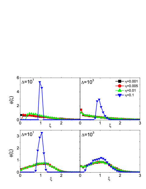
Figure 11: Normalized scatter distribution $\phi(\xi)$ as a function of the dimensionless variable $\xi=\overline{\delta^{2}}/\langle\overline{\delta^{2}}\rangle$ for the cases of $\eta=0.001$ (black square), 0.005 (red circle), 0.01 (green upper-triangle), and 0.1 (blue down-triangle). Top: $\alpha=0.5$. Bottom: $\alpha=0.8$. In each panel the results were obtained from $10^{4}$ runs.

Fig. 11 illustrates the normalized scatter distribution $\phi(\xi)$ of the individual time averaged MSDs obtained from $10^{4}$ trajectories, as a function of the dimensionless variable $\xi=\overline{\delta^{2}}/\langle\overline{\delta^{2}}\rangle$. The overall behavior is qualitatively consistent with those of the scatter distributions for added Brownian noise, as shown in Fig. 5. The distribution becomes increasingly ergodic as the Gaussian noise increases, especially for the case of the more pronounced subdiffusive process ($\alpha=0.5$). Here, the finite contribution at $\xi=0$ in $\phi(\xi)$ is gradually suppressed and the peak of the distributions is approaching $\xi=1$ as the strength of the noise is increased.

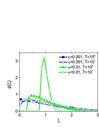
Figure 12: Dependence of the overall measurement time $T$ on the normalized scatter distribution $\phi(\xi)$. The distributions obtained from the nCTRW process with $T=10^{7}$ are compared to the distributions from the one with $T=10^{5}$. Results from nCTRW process of anomalous exponent $\alpha=0.5$ mixed with $\eta z_{OU}(t)$ at $\eta=0.001$ and 0.01.

From the time averaged MSD (23) and its aging property in Fig. 9 it is also expected that the distribution attains apparent ergodic features as the observation time $T$ is increased. We show this in Fig. 12 where the scatter distributions for the same nCTRW process simulated up to $T=10^{7}$ are compared to the previous ones with $T=10^{5}$. The general trend is that $\phi(\xi)$ becomes sharper as $T$ increases. Importantly, this ergodic effect becomes relevant provided that $T$ is increased to at least be comparable with the crossover time $T_{\mathrm{cr}}\sim(kK_{\alpha}\Delta/[\Gamma(1+\alpha)\eta^{2}D])^{1/(1-\alpha)}$ defined above. As seen for the case for $\eta=0.001$, the distribution $\phi(\xi)$ is almost unaffected, except at $\xi\approx 0$ where $T\ll T_{\mathrm{cr}}(\sim 10^{9})$. In contrast to this, the distribution at $\eta=0.01$ is noticeably narrower around $\xi=1$ when $T$ is increased ($T_{\mathrm{cr}}\sim 10^{5}$).

V.4 $p$-variation test

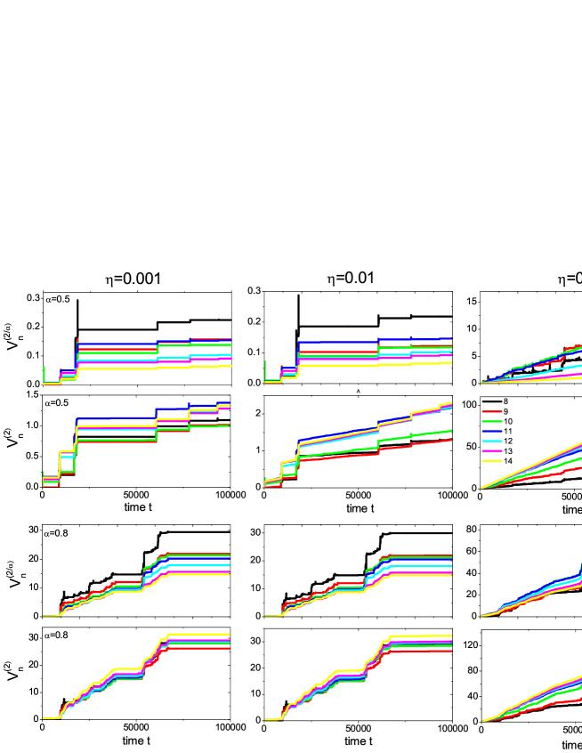
Figure 13: Results of the $p$-variation test for nCTRW with superimposed Ornstein-Uhlenbeck noise $\eta z_{OU}(t)$ for noise strengths $\eta=0.001$, $\eta=0.01$, and $\eta=0.1$. The upper and lower two rows are for $\alpha=0.5$ and $0.8$. Same color codes as those of Fig. 6.

In Fig. 13 we show the variation of the $p$-sums $V_{n}^{(2/\alpha)}(t)$ and $V_{n}^{(2)}(t)$ at increasing $n$ for the simulated trajectories $x(t)$ of Fig. 7. For the smallest noise strength $\eta=0.001$ shown in Fig. 13 the $p$-variation test produces the result expected for the naked CTRW process. In the case of nCTRW with $\alpha=0.8$ this behavior persists in the presence of large noise strengths up to $\eta=0.01$. This is due to the fact that the naked CTRW process $x_{\alpha}(t)$ features large displacements relative to those of the Ornstein-Uhlenbeck process. In contrast, for $\alpha=0.5$ the profiles of $V_{n}^{(2)}(t)$ are mildly affected by the Ornstein-Uhlenbeck noise. Namely, the plateaus are tilted, with a somewhat larger slope at higher $\eta$, while their overall profiles preserve features of the monotonic, step-like behavior of the CTRW process $x_{\alpha}(t)$.

Concurrently, we note that at larger values of $\eta$ neither $V_{n}^{(2)}(t)$ nor $V_{n}^{(2/\alpha)}(t)$ show any indication of CTRW for both $\alpha=0.5$ and $0.8$. At these noise strengths, the Ornstein-Uhlenbeck noise dominates the $p$-variation results. As explained in Section II.2 and shown in Fig. 1, in the limit $n\rightarrow\infty$ the $p$-sums for the Ornstein-Uhlenbeck noise converge to the results for Brownian noise. Thus, while $V_{n}^{(2/\alpha)}(t)$ rapidly decreases with increasing $n$ in the case of Brownian noise, such a tendency is also present for the Ornstein-Uhlenbeck noise. Moreover, the spike-like profiles in $V_{n}^{(4)}(t)$ at $n=8$ for $\eta=0.1$ reflects the property of the Ornstein-Uhlenbeck noise (see Fig. 1). For $p=2$, we find that the $p$-sum of the Ornstein-Uhlenbeck noise$z_{OU}(t)$ behaves as $V_{n}^{(2)}(t)\sim\frac{2D}{k}\left[1-\exp(-\frac{k}{2}\frac{T}{2^{n}})\right]\left(\frac{2^{n}}{T}\right)t$ (see App. A). This result explains why $V_{n}^{(2)}(t)$ monotonically increases with $n$ up to $n\sim\log(kT)/\log 2\approx 10$, and for $n$ larger it grows as $V_{n}^{(2)}(t)\sim 2Dt$, as shown in Fig. 13. As in the case of the above nCTRW in the presence of Brownian noise $z_{B}(t)$, we find that the $p$-variation result may be substantially affected by the added Ornstein-Uhlenbeck noise, and the identification of the underlying CTRW process become impossible.

VI Conclusions

We introduced the noisy CTRW process, in which an ordinary CTRW process is superimposed with Gaussian noise, representing physically relevant cases when the pure CTRW motion becomes distorted by a noisy environment. We investigated how the additional ergodic noise interferes with the non-ergodic behaviors of the underlying subdiffusive CTRW motion. Considering the two types of Gaussian noise, Brownian noise and Ornstein-Uhlenbeck noise, we simulated the resulting nCTRW motion and studied physical quantities such as the ensemble and time averaged MSDs, the amplitude scatter distribution, and the behavior of the $p$-variation.

The analysis demonstrates that the influence of the Gaussian noise on these statistical quantities is highly specific to the quantity of concern. Moreover, it depends not only on the type of the noise and its strength but also on the length of the trajectory and the time scale. Depending on those specific conditions a quantitative analysis of the nCTRW process may reveal or mask the underlying non-ergodicity of the naked CTRW process. Thus care is needed when we want to diagnose the stochastic nature of a physical process based on experimental data. One way to avoid wrong conclusions is to apply complementary analysis techniques, such as the quantities used herein, or moment ratios, mean maximal excursion methods, first passage dynamics, or others. The other necessary ingredient is a good physical intuition for the observed process. It would be also interesting to find analytical expressions for the $p$-variations, of mixed processes, as those we have considered here. Our simulations results show that on finite measurement time the noise is crucial, and could easily destroy our basic understanding of the underlying process.

From the present study an experimentally relevant inverse problem can be posed. Can one filter out the Gaussian noise from the experimentally obtained nCTRW process? Although obtaining the noise-cleansed profile from a given nCTRW trajectory may appear infeasible, one could in principle obtain noise-free contribution in some ensemble- or time-averaged physical quantities of the nCTRW process provided one is able to attain a sufficiently long trajectory. In the ensemble averaged MSD the noise survives if the noise is Brownian motion while the CTRW process wins if the noise is of Ornstein-Uhlenbeck type [see Eq. (22)]. This is of course what we expect, since the MSD of the Brownian motion increases linearly with time, for CTRW like $t^{\alpha}$, and is a constant for Ornstein-Uhlenbeck—hence it is not surprising to see this behavior. In contrast for the time averaged MSD the dominant contribution comes always from the noise [Eqs. (20) and (23)] in the sense that when the measurement time $T$ is very large even the bounded Ornstein-Uhlenbeck noise wins over. This is due to an aging effect, the time averaged MSD of the CTRW process decreases with measurement time $T$. We thus see that the influence of the noise on time averages is fundamentally different from that on ensemble averages. As an example, one can extract almost solely the noise contribution in the time-averaged MSD (and not the bare CTRW itself) from a very long nCTRW trajectory. For an ergodic process this corresponds to the almost identical noise contribution in the ensemble-averaged MSD, namely, $\eta^{2}\langle z^{2}(\Delta)\rangle\simeq\langle\overline{\delta^{2}(\Delta,T\rightarrow\infty)}\rangle$. How to subtract this noise from real data is left for future work.

The nCTRW process developed herein is a physical extension of pure CTRW dynamics. We believe that it represents an important advance in the truthful description of anomalous diffusion data in thermal microscopic systems, where the environment is noisy by definition. Mathematically, the nCTRW process is quite intuitive, due to the additivity of the Gaussian noise.

Our present study can naturally be extended to more complicated noise sources, such as fractional Brownian motion (FBM), in order to obtain insight into intracellular anomalous diffusion that show both CTRW and FBM behaviors. It is expected that although FBM-like noise should lead to similar effects on the statistical behavior of the nCTRW process, the quantitative results will be profoundly different due to the scaling law of the FBM-like noise $\langle z_{\mathrm{FBM}}^{2}(t)\rangle\sim t^{\alpha^{\prime}}$ with exponent $0<\alpha^{\prime}<2$.

Appendix A $p$-variation of CTRW subdiffusion and Ornstein-Uhlenbeck noise

We here discuss the $p$-variation properties of CTRW subdiffusion and the Ornstein-Uhlenbeck noise in some more detail.

CTRW subdiffusion. The subdiffusive CTRW process $x_{\alpha}(t)$ with its PDF governed by the fractional Fokker-Planck equation (8) can be described through the subordinated Brownian motion $x_{\alpha}(t)=B(S_{\alpha}(t))$, where $B(\tau)$ defined with the internal time $\tau$ is an ordinary Brownian motion satisfying $\langle B(\tau)\rangle=0$ and $\langle B^{2}(\tau)\rangle=2D\tau$. Here, $S_{\alpha}(t)$ is the so called inverse subordinator matching the laboratory time $t$ to the internal time $\tau$. For the CTRW process $x_{\alpha}(t)$, the $p$-sum $V_{n}^{(2)}$(t) as $n$ grows to infinity satisfies marcin

$$V^{(2)}(t)=2DS_{\alpha}(t).$$ (24)

As shown in Fig. 1, $S_{\alpha}(t)$ has a step-like incremental profile and its jump times represent those for a given realization of CTRW process $x_{\alpha}(t)$. On the other hand, the $p$-sum $V_{n}^{(2/\alpha)}(t)$ (with $0<\alpha<1$) decreases with increasing $n$, finally $V^{(2/\alpha)}(t)=0$ at $n\rightarrow\infty$ marcin . This is also shown in the simulations in Fig. 1.

Ornstein-Uhlenbeck noise. The ensemble average of the $p$-variation sum at finite $n$ becomes

$$\left<V_{n}^{(2)}(t)\right>\approx\frac{2D}{k}\left[1-\exp\left(-\frac{k}{2}\frac{T}{2^{n}}\right)\right]\left(\frac{2^{n}}{T}\right)t,$$ (25)

neglecting an additional term which becomes negligible for large $T$. For small $n\lesssim\log(kT)/\log 2$, the above $p$ sum simplifies to

$$\langle V_{n}^{(2)}(t)\rangle\approx\frac{2D}{k}\frac{2^{n}}{T}t.$$ (26)

In this case the linear slope of $\langle V^{(2)}(t)\rangle$ increased with $n$ up to values $\log(kT)/\log 2\sim 10$ (for the given parameter values used in our simulation). This is shown in Fig. 1. In the other case, when $n\rightarrow\infty$, the $p$ sum converges to the result of the Brownian noise $\langle V^{(2)}(t)\rangle\approx 2Dt$. Hence, for large $n\gtrsim\log(kT)/\log 2$, $\langle V^{(2)}(t)\rangle$ is proportional to $t$ with an $n$-independent slope. From the fact that on short-time scales (as $n\to\infty$) the Ornstein-Uhlenbeck process behaves like a free Brownian process, it can be inferred that its $p$-variation results are identical with those for simple Brownian motion. Therefore, $V^{(4)}(t)$ is expected to converge to zero as $n$ increases. This is indeed observed in the simulations result in Fig. 1. We find that when $n$ is small, the increment of $V^{(4)}(t)$ exhibits a spike-like profile. This behavior presumably occurs due to the fact that the quartic moment of the displacement $x((j+1)T/[2^{n}])-x(jT/[2^{n}])$ becomes very small when the lag time $T/2^{n}$ is larger than the relaxation time $1/k$ of the process for small $n$.

References

- (1) I. Y. Wong, M. L. Gardel, D. R. Reichman, E. R. Weeks, M. T. Valentine, A. R. Bausch, and D. A. Weitz, Phys. Rev. Lett. 92, 178101 (2004).
- (2) A. V. Weigel, B. Simon, M. M. Tamkun, and D. Krapf, Proc. Nat. Acad. Sci. USA 108, 6438 (2011).
- (3) S. M. A. Tabei, S. Burov, H. Y. Kim, A. Kuznetsov, T. Huynh, J. Jureller, L. H. Philipson, A. R. Dinner, and N. F. Scherer, Proc. Natl. Acad. Sci. USA 110, 4911 (2013).
- (4) J.-H. Jeon, V. Tejedor, S. Burov, E. Barkai, C. Selhuber-Unkel, K. Berg-Sørensen, L. Oddershede, and R. Metzler, Phys. Rev. Lett. 106, 048103 (2011).
- (5) E. Barkai, Y. Garini, and R. Metzler, Physics Today 65(8), 29 (2012).
- (6) S. Havlin and D. Ben-Avraham, Adv. Phys. 36, 695 (1987).
- (7) J.-P. Bouchaud and A. Georges, Phys. Rep. 195, 127 (1990).
- (8) R. Metzler and J. Klafter, Phys. Rep. 339, 1 (2000).
- (9) R. Metzler and J. Klafter, J. Phys. A 37, R161 (2004).
- (10) I. Golding and E. C. Cox, Phys. Rev. Lett. 96 098102 (2006).
- (11) F. Höfling and T. Franosch, Rep. Prog. Phys. 76, 046602 (2013).
- (12) M. J. Saxton and K. Jacobson, Annu. Rev. Biophys. Biomol. Struct. 26, 373 (1997).
- (13) H. Scher and E. W. Montroll, Phys. Rev. B 12, 2455 (1975).
- (14) H. Scher, G. Margolin, R. Metzler, J. Klafter, and B. Berkowitz, Geophys. Res. Lett. 29, 1061 (2002).
- (15) E. W. Montroll and G. H. Weiss, J. Math. Phys. 6, 167 (1965).
- (16) N. Leijnse, J.-H. Jeon, S. Loft, R. Metzler, and L. B. Oddershede, Eur. Phys. J. Special Topics 204, 75 (2012).
- (17) B. Berkowitz, A. Cortis, M. Dentz, and H. Scher, Rev. Geophys. 44, RG2003 (2006).
- (18) C. Monthus and J.-P. Bouchaud, J. Phys. A 29, 3847 (1996).
- (19) S. Burov and E. Barkai, Phys. Rev. Lett. 98, 250601 (2007).
- (20) R. Metzler, E. Barkai, and J. Klafter, Phys. Rev. Lett. 82, 3563 (1999); Europhys. Lett. 46, 431 (1999); E. Barkai, R. Metzler, and J. Klafter, Phys. Rev. E 61, 132 (2000).
- (21) I. Nordlund, Z. Phys. Chem. 87, 40 (1914).
- (22) C. Bräuchle, D. C. Lamb, and J. Michaelis, Single Particle Tracking and Single Molecule Energy Transfer (Wiley-VCH, Weinheim, Germany, 2012); X. S. Xie, P. J. Choi, G.-W. Li, N. K. Lee, and G. Lia, Annu. Rev. Biophys. 37, 417 (2008).
- (23) I. Bronstein, Y. Israel, E. Kepten, S. Mai, Y. Shav-Tal, E. Barkai, and Y. Garini, Phys. Rev. Lett. 103, 018102 (2009).
- (24) J. Szymanski and M. Weiss, Phys. Rev. Lett. 103, 038102 (2009).
- (25) J.-H. Jeon, N. Leijnse, L. B. Oddershede, and R. Metzler, New J. Phys. 15, 045011 (2013).
- (26) A. Caspi, R. Granek and M. Elbaum, Phys. Rev. Lett. 85, 5655 (2000).
- (27) D. Banks and C. Fradin, Biophys. J. 89, 2960 (2005).
- (28) S. C. Weber, A. J. Spakowitz, and J. A. Theriot, Phys. Rev. Lett. 104, 238102 (2010).
- (29) S. Burov, J.-H. Jeon, R. Metzler, and E. Barkai, Phys. Chem. Chem. Phys. 13, 1800 (2011).
- (30) Y. Meroz, I. Eliazar, and J. Klafter, J. Phys. A 42, 434012 (2009); Y. Meroz, I. M. Sokolov, and J. Klafter, Phys. Rev. Lett. 110, 090601 (2013).
- (31) W. Deng and E. Barkai, Phys. Rev. E 79, 011112 (2009).
- (32) J.-H. Jeon and R. Metzler, Phys. Rev. E 81, 021103 (2010). Note, however, the occurrence of transient non-ergodic relaxation to equilibrium under confinement, as shown in J.-H. Jeon and R. Metzler, Phys. Rev. E 85, 021147 (2012).
- (33) I. Goychuk, Phys. Rev. E 80, 046125 (2009); Adv. Chem. Phys. 150, 187 (2012).
- (34) G. R. Kneller, K. Baczynski, and M. Pasenkiewicz-Gierula, J. Chem. Phys. 135, 141105 (2011).
- (35) J.-H. Jeon, H. Martinez-Seara Monne, M. Javanainen, and R. Metzler, Phys. Rev. Lett. 109, 188103 (2012).
- (36) G. Zumofen and J. Klafter, Physica D 69, 436 (1993).
- (37) A. Godec and R. Metzler, Phys. Rev. Lett. 110, 020603 (2013).
- (38) D. Froemberg and E. Barkai, Phys. Rev. E. Rapid Com. 87, 031104(R) (2013).
- (39) J.-P. Bouchaud, J. Phys. I (Paris) 2, 1705 (1992).
- (40) G. Bel and E. Barkai, Phys. Rev. Lett. 94, 240602; A. Rebenshtok and E. Barkai, ibid. 99, 210601 (2007); J. Stat. Phys. 133, 565 (2008).
- (41) M. A. Lomholt, I. M. Zaid, and R. Metzler, Phys. Rev. Lett. 98, 200603 (2007); I. M. Zaid, M. A. Lomholt, and R. Metzler, Biophys. J. 97, 710 (2009).
- (42) Y. He, S. Burov, R. Metzler, and E. Barkai, Phys. Rev. Lett. 101, 058101 (2008).
- (43) A. Lubelski, I. M. Sokolov, and J. Klafter, Phys. Rev. Lett. 100, 250602 (2008).
- (44) J. H. P. Schulz, E. Barkai, and R. Metzler, Phys. Rev. Lett. 110, 020602 (2013); E. Barkai, ibid. 90, 104101 (2003); E. Barkai and Y-C. Cheng, J. Chem. Phys. 118, 6167 (2003).
- (45) S. Burov, R. Metzler, and E. Barkai, Proc. Natl. Acad. Sci. USA 107, 13228 (2010).
- (46) T. Neusius, I. M. Sokolov, and J. C. Smith, Phys. Rev. E 80, 011109 (2009).
- (47) I. M. Sokolov, E. Heinsalu, P. Hänggi and I. Goychuk, Europhys. Lett. 86, 30009 (2009).
- (48) M. J. Saxton, Biophys. J. 72, 1744 (1997).
- (49) A. Caspi, R. Granek, and M. Elbaum, Phys. Rev. E 66m 011916 (2002).
- (50) T. Akimoto, Phys. Rev. Lett. 108, 164101 (2012).
- (51) S. Condamin, V. Tejedor, R. Voituriez, O. Bénichou, and J. Klafter, Proc. Natl. Acad. Sci. USA 105, 5675 (2008).
- (52) V. Tejedor, O. Bénichou, R. Voituriez, R. Jungmann, F. Simmel, C. Selhuber-Unkel, L. Oddershede, and R. Metzler, Biophys. J. 98, 1364 (2010).
- (53) M. Bauer, R. Valiullin, G. Radons, and J. Kaerger, J. Chem. Phys. 135, 144118 (2011).
- (54) M. Magdziarz, A. Weron, K. Burnecki, and J. Klafter, Phys. Rev. Lett. 103, 180602 (2009); M. Magdziarz and J. Klafter, Phys. Rev. E 82, 011129 (2010).
- (55) K. Burnecki, E. Kepten, J. Janczura, I. Bronshtein, Y. Garini, and A. Weron, Biophys. J. 103, 1839 (2012).
- (56) I.M. Sokolov, E. Heinsalu, P. Hänggi, and I. Goychuk, EPL 86, 30009 (2009).
- (57) J.-H. Jeon and R. Metzler, J. Phys. A: Math. Theor. 43, 252001 (2010).
- (58) E. Barkai, R. Metzler, and J. Klafter, Phys. Rev. E. 61, 132 (2000). Note the occurrence of the factor here due to the different choice of in Eq. (15).
- (59) C. A. Dreiss, Soft Matter 3, 956 (2007).
- (60) J. Galvan-Miyoshi, J. Delgado, R. Castillo, Eur. Phys. J. E 26, 369 (2008).
- (61) M. Bellour, M. Skouri, J.-P. Munch, and P. Hébraud, Eur. Phys. J. E 8, 431 (2002).