Persistent current induced by vacuum fluctuations in a quantum ring

Abstract

We study theoretically interaction between electrons in a quantum ring embedded in a microcavity and vacuum fluctuations of electromagnetic field in the cavity. It is shown that the vacuum fluctuations can split electron states of the ring with opposite angular momenta. As a consequence, the ground state of electron system in the quantum ring can be associated to nonzero electric current. Since a ground-state current flows without dissipation, such a quantum ring gets a magnetic moment and can be treated as an artificial spin.

I Introduction

The interaction between light and matter represents an important part of the modern physics, from both fundamental and applied point of view. In particular, the vast fundamental research is devoted to studies of electromagnetic vacuum.Milonni Being one of the cornerstones of quantum electrodynamics, observing alteration of atom levels due to vacuum fluctuations (the Lamb shift) Lamb_47 ; Bethe_47 ; Scully_10 and attraction between conducting plates caused by radiational pressure of virtual photons (the Casimir effect) Casimir ; Fialkovsky_11 ; Sernelius_11 have led to deeper understanding of the electromagnetic field. However, the influence of vacuum fluctuations is usually minor in the non-relativistic physics and is only accessible in state-of-the-art experiments. Thus, the question of proposal for macroscopically observable effects caused by electromagnetic fluctuations of vacuum is still open.Jaffe

The physics of light-matter interaction contains the wide range of topics, namely cavity quantum electrodynamics,Dutra ; Review_CQED laser physics,LaserRev1 ; LaserRev2 polaritonics,KavokinBook ; PolaritonDevices etc. While most of the topics assume the emission and absorption of real photons by particles in a solid, the light-matter interaction is not only restricted to this case. For instance, the electronic states can be “dressed” by photons, changing the energy spectrum of electron-photon system, while photon absorption is prohibited.Cohen-Tannoudji_b98 This is the essence of dynamic Stark effect Autler studied before for various systems (see, e.g., Refs. [ScullyZubairy, ; Koch, ; Faist, ; Wu, ; Kibis_10, ; Vidar, ; Snoke, ]). However, previously proposed experimental configurations require the source of real photons which are directly detectable quanta of electromagnetic field. In this paper we study the dynamic Stark effect induced by virtual photons — vacuum fluctuations of electromagnetic field confined in a resonator — for the particular case of electron states in a quantum ring embedded in the optically chiral resonator. Due to the vacuum-induced splitting of electron energy levels with opposite angular momenta, the ground state of electron system in the ring can be associated to nonzero angular momentum. As a consequence, a ground-state dissipationless electric current (persistent current) appears. It should be stressed that the discussed phenomenon differs conceptually from persistent currents in Aharonov-Bohm quantum rings,Buttiker ; Mailly where the ground-state dissipationless current is caused by an external magnetic flux through the ring. Thus, we present the theory of significant novel mechanism of dissipationless electron transport, where physics of nanostructures and quantum electrodynamics meet.

II The model

We consider the problem of interaction between an electron in a one-dimensional quantum ring and a virtual photon mode of a planar resonator (microcavity). The geometry of the system is shown in Fig. 1 and represents the conducting ring of radius $R$ placed inside the resonator with the cavity length $L$.

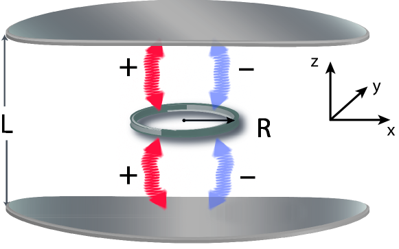
Figure 1: (Color online) Sketch of the system. A quantum ring of radius $R$ is placed inside a planar cavity of length $L$. The arrows with signs $+$ and $-$ correspond to clockwise and counterclockwise circularly polarized virtual photons.

The Hamiltonian of the considered electron-photon system has the form

$$\hat{\cal{H}}=\hat{\cal{H}}_{el}+\hat{\cal{H}}_{ph}+\hat{\cal{H}}_{int},$$ (1)

where $\hat{\cal{H}}_{el}$ is the Hamiltonian of an electron in the ring, $\hat{\cal{H}}_{ph}$ is the Hamiltonian of a photonic mode in the cavity, and $\hat{\cal{H}}_{int}$ is the Hamiltonian of electron-photon interaction.

The electron Hamiltonian is given by the expression

$$\hat{\cal{H}}_{el}=\frac{\hbar^{2}\hat{l}^{2}_{z}}{2m_{e}R^{2}},$$ (2)

where $m_{e}$ is the effective mass of electron in the ring, $R$ is the radius of the ring, $\hat{l}_{z}=-i\partial/\partial\varphi$ is operator of dimensionless electron angular momentum, and $\varphi$ is the angular coordinate of electron in the ring.

The photon Hamiltonian, accounting for both clockwise ($\lambda=+$) and counterclockwise ($\lambda=-$) circular polarizations, reads as

$$\hat{\cal{H}}_{ph} =\sum_{\mathbf{q},\eta,\lambda}\hbar\omega_{\mathbf{q},\eta,\lambda}\hat{a}^{\dagger}_{\mathbf{q},\eta,\lambda}\hat{a}_{\mathbf{q},\eta,\lambda}$$ (3)

$$+\sum_{\mathbf{q},\eta}\frac{\hbar\Omega_{LT}(\mathbf{q})}{2}(\hat{a}^{\dagger}_{\mathbf{q},\eta,+}\hat{a}_{\mathbf{q},\eta,-}+\hat{a}^{\dagger}_{\mathbf{q},\eta,-}\hat{a}_{\mathbf{q},\eta,+}),$$

where $\hat{a}^{\dagger}_{\mathbf{q},\eta,\lambda}$ and $\hat{a}_{\mathbf{q},\eta,\lambda}$ are creation and annihilation operators for cavity photons with polarizations $\lambda=\pm$ and wave vectors $(\mathbf{q},q_{z})$. Here $\mathbf{q}$ is the in-plane component of photon wave vector in the cavity, $q_{z}=\eta\pi/L$ is the quantized $z$ component of photon wave vector in the cavity, and $\eta=1,2,3,...$ is the number of photon mode in the cavity. Correspondingly, the first term in Eq. (3) describes the energy of cavity modes with dispersions given by

$$\omega_{\mathbf{q},\eta,\pm}=c_{\pm}\sqrt{q^{2}+q_{z}^{2}},$$ (4)

where $c_{\pm}=c/n_{\pm}$ are the speeds of light with clockwise and counterclockwise circular polarizations, and $n_{\pm}$ are the refractive indices for clockwise ($\lambda=+$) and counterclockwise ($\lambda=-$) polarized light. In what follows we will consider the case of chiral resonator. Thus, in general, $c_{+}\neq c_{-}$. As to the second term in Eq. (3), it describes the energy splitting between photon modes with different polarizations in a microcavity (longitudinal-transverse splitting).ShelykhRev The exact form of the longitudinal-transverse splitting function $\Omega_{LT}(\mathbf{q})$ depends on the construction of the resonator, but in majority of cases it can be approximated by the simple formula $\Omega_{LT}(\mathbf{q})=\hbar q^{2}/2\mu$, where $\mu=m_{TE}m_{TM}/(m_{TM}-m_{TE})$, $m_{TE}$ and $m_{TM}$ are the effective masses of cavity photons with TE and TM polarizations, respectively. For a typical microcavity structure, they can be found as $m_{TE}=3.68\times 10^{-4}m_{0}$ and $m_{TM}=3.62\times 10^{-4}m_{0}$, where $m_{0}$ is the mass of free electron.Kalita The presence of the longitudinal-transverse splitting affects the polarization of eigenmodes of the planar cavity, as it will be discussed below.

Taking into account one-dimensional geometry of the quantum ring, the interaction Hamiltonian has the form Kibis11

$$\hat{\cal{H}}_{int}=-eR\sum_{\mathbf{q},\eta,\lambda}\int\hat{\mathbf{E}}_{\mathbf{q},\eta,\lambda}\mathbf{t}(\varphi)d\varphi,$$ (5)

where the indefinite integral should be treated as an antiderivative of the subintegral function. Here $\mathbf{t}(\varphi)=-\mathbf{e}_{x}\sin\varphi+\mathbf{e}_{y}\cos\varphi$ is the unit tangent vector to the ring, $\mathbf{e}_{x}$ and $\mathbf{e}_{y}$ are the in-plane Cartesian unit vectors, the operator of the electric field in the cavity is

$$\hat{\mathbf{E}}_{\mathbf{q},\eta,\lambda}=i\sqrt{\frac{\hbar\omega_{\mathbf{q},\eta,\lambda}}{2\epsilon_{0}}}\left(\hat{a}_{\mathbf{q},\eta,\lambda}\mathbf{u}_{\mathbf{q},\eta,\lambda}-\hat{a}^{\dagger}_{\mathbf{q},\eta,\lambda}\mathbf{u}^{*}_{\mathbf{q},\eta,\lambda}\right),$$ (6)

eigenvectors of the cavity are given by the expression ScullyZubairy

$$\mathbf{u}_{\mathbf{q},\eta,\lambda}=\mathbf{e}_{\lambda,\mathbf{q}}\sqrt{\frac{2}{LS}}\sin\left(\frac{\pi\eta z}{L}\right)e^{i\mathbf{q}\cdot\mathbf{r}},$$ (7)

$L$ is the cavity length, $S$ is the cavity area, $\mathbf{r}$ is the in-plane radius vector, and $\mathbf{e}_{\lambda,\mathbf{q}}$ are the unit vectors of photon polarizations.

In order to describe the noninteracting electron-photon system in the cavity, let us use the jointed electron-photon space,KibisPRB $|m,N_{\mathbf{q},\eta,\lambda}\rangle=|m\rangle\otimes|N_{\mathbf{q},\eta,\lambda}\rangle$, which indicates that the electromagnetic field is in a quantum state with the photon occupation number $N_{\mathbf{q},\eta,\lambda}=0,1,2,3...$ , and the electron is in a quantum state with the wave function $\psi_{m}(\varphi)=1/\sqrt{2\pi}\exp(im\varphi)$, where $m=0,\pm 1,\pm 2...$ is the electron angular momentum along the ring axis. It should be noted that polarizations of eigenmodes of the photon Hamiltonian (3) are, in general, elliptical and strongly depend on in-plane photon wave vector $\mathbf{q}$, transforming into circular polarization for $q\rightarrow 0$ and into linear one for $q\rightarrow\infty$.ShelykhRev These elliptically polarized eigenmodes of the photon Hamiltonian (3) can be found using the Hopfield transformations:Haug

$$\hat{a}_{\mathbf{q},\eta,1}=\alpha_{\mathbf{q}}\hat{a}_{\mathbf{q},\eta,+}+\beta_{\mathbf{q}}\hat{a}_{\mathbf{q},\eta,-},$$ (8)

$$\hat{a}_{\mathbf{q},\eta,2}=\beta_{\mathbf{q}}\hat{a}_{\mathbf{q},\eta,+}-\alpha_{\mathbf{q}}\hat{a}_{\mathbf{q},\eta,-},$$ (9)

where the Hopfield coefficients can be written as

$$\alpha_{\mathbf{q}}=\frac{-\Omega_{LT}(\mathbf{q})}{\sqrt{\Omega_{LT}^{2}(\mathbf{q})+\left(\Delta_{\pm,\eta}(\mathbf{q})-\sqrt{\Delta_{\pm,\eta}^{2}(\mathbf{q})+\Omega_{LT}^{2}(\mathbf{q})}\,\right)^{2}}},$$ (10)

$$\beta_{\mathbf{q}}=\frac{\Delta_{\pm,\eta}(\mathbf{q})-\sqrt{\Delta_{\pm,\eta}^{2}(\mathbf{q})+\Omega_{LT}^{2}(\mathbf{q})}}{\sqrt{\Omega_{LT}^{2}(\mathbf{q})+\left(\Delta_{\pm,\eta}(\mathbf{q})-\sqrt{\Delta_{\pm,\eta}^{2}(\mathbf{q})+\Omega_{LT}^{2}(\mathbf{q})}\,\right)^{2}}},$$ (11)

and $\Delta_{\pm,\eta}(\mathbf{q})=\omega_{\mathbf{q},\eta,+}-\omega_{\mathbf{q},\eta,-}$. Correspondingly, eigenfrequencies of the cavity photon modes are

$$\omega_{\mathbf{q},\eta,1}=\frac{\omega_{\mathbf{q},\eta,+}+\omega_{\mathbf{q},\eta,-}}{2}+\frac{1}{2}\sqrt{\Delta_{\pm,\eta}^{2}(\mathbf{q})+\Omega_{LT}^{2}(\mathbf{q})},$$ (12)

$$\omega_{\mathbf{q},\eta,2}=\frac{\omega_{\mathbf{q},\eta,+}+\omega_{\mathbf{q},\eta,-}}{2}-\frac{1}{2}\sqrt{\Delta_{\pm,\eta}^{2}(\mathbf{q})+\Omega_{LT}^{2}(\mathbf{q})},$$ (13)

and the diagonalized photon Hamiltonian (3) reads as

$$\hat{\cal{H}}_{ph}=\sum_{\mathbf{q},\eta,\lambda^{\prime}}\hbar\omega_{\mathbf{q},\eta,\lambda^{\prime}}\hat{a}^{\dagger}_{\mathbf{q},\eta,\lambda^{\prime}}\hat{a}_{\mathbf{q},\eta,\lambda^{\prime}},$$ (14)

where $\lambda^{\prime}=1,2$ is the polarization index of the above-mentioned elliptical basis. As a result, the energy spectrum of the noninteracting electron-photon system in the cavity is

$$\varepsilon_{m,N_{\mathbf{q},\eta,\lambda^{\prime}}}^{(0)}=\frac{\hbar^{2}m^{2}}{2m_{e}R}+N_{\mathbf{q},\eta,\lambda^{\prime}}\hbar\omega_{\mathbf{q},\eta,\lambda^{\prime}}.$$ (15)

For the case of electromagnetic vacuum in the cavity, photon occupation numbers in Eq. (15) are $N_{\mathbf{q},\eta,\lambda^{\prime}}=0$. Considering the electron interaction with the photon vacuum as a weak perturbation described by the Hamiltonian (5), we can apply the conventional perturbation theory. Then the energy spectrum of electron in the ring dressed by vacuum fluctuations is given by

$$\varepsilon_{m,0}= \varepsilon_{m,0}^{(0)}+\sum_{\mathbf{q},m^{\prime},\eta}\left(\frac{|\langle m^{\prime},1_{\mathbf{q},\eta,1}|\hat{\cal{H}}_{int}|m,0\rangle|^{2}}{\varepsilon_{m,0}^{(0)}-\varepsilon_{m^{\prime},1_{\mathbf{q},\eta,1}}}\right.$$

$$+\left.\frac{|\langle m^{\prime},1_{\mathbf{q},\eta,2}|\hat{\cal{H}}_{int}|m,0\rangle|^{2}}{\varepsilon_{m,0}^{(0)}-\varepsilon_{m^{\prime},1_{\mathbf{q},\eta,2}}}\right).$$ (16)

Writing the interaction Hamiltonian (5) for the elliptical polarizations $\lambda=1,2$ and assuming the ring to be placed in the center of the cavity, the expression for the electron energy spectrum (16) takes the final form (see detailed derivation in Appendix A):

$$\varepsilon_{m,0}=\varepsilon_{m,0}^{(0)}+\sum_{m^{\prime},\eta}\frac{e^{2}R^{2}}{2\pi}\frac{1}{2\epsilon_{0}L}\frac{1}{(m-m^{\prime})^{2}}$$ (17)

$$\times\Bigg{(}\int\limits_{0}^{\infty}dq\frac{q\hbar\omega_{q,\eta,1}(J_{m-m^{\prime}-1}^{2}(qR)\alpha_{q}^{2}+J_{m-m^{\prime}+1}^{2}(qR)\beta_{q}^{2})}{[\varepsilon_{R}(m^{2}-m^{\prime 2})-\hbar\omega_{q,\eta,1}]}$$

$$+\int\limits_{0}^{\infty}dq\frac{q\hbar\omega_{q,\eta,1}(J_{m-m^{\prime}-1}^{2}(qR)\beta_{q}^{2}+J_{m-m^{\prime}+1}^{2}(qR)\alpha_{q}^{2})}{[\varepsilon_{R}(m^{2}-m^{\prime 2})-\hbar\omega_{q,\eta,2}]}\Bigg{)},$$

where $\varepsilon_{R}=\hbar^{2}/2m_{e}R^{2}$ is the characteristic electron energy in the ring, and $\eta=1,3,5,...$ is odd integer.

III Discussion

It should be noted that the integrals in Eq. (17) are divergent. This divergency arises from the accounting of infinite number of vacuum modes and has the same origin as a formally infinite energy of vacuum state in the cavity. However, the physically measurable quantity is not the shift of electron energy levels but the splitting of them by vacuum fluctuations. Particularly, the splitting of electron energy levels with mutually opposite angular momenta $m$ and $-m$,

$$\Delta\varepsilon=|\varepsilon_{m,0}-\varepsilon_{-m,0}|,$$ (18)

is finite quantity which can be calculated with Eq. (17) numerically.

It follows from the time-reversal symmetry that clockwise and counterclockwise polarized photons shift electron energy levels of the ring with angular momenta $m$ and $-m$ equally. Indeed, the eigenfrequencies (4) for clockwise and counterclockwise circularly polarized photons are equal in the vacuum, $\omega_{\mathbf{q},\eta,+}=\omega_{\mathbf{q},\eta,-}$. According to Eq. (17), in this case we have the equality $\varepsilon_{m,0}=\varepsilon_{-m,0}$ and the splitting (18) vanishes. Therefore, the energy splitting needs the breaking of the symmetry between virtual photons with different circular polarizations. This can be achieved with filling the cavity with an optically active medium, where the refractive indices $n_{+}$ and $n_{-}$ are different. In what follows we will consider a metallic quantum ring placed inside the cavity filled with such an optically active medium. Let electron states with angular momenta $m$ and $-m$ lie at the Fermi level $\mu$ of the ring when the electron-photon interaction is absent (see Fig. 2a). Then, summarizing in Eq. (17) over states $m^{\prime}$ lying over the Fermi level, we can obtain the vacuum-induced splitting between otherwise degenerate states $m$ and $-m$ (see Fig. 2b). As a result of the lifting of the degeneracy, the ground state of the electron system in the ring possesses well-defined angular momentum which corresponds to the nonzero electric current

$$j=\frac{me\hbar}{2\pi R^{2}m_{e}}.$$ (19)

Since the current (19) is associated with the ground state, it flows without any dissipation and is persistent. The experimental observability of the vacuum-induced persistent current depends on optimal choice of an optically active medium filling the cavity, since the splitting (18) depends on the difference of the refractive indices, $\Delta n=|n_{+}-n_{-}|$ (see Fig. 2c). For instance, the cavity can be filled with a magnetogyrotropic medium based on ferrite garnets, where $\Delta n\approx 5\times 10^{-3}$ (see Ref. [Ferrite, ]). In this case, the vacuum-induced splitting (18) can be estimated as $\Delta\varepsilon\sim 1~{}\mu$eV that is comparable to the value of vacuum-induced Lamb shift in atoms.Lamb_47 ; Bethe_47 ; Scully_10 The effect becomes even more pronounced if the cavity is filled with an active media with the circular dichroism CD_monography or media based on a metamaterial with a giant optical activity.Zheludev1 Then, one of the two circularly polarized photon modes in the cavity is suppressed and its contribution to the energy splitting (18) can be neglected, which leads to the drastic increase of the splitting. In this case, for $|m|\sim 10^{3}$ the splitting is $\Delta\varepsilon\sim 1$ meV (see Figs. 2d and 2e). Therefore, the condition of observability of the vacuum-induced persistent current, $\Delta\varepsilon\gg T$, can be easily satisfied at liquid helium temperatures $T$.

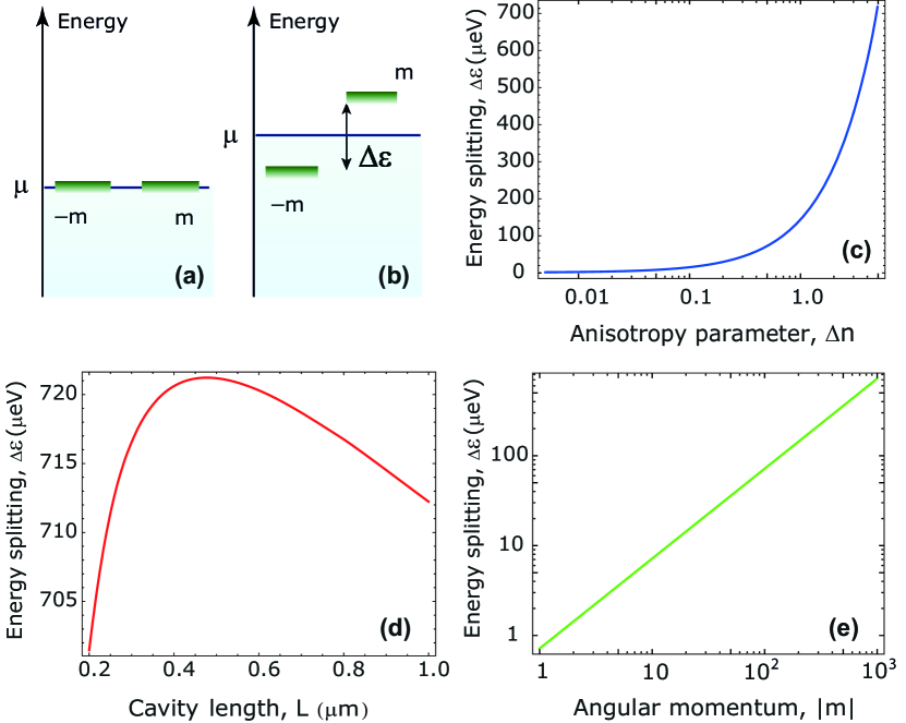
Figure 2: (Color online) (a) Structure of energy levels close to the Fermi level $\mu$ in the ring placed outside the cavity; (b) Structure of energy levels close to the Fermi level $\mu$ in the ring placed inside the cavity filled with an optically active medium; (c) Vacuum-induced energy splitting for electron states with $|m|=10^{3}$ as a function of the anisotropy parameter of the optically active medium, $\Delta n=|n_{+}-n_{-}|$, in the cavity with $L=0.4~{}\mu$m; (d) Vacuum-induced energy splitting for electron states with $|m|=10^{3}$ as a function of cavity length $L$ for the case of fully suppressed counterclockwise circularly polarized mode; (e) Vacuum-induced energy splitting as a function of angular momentum $|m|$ at the Fermi level of the ring for the case of fully suppressed counterclockwise circularly polarized mode in the cavity with $L=0.4~{}\mu$m.

To clarify the physical nature of the discussed effect, it should be noted that the persistent current (19) arises from the broken time-reversal symmetry in a chiral microcavity. Indeed, the broken time-reversal symmetry leads to physical nonequivalence of electron motion for mutually opposite directions in various nanostructures: quantum wells, Gorbatsevich_93 ; Aleshchenko_93 ; Omelyanovskii_96 ; Kibis_97 ; Kibis_98_1 ; Kibis_98_2 ; Kibis_99 ; Kibis_00 ; Diehl_07 ; Diehl_09 ; Kibis12 quantum wires, Kibis11 carbon nanotubes, Kibis_93 ; Kibis_01_1 ; Kibis_01_2 quantum rings, Buttiker ; Mailly ; Kibis11 hybrid semiconductor-ferromagnet nanostructures, Lawton_02 etc. As a result, a ground-state current (persistent current) can exist in such nanostructures. Buttiker ; Mailly ; Kibis11 ; Kibis12 Particularly, clockwise and counterclockwise electron rotations in the quantum ring placed inside the chiral microcavity are nonequivalent and, therefore, the persistent current (19) appears.

For the ring with the radius $R\approx 50$ nm and electron angular momentum at the Fermi level $|m|\approx 1000$, the vacuum-induced persistent current (19) can be estimated as $j\approx 1$ $\mu$A. The magnetic field induced by the current can be detected experimentally with a standard superconducting quantum interference device (SQUID). In order to detect the current and to exclude influence of the SQUID on the phenomenon, the SQUID should be near a microcavity but outside it. Since the time-reversal symmetry is broken in an optically active material filling the microcavity, a built-in magnetic field can exist there. In order to separate the magnetic field generated by the vacuum-induced persistent current from other possible contributions, difference-scheme measurements can be used. For instance, magnetic-field measurements can be done for the microcavity with two mirrors (where the vacuum-induced persistent current exists) and for the same cavity with a removed mirror (where the vacuum-induced persistent current is absent). Using of compensation-scheme measurements — where the built-in magnetic field is compensated by an opposite directed magnetic field — is also possible.

The magnetic moment of a ring with the persistent current (19) is given by

$$M=\frac{me\hbar}{2m_{e}}.$$ (20)

Due to the vacuum-induced magnetic moment (20), the ring in the cavity behaves as an artificial “spin”. Replacing a single ring with more complicated structure consisting of an array of rings, which can be constructed experimentally,Zheludev2 we will have an artificially designed Ising magnet. Thus, the proposed structure forms a basis for the novel concept of optical metamagnets which are expected to have intriguing properties. In particular, it was recently demonstrated that resonator-based systems with broken time-reversal symmetry can allow observation of non-trivial topological phases of light.Yiddong The detail investigation of these effects, however, goes beyond the scopes of the present paper and will be done elsewhere.

IV Conclusion

Summarizing the aforesaid, we considered the novel quantum electrodynamical effect emerging due to the interaction of electrons in a quantum ring and electromagnetic vacuum fluctuations in a resonator. We have shown that in the case of the broken symmetry between clockwise and counterclockwise circular polarizations of photon modes in the cavity, dressed electronic states in the ring with opposite angular momenta are split in energy. This vacuum-induced splitting leads to the circulation of persistent current in the ring. Subsequently, magnetic field generated by the persistent current can be detected by SQUID techniques, that allows to claim the discussed phenomenon as a first macroscopically observable vacuum effect in nanostructures. As to possible applications of the effect to devices, an array of quantum rings can be considered as a novel type of metamaterial with magnetic properties (optical metamagnet). It should be noted that the discussed effect is of general character and will take place in any nanostructures which are topologically homeomorphous to ring (particularly, in carbon nanotubes).

Appendix A Derivation of basic expressions

In order to derive Eq. (17) from Eq. (16), we need to find the matrix elements $\langle m^{\prime},1_{\mathbf{q},\eta,1}|\hat{\cal{H}}_{int}|m,0\rangle$ and $\langle m^{\prime},1_{\mathbf{q},\eta,2}|\hat{\cal{H}}_{int}|m,0\rangle$. To reach this aim, we have to write the interaction Hamiltonian (5) in the elliptical polarization basis $\lambda=1,2$. Using relations (8)–(9) written in the form $\mathbf{e}_{1,\mathbf{q}}=\alpha_{\mathbf{q}}\mathbf{e}_{+}+\beta_{\mathbf{q}}\mathbf{e}_{-}$ and $\mathbf{e}_{2,\mathbf{q}}=\beta_{\mathbf{q}}\mathbf{e}_{+}-\alpha_{\mathbf{q}}\mathbf{e}_{-}$, the electric field operators of the cavity mode, $\hat{\mathbf{E}}_{\mathbf{q},\eta,\lambda}$, can be written in the Hamiltonian (5) as

$$\hat{\mathbf{E}}_{\mathbf{q},\eta,1} = i\sqrt{\frac{\hbar\omega_{\mathbf{q},\eta,1}}{\epsilon_{0}LS}}\Big{(}\hat{a}_{\mathbf{q},\eta,1}\alpha_{\mathbf{q}}e^{i\mathbf{q}\cdot\mathbf{r}}\mathbf{e}_{+}+\hat{a}_{\mathbf{q},\eta,1}\beta_{\mathbf{q}}e^{i\mathbf{q}\cdot\mathbf{r}}\mathbf{e}_{-}-\hat{a}^{\dagger}_{\mathbf{q},\eta,1}\alpha_{\mathbf{q}}e^{-i\mathbf{q}\cdot\mathbf{r}}\mathbf{e}_{-}-\hat{a}^{\dagger}_{\mathbf{q},\eta,1}\beta_{\mathbf{q}}e^{-i\mathbf{q}\cdot\mathbf{r}}\mathbf{e}_{+}\Big{)}\sin\left(\frac{\pi\eta z}{L}\right),$$ (21)

$$\hat{\mathbf{E}}_{\mathbf{q},\eta,2} = i\sqrt{\frac{\hbar\omega_{\mathbf{q},\eta,2}}{\epsilon_{0}LS}}\Big{(}\hat{a}_{\mathbf{q},\eta,2}\beta_{\mathbf{q}}e^{i\mathbf{q}\cdot\mathbf{r}}\mathbf{e}_{+}-\hat{a}_{\mathbf{q},\eta,2}\alpha_{\mathbf{q}}e^{i\mathbf{q}\cdot\mathbf{r}}\mathbf{e}_{-}-\hat{a}^{\dagger}_{\mathbf{q},\eta,2}\beta_{\mathbf{q}}e^{-i\mathbf{q}\cdot\mathbf{r}}\mathbf{e}_{-}+\hat{a}^{\dagger}_{\mathbf{q},\eta,2}\alpha_{\mathbf{q}}e^{-i\mathbf{q}\cdot\mathbf{r}}\mathbf{e}_{+}\Big{)}\sin\left(\frac{\pi\eta z}{L}\right),$$ (22)

where $\mathbf{e}_{\pm}=(\mathbf{e}_{x}\pm i\mathbf{e}_{y})/\sqrt{2}$ are the unit vectors corresponding to clockwise and counterclockwise circular polarizations of cavity photons. Taking into account Eqs. (21)–(22) and keeping in mind that $\mathbf{e}_{+}\cdot\mathbf{t}(\varphi)=ie^{i\varphi}/\sqrt{2}$ and $\mathbf{e}_{-}\cdot\mathbf{t}(\varphi)=-ie^{-i\varphi}/\sqrt{2}$, the interaction Hamiltonian (5) reads as

$$\hat{\cal{H}}_{int} = -ieR\sum_{\mathbf{q},\eta}\left[\sqrt{\frac{\hbar\omega_{\mathbf{q},\eta,1}}{2\epsilon_{0}LS}}\left(i\int\hat{a}_{\mathbf{q},\eta,1}\alpha_{\mathbf{q}}e^{i\mathbf{q}\cdot\mathbf{r}}e^{i\varphi}d\varphi-i\int\hat{a}_{\mathbf{q},\eta,1}\beta_{\mathbf{q}}e^{i\mathbf{q}\cdot\mathbf{r}}e^{-i\varphi}d\varphi+i\int\hat{a}^{\dagger}_{\mathbf{q},\eta,1}\alpha_{\mathbf{q}}e^{-i\mathbf{q}\cdot\mathbf{r}}e^{-i\varphi}d\varphi\right.\right.$$ (23)

$$- \left.i\int\hat{a}^{\dagger}_{\mathbf{q},\eta,1}\beta_{\mathbf{q}}e^{-i\mathbf{q}\cdot\mathbf{r}}e^{i\varphi}d\varphi\right)+\sqrt{\frac{\hbar\omega_{\mathbf{q},\eta,2}}{2\epsilon_{0}LS}}\left(i\int\hat{a}_{\mathbf{q},\eta,2}\beta_{\mathbf{q}}e^{i\mathbf{q}\cdot\mathbf{r}}e^{i\varphi}d\varphi+i\int\hat{a}_{\mathbf{q},\eta,2}\alpha_{\mathbf{q}}e^{i\mathbf{q}\cdot\mathbf{r}}e^{-i\varphi}d\varphi\right.$$

$$+ \left.\left.i\int\hat{a}^{\dagger}_{\mathbf{q},\eta,2}\beta_{\mathbf{q}}e^{-i\mathbf{q}\cdot\mathbf{r}}e^{-i\varphi}d\varphi+i\int\hat{a}_{\mathbf{q},\eta,2}\alpha_{\mathbf{q}}e^{-i\mathbf{q}\cdot\mathbf{r}}e^{i\varphi}d\varphi\right)\right]\sin\left(\frac{\pi\eta z}{L}\right).$$

In what follows we will assume that the quantum ring is placed in the center of the cavity ($z=L/2$). Consequently, the sine in the last line of Eq. (23) can be omitted and the summation over the index $\eta$ in Eq. (23) should be performed over odd integer numbers. To proceed the derivation, we have to rewrite the exponents $e^{\pm i\mathbf{q}\cdot\mathbf{r}}$ in Eq. (23) using the polar coordinates $\mathbf{r}=(R,\varphi)$ and $\mathbf{q}=(q,\theta)$. Then the exponents can be written as $e^{\pm i\mathbf{q}\cdot\mathbf{r}}=e^{\pm iqR\cos(\theta-\varphi)}$. Let us use the Jacobi-Anger expansion Gradstein

$$e^{ix\cos\xi}=\sum_{n=-\infty}^{\infty}(i)^{n}J_{n}(x)e^{in\xi},$$

where $J_{n}(x)$ is the Bessel function of the first kind. Then we arrive to the expression

$$e^{iqR\cos(\varphi-\theta)}=\sum_{n=-\infty}^{\infty}(i)^{n}J_{n}(qR)e^{in(\varphi-\theta)}.$$

Using the well-known property of the Bessel function, $J_{-n}(x)=(-1)^{n}J_{n}(x)$, the complex conjugation of this exponent can be written as

$$e^{-iqR\cos(\varphi-\theta)}=\sum_{n=-\infty}^{\infty}(i)^{-n}J_{n}(qR)e^{in(\varphi-\theta)}.$$

As a result, the Hamiltonian (23) takes the form

$$\hat{\cal{H}}_{int} = eR\sum_{\mathbf{q},\eta}\sum_{n=-\infty}^{\infty}J_{n}(qR)e^{in\theta}\left[\sqrt{\frac{\hbar\omega_{\mathbf{q},\eta,1}}{2\epsilon_{0}LS}}\left(\hat{a}_{\mathbf{q},\eta,1}\alpha_{\mathbf{q}}(i)^{n}\int e^{-i(n-1)\varphi}d\varphi-\hat{a}_{\mathbf{q},\eta,1}\beta_{\mathbf{q}}(i)^{n}\int e^{-i(n+1)\varphi}d\varphi\right.\right.$$ (24)

$$+ \hat{a}^{\dagger}_{\mathbf{q},\eta,1}\alpha_{\mathbf{q}}(i)^{-n}\int e^{-i(n+1)\varphi}d\varphi-\hat{a}^{\dagger}_{\mathbf{q},\eta,1}\beta_{\mathbf{q}}(i)^{-n}\left.\int e^{-i(n-1)\varphi}d\varphi\right)+\sqrt{\frac{\hbar\omega_{\mathbf{q},\eta,2}}{2\epsilon_{0}LS}}\left(\hat{a}_{\mathbf{q},\eta,2}\beta_{\mathbf{q}}(i)^{n}\int e^{-i(n-1)\varphi}d\varphi\right.$$

$$+ \left.\hat{a}_{\mathbf{q},\eta,2}\alpha_{\mathbf{q}}(i)^{n}\int e^{-i(n+1)\varphi}d\varphi+\hat{a}^{\dagger}_{\mathbf{q},\eta,2}\beta_{\mathbf{q}}(i)^{-n}\int e^{-i(n+1)\varphi}d\varphi+\hat{a}^{\dagger}_{\mathbf{q},\eta,2}\alpha_{\mathbf{q}}(i)^{-n}\int e^{-i(n-1)\varphi}\left.d\varphi\right)\right].$$

Performing in Eq. (24) trivial integration over electron angular coordinate $\varphi$, we arrive to the expression

$$\hat{\cal{H}}_{int} = eR\sum_{\mathbf{q},\eta}\sum_{n=-\infty}^{\infty}J_{n}(qR)e^{in\theta}\left[\sqrt{\frac{\hbar\omega_{\mathbf{q},\eta,1}}{2\epsilon_{0}LS}}\left(\hat{a}_{\mathbf{q},\eta,1}\alpha_{\mathbf{q}}(i)^{n+1}\frac{e^{-i(n-1)\varphi}}{n-1}-\hat{a}_{\mathbf{q},\eta,1}\beta_{\mathbf{q}}(i)^{n+1}\frac{e^{-i(n+1)\varphi}}{n+1}\right.\right.$$ (25)

$$+ \left.\hat{a}^{\dagger}_{\mathbf{q},\eta,1}\alpha_{\mathbf{q}}(i)^{-(n-1)}\frac{e^{-i(n+1)\varphi}}{n+1}-\hat{a}^{\dagger}_{\mathbf{q},\eta,1}\beta_{\mathbf{q}}(i)^{-(n-1)}\frac{e^{-i(n-1)\varphi}}{n-1}\right)+\sqrt{\frac{\hbar\omega_{\mathbf{q},\eta,2}}{2\epsilon_{0}LS}}\left(\hat{a}_{\mathbf{q},\eta,2}\beta_{\mathbf{q}}(i)^{n+1}\frac{e^{-i(n-1)\varphi}}{n-1}\right.$$

$$+ \left.\hat{a}_{\mathbf{q},\eta,2}\alpha_{\mathbf{q}}(i)^{n+1}\frac{e^{-i(n+1)\varphi}}{n+1}+\left.\hat{a}^{\dagger}_{\mathbf{q},\eta,2}\beta_{\mathbf{q}}(i)^{-(n-1)}\frac{e^{-i(n+1)\varphi}}{n+1}+\hat{a}^{\dagger}_{\mathbf{q},\eta,2}\alpha_{\mathbf{q}}(i)^{-(n-1)}\frac{e^{-i(n-1)\varphi}}{n-1}\right)\right].$$

The matrix element of the Hamiltonian (25) for virtual photons with the polarization $\lambda=1$ is

$$\langle m^{\prime},1_{\mathbf{q},\eta,1}|\hat{\cal{H}}_{int}|m,0\rangle = eR\sqrt{\frac{\hbar\omega_{\mathbf{q},\eta,1}}{2\varepsilon_{0}LS}}\sum_{n=-\infty}^{\infty}(i)^{-(n-1)}J_{n}(qR)e^{in\theta}\left[\frac{\alpha_{\mathbf{q}}}{n+1}\int\limits_{0}^{2\pi}\frac{d\varphi}{2\pi}e^{i(m-m^{\prime}-n-1)\varphi}\right.$$ (26)

$$- \left.\frac{\beta_{\mathbf{q}}}{n-1}\int\limits_{0}^{2\pi}\frac{d\varphi}{2\pi}e^{i(m-m^{\prime}-n+1)\varphi}\right].$$

The integration over the angular coordinate $\varphi$ in Eq. (26) gives the Kronecker deltas $\delta_{n,m-m^{\prime}-1}$ and $\delta_{n,m-m^{\prime}+1}$, which reduce the summation over the index $n$ in Eq. (26) to the single term:

$$\langle m^{\prime},1_{\mathbf{q},\eta,1}|\hat{\cal{H}}_{int}|m,0\rangle=-eR\sqrt{\frac{\hbar\omega_{\mathbf{q},\eta,1}}{2\varepsilon_{0}LS}}\frac{(i)^{-(m-m^{\prime})}}{m-m^{\prime}}e^{i(m-m^{\prime})\theta}\left[\alpha_{\mathbf{q}}J_{m-m^{\prime}-1}(qR)e^{-i\theta}+\beta_{\mathbf{q}}J_{m-m^{\prime}+1}(qR)e^{i\theta}\right].$$ (27)

Deriving the matrix element of the interaction Hamiltonian (25) for virtual photons with the polarization $\lambda=2$ in the same way, we arrive to the expression

$$\langle m^{\prime},1_{\mathbf{q},\eta,2}|\hat{\cal{H}}_{int}|m,0\rangle=-eR\sqrt{\frac{\hbar\omega_{\mathbf{q},\eta,2}}{2\varepsilon_{0}LS}}\frac{(i)^{-(m-m^{\prime})}}{m-m^{\prime}}e^{i(m-m^{\prime})\theta}\left[\beta_{\mathbf{q}}J_{m-m^{\prime}-1}(qR)e^{-i\theta}-\alpha_{\mathbf{q}}J_{m-m^{\prime}+1}(qR)e^{i\theta}\right].$$ (28)

Substituting Eqs. (27)–(28) into Eq. (16) and passing from summation over photon wave vectors $\mathbf{q}$ to integration, $\sum_{\mathbf{q}}\rightarrow S/(2\pi)^{2}\int_{0}^{\infty}qdq\int_{0}^{2\pi}d\theta$, we arrive to Eqs. (17)–(18) which are the basic expressions for the analysis of the discussed effect.

References

- (1) P. W. Milonni, The Quantum Vacuum (Academic, New York, 1994).
- (2) W. E. Lamb and R. C. Retherford, Phys. Rev. 72, 241 (1947).
- (3) H. A. Bethe, Phys. Rev. 72, 339 (1947).
- (4) M. O. Scully and A. A. Svidzinsky, Science 328, 1239 (2010).
- (5) H. B. G. Casimir, Kon. Ned. Akad. Wetensch. Proc. 51, 793 (1948).
- (6) I. V. Fialkovsky, V. N. Marachevsky, and D. V. Vassilevich, Phys. Rev. B 84, 035446 (2011).
- (7) B. E. Sernelius, EPL 95, 57003 (2011).
- (8) R. L. Jaffe, Phys. Rev. D 72, 021301 (2005).
- (9) S. M. Dutra, Cavity Quantum Electrodynamics (Wiley, Hoboken, 2005).
- (10) H. Walther, B. T. H. Varcoe, B.-G. Englert, and T. Becker, Rep. Prog. Phys. 69 1325 (2006).
- (11) W. E. Lamb, W. P. Schleich, M. O. Scully, C. H. Townes, Rev. Mod. Phys. 71, S263 (1999).
- (12) R. E. Slusher, Rev. Mod. Phys. 71, S471 (1999).
- (13) A. V. Kavokin, J. J. Baumberg, G. Malpuech, and F. P. Laussy, Microcavities (Oxford University Press, Oxford, 2007).
- (14) T. C. H. Liew, I. A. Shelykh, and G. Malpuech, Physica E 43, 1543 (2011).
- (15) C. Cohen-Tannoudji, J. Dupont-Roc, G. Grynberg, Atom-Photon Interactions: Basic Processes and Applications (Wiley, Chichester, 1998).
- (16) S. H. Autler and C. H. Townes, Phys. Rev. 100, 703 (1955).
- (17) M. O. Scully and M. S. Zubairy, Quantum Optics (Cambridge University Press, Cambridge, 2001).
- (18) M. Lindberg and S. W. Koch, Phys. Rev. B 38, 7607 (1988).
- (19) J. F. Dynes, M. D. Frogley, M. Beck, J. Faist, and C. C. Phillips, Phys. Rev. Lett. 94, 157403 (2005).
- (20) Y. Wu and X. Yang, Phys. Rev. Lett. 98, 013601 (2007).
- (21) O. V. Kibis, Phys. Rev. B 81, 165433 (2010).
- (22) O. V. Kibis, Phys. Rev. Lett. 107, 106802 (2011).
- (23) O. V. Kibis, Phys. Rev. B 86, 155108 (2012).
- (24) O. Jonasson, C.-S. Tang, H.-S. Goan, A. Manolescu, and V. Gudmundsson, New J. Phys. 14 013036, (2012).
- (25) A. Hayat, C. Lange, L. A. Rozema, A. Darabi, H. M. van Driel, A. M. Steinberg, B. Nelsen, D. W. Snoke, L. N. Pfeiffer, and K. W. West, Phys. Rev. Lett. 109, 033605 (2012).
- (26) M. Buttiker, Y. Imry, R. Landauer, Phys. Lett. A 96, 365 (1983).
- (27) D. Mailly, C. Chapelier, and A. Benoit, Phys. Rev. Lett. 70, 2020 (1993).
- (28) O. V. Kibis, O. Kyriienko, and I. A. Shelykh, Phys. Rev. B 84, 195413 (2011).
- (29) I. A. Shelykh, A. V. Kavokin, Y. G. Rubo, T. C. H. Liew, and G. Malpuech, Sem. Sci. Technol. 25, 013001 (2010).
- (30) H. Deng, H. Haug, and Y. Yamamoto, Rev. Mod. Phys. 82, 1489 (2010).
- (31) M. Kaliteevski, S. Brand, R. A. Abram, I. Iorsh, A. V. Kavokin, and I. A. Shelykh, Appl. Phys. Lett. 95, 251108 (2009).
- (32) P. S. Pershan, J. Appl. Phys. 38, 1482 (1967).
- (33) P. J. Stephens, Ann. Rev. Phys. Chem. 25, 201 (1974).
- (34) E. Plum, J. Zhou, J. Dong, V. A. Fedotov, T. Koschny, C. M. Soukoulis, and N. I. Zheludev, Phys. Rev. B 79, 035407 (2009).
- (35) A. A. Gorbatsevich, V. V. Kapaev, Y. V. Kapaev, JETP Lett. 57, 580 (1993).
- (36) Yu. A. Aleshchenko, I. D. Voronova, S. P. Grishechkina, V. V. Kapaev, Yu. V. Kopaev, I. V. Kucherenko, V. I. Kadushkin, S. I. Fomichev, JETP Lett. 58, 384 (1993).
- (37) O. E. Omelyanovskii, V. I. Tsebro, V. I. Kadushkin, JETP Lett. 63, 209 (1996).
- (38) O. V. Kibis, JETP Lett. 66, 588 (1997).
- (39) O. V. Kibis, Phys. Lett. A 237, 292 (1998).
- (40) O. V. Kibis, Phys. Lett. A 244, 432 (1998).
- (41) O. V. Kibis, JETP 88, 527 (1999).
- (42) A. G. Pogosov, M. V. Budantsev, O. V. Kibis, A. Pouydebasque, D. K. Maude, J. C. Portal, Phys. Rev. B 61, 15603 (2000).
- (43) H. Diehl, V. A. Shalygin, S. N. Danilov, S. A. Tarasenko, V. V. Bel’kov, D. Schuh, W. Wegscheider, W. Prettl, S. D. Ganichev, J. Phys.: Condens. Matter 19, 436232 (2007).
- (44) H. Diehl, V. A. Shalygin, L.E. Golub, S. A. Tarasenko, S. N. Danilov, V. V. Bel’kov, E. G. Novik, H. Buhmann, C. Brüne, L. W. Molenkamp, E. L. Ivchenko, and S. D. Ganichev, Phys. Rev. B 80, 075311 (2009).
- (45) D. A. Romanov, O. V. Kibis, Phys. Lett. A 178, 335 (1993).
- (46) O. V. Kibis, Physica E 12, 741 (2001).
- (47) O. V. Kibis, Phys. Sol. State 43, 2336 (2001).
- (48) D. Lawton, A. Nogaret, M. V. Makarenko, O. V. Kibis, S. J. Bending, M. Henini, Physica E 13, 669 (2002).
- (49) E. Plum, X.-X. Liu, V. A. Fedotov, Y. Chen, D. P. Tsai, and N. I. Zheludev, Phys. Rev. Lett. 102, 113902 (2009).
- (50) G. Q. Liang, Y. D. Chong, arXiv:1212.5034 (2013).
- (51) I. S. Gradstein and I. H. Ryzhik, Table of Series, Products and Integrals (Academic Press, New York, 2007).