ERROR EMITTANCE AND ERROR TWISS FUNCTIONS IN THE PROBLEM OF RECONSTRUCTION OF DIFFERENCE ORBIT PARAMETERS BY USAGE OF BPM’S WITH FINITE RESOLUTION

Abstract

The problem of errors, arising due to finite BPM resolution, in the difference orbit parameters, which are found as a least squares fit to the BPM data, is one of the standard problems of the accelerator physics. In this article we present a “dynamical point of view” on this problem, which allows us to describe properties of the BPM measurement system in terms of the usual accelerator physics concepts of emittance and betatron functions.

1 INTRODUCTION

The determination of variations in the transverse beam position and in the beam energy using readings of beam position monitors (BPMs) is one of the standard and important problems of accelerator physics. If the optical model of the beam line and BPM resolutions are known, the typical choice is to let jitter parameters be a solution of the weighted linear least squares problem. Even so for the case of transversely uncoupled motion this least squares problem can be solved “by hand” (see, for example  [2, 3]), the direct usage of obtained analytical solution as a tool for designing of a “good measurement system” does not look to be fairly straightforward. It seems that a better understanding of the nature of the problem is still desirable.

A step in this direction was made in the papers  [4, 5], where dynamic was introduced into this problem which in the beginning seemed to be static. When one changes the position of the reconstruction point, the estimate of the jitter parameters propagates along the beam line exactly as a particle trajectory and it becomes possible (for every fixed jitter values) to consider a virtual beam consisting from virtual particles obtained as a result of application of least squares reconstruction procedure to “all possible values” of BPM reading errors. The dynamics of the centroid of this beam coincides with the dynamics of the true difference orbit and the covariance matrix of the jitter reconstruction errors can be treated as the matrix of the second central moments of this virtual beam distribution.

In accelerator physics a beam is characterized by its emittances, energy spread, dispersions, betatron functions and etc. All these values immediately become the properties of the BPM measurement system. In this way one can compare two BPM systems comparing their error emittances and error energy spreads, or, for a given measurement system, one can achieve needed balance between coordinate and momentum reconstruction errors by matching the error betatron functions in the point of interest to the desired values. In this article we illustrate this dynamical point of view on the BPM measurement system considering the case of transversely uncoupled nondispersive beam motion (inclusion of the energy degree of freedom and multiple examples can be found in cited above papers  [4, 5]). As application, we formulate requirements on the BPM measurement system of the high-energy intra-bunch-train feedback system (IBFB) of the European X-Ray Free-Electron Laser (XFEL) Facility in terms of introduced concepts of error emittance and error Twiss parameters  [6, 7].

2 STANDARD LEAST SQUARES SOLUTION

We will assume that the transverse particle motion is uncoupled in linear approximation and will use the variables $\,\vec{z}=(x,\,p_{x})^{\top}\,$ for the description of the horizontal beam oscillations. As orbit parameters we will understand values of $\,x\,$ and $\,p_{x}\,$ given in some predefined point in the beam line (reconstruction point with longitudinal position $\,s=r\,$) and as transverse jitter in this point we will mean the difference $\,\delta\vec{z}(r)=\left(x(r)-\bar{x}(r),\,p_{x}(r)-\bar{p}_{x}(r)\right)^{\top}$ between parameters of the instantaneous orbit and parameters of some predetermined “golden trajectory” $(\bar{x},\,\bar{p}_{x})^{\top}$.

Let us assume that we have $n$ BPMs in our beam line placed at positions $\,s_{1},\ldots,s_{n}\,$ and they deliver readings $\vec{b}_{c}=\left(b_{1}^{c},\ldots,b_{n}^{c}\right)^{\top}$ for the current trajectory with previously recorded observations for the golden orbit being $\vec{b}_{g}=\left(b_{1}^{g},\ldots,b_{n}^{g}\right)^{\top}$. Suppose that the difference between these readings can be represented in the form

$$\delta\vec{b}_{\varsigma}\,\stackrel{{\scriptstyle\rm def}}{{=}}\,\vec{b}_{c}\,-\,\vec{b}_{g}\,=\,\left(\begin{array}[]{c}x(s_{1})-\bar{x}(s_{1})\\ \vdots\\ x(s_{n})-\bar{x}(s_{n})\end{array}\right)\,+\,\vec{\,\varsigma},$$ (4)

where the random vector $\vec{\,\varsigma}=(\varsigma_{1},\ldots,\varsigma_{n})^{\top}$ has zero mean and positive definite covariance matrix $V_{\varsigma}$.

Let $\,A_{m}(r)\,$ be a symplectic transfer matrix from location of the reconstruction point to the $m$-th BPM location

$$A_{m}(r)\,=\,\left(\begin{array}[]{ll}a_{m}(r)&c_{m}(r)\\ e_{m}(r)&d_{m}(r)\end{array}\right)$$ (7)

and let us assume that the Cholesky factorization $\,V_{\varsigma}=R_{\varsigma}^{\top}R_{\varsigma}\,$ of the covariance matrix $\,V_{\varsigma}\,$ is known. As usual, we will find an estimate $\,\delta\vec{z}_{\varsigma}(r)\,$ for the difference orbit parameters in the presence of BPM reading errors by solving the following weighted linear least squares problem

$$\min_{\delta\vec{z}_{\varsigma}}\;\big{\|}R_{\varsigma}^{-\top}\big{(}M\cdot\delta\vec{z}_{\varsigma}\,-\,\delta\vec{b}_{\varsigma}\,\big{)}\big{\|}_{2}^{2},$$ (8)

where

$$M\,=\,\left(\begin{array}[]{cc}a_{1}(r)&c_{1}(r)\\ \vdots&\vdots\\ a_{n}(r)&c_{n}(r)\end{array}\right).$$ (12)

If the phase advance between at least two BPMs is not multiple of $180^{\circ}$, then the solution of the problem (8) is unique and is given by the well known formula

$$\delta\vec{z}_{\varsigma}(r)\,=\,\left(M^{\top}(r)V_{\varsigma}^{-1}M(r)\right)^{-1}M^{\top}(r)\,V_{\varsigma}^{-1}\cdot\delta\vec{\,b}_{\varsigma}.$$ (13)

The calculation of the covariance matrix of the errors is also standard and gives the following result

$$V_{z}(r)\,\stackrel{{\scriptstyle\rm def}}{{=}}\,{\cal V}\left(\,\delta\vec{z}_{\varsigma}(r)\,\right)\,=\,\left(M^{\top}(r)\,V_{\varsigma}^{-1}\,M(r)\right)^{-1}.$$ (14)

3 BEAM DYNAMICAL PARAMETRIZATION OF COVARIANCE MATRIX OF RECONSTRUCTION ERRORS

Let $\,A(r_{1},\,r_{2})\,$ be a matrix which transports particle coordinates from the point with the longitudinal position $\,s=r_{1}\,$ to the point with the position $\,s=r_{2}\,$. It is not difficult to show that for any given value of $\,\vec{\,\varsigma}\,$ the estimate of the difference orbit parameters $\,\delta\vec{z}_{\varsigma}\,$ propagates along the beam line exactly as particle trajectory

$$\delta\vec{z}_{\varsigma}(r_{2})\;=\;A(r_{1},\,r_{2})\cdot\delta\vec{z}_{\varsigma}(r_{1}),$$ (15)

as one changes the position of the reconstruction point. So we can consider a virtual beam consisting from virtual particles obtained as a result of application of formula (13) to “all possible values” of the error vector $\,\vec{\,\varsigma}$. The dynamics of the centroid of this virtual beam $\,\delta\vec{z}_{0}(r)=\big{<}\delta\vec{z}_{\varsigma}(r)\big{>}\,$ coincides with the dynamics of the true difference orbit $\delta\vec{z}(r)$ and the error covariance matrix (14) can be treated as the matrix of the second central moments of this virtual beam distribution and satisfies the usual transport equation

$$V_{z}(r_{2})\;=\;A(r_{1},\,r_{2})\,V_{z}(r_{1})\,A^{\top}(r_{1},\,r_{2}).$$ (16)

Consequently, for the description of the propagation of the reconstruction errors along the beam line, one can use the accelerator physics notations and represent the error covariance matrix in the familiar form

$$V_{z}(r)=\epsilon_{\varsigma}\,\left(\begin{array}[]{rrr}\beta_{\varsigma}(r)&-\alpha_{\varsigma}(r)\\ -\alpha_{\varsigma}(r)&\gamma_{\varsigma}(r)\end{array}\right),$$ (19)

where $\beta_{\varsigma}(r)$ and $\alpha_{\varsigma}(r)$ are the error Twiss parameters and

$$\epsilon_{\varsigma}=\sqrt{\,\det V_{z}(r)\,}$$ (20)

is the invariant error emittance.

What is interesting about the error Twiss parameters is the fact that they are not simply one of many betatron functions which could propagate through our beam line, they are by themselves solutions of some minimization problem. For simplicity of formulations let us consider the case when readings of different BPMs are uncorrelated, i.e. when

$$V_{\varsigma}\,=\,\mbox{diag}\left(\,\sigma_{1}^{2},\,\sigma_{2}^{2},\,\ldots,\,\sigma_{n}^{2}\,\right)\,.$$ (21)

Then, under the assumption that the phase advance between at least two BPMs is not a multiple of $180^{\circ}$, the error Twiss parameters are unique solutions to the problem

$$\min_{\beta(r),\,\alpha(r)}\;\;\sum\limits_{m=1}^{n}\frac{\beta(s_{m})}{\sigma_{m}^{2}}$$ (22)

and this minimum is equal to $\,2/\epsilon_{\varsigma}$. Besides that, the error betatron functions (and only they) satisfy

$$\sum_{m=1}^{n}\frac{\beta_{\varsigma}(s_{m})}{\sigma_{m}^{2}}\cdot\left(\begin{array}[]{c}\cos\left(2\mu_{\varsigma}(r,s_{m})\right)\\ \sin\left(2\mu_{\varsigma}(r,s_{m})\right)\end{array}\right)=0,$$ (25)

where $\,\mu_{\varsigma}(r,s_{m})\,$ is the phase advance calculated from the point $\,s=r\,$ to the point $\,s=s_{m}\,$.

4 COURANT-SNYDER INVARIANT AS ERROR ESTIMATOR

Beam dynamical point of view on the BPM measurement system leads us, almost unavoidably, to the introduction of the Courant-Snyder quadratic form as error estimator. Let $\,\beta_{0},\,\alpha_{0},\,\gamma_{0}\,$ be the design Twiss parameters and

$$I_{x}(r,\,\vec{z}\,)=\gamma_{0}(r)\,x^{2}+2\alpha_{0}(r)\,xp_{x}+\beta_{0}(r)\,p_{x}^{2}$$ (26)

the corresponding Courant-Snyder quadratic form. Using this quadratic form we introduce the random variable

$$I_{x}^{\varsigma}\,=\,I_{x}(r,\,\delta\vec{z}_{\varsigma}(r)-\delta\vec{z}_{0}(r)).$$ (27)

The mean value of this random variable is equal

$$\big{<}\,I_{x}^{\varsigma}\,\big{>}\,=\,2\,\epsilon_{\varsigma}\,m_{p},$$ (28)

where $\,m_{p}=m_{p}(\beta_{\varsigma},\,\beta_{0})\,$ is the mismatch between the error and the design betatron functions. The right hand side in (28), as it could be expected, does not depend on the position of the reconstruction point, but it depends not only on the error emittance but also on the the design and the error betatron functions. So if one will use Courant-Snyder quadratic form for the estimation of the properties of the BPM measurement system, then the figure of merit for the quality of this system will be not the error emittance alone, but the product of the error emittance and the mismatch between the error and the design Twiss parameters. Large mismatch can spoil the properties of the measurement system even for the case when the error emittance is small.

If we will assume that the random vector $\,\vec{\,\varsigma}\,$ has a multivariate normal distribution, then it becomes possible to find not only higher order moments of the random variable $\,I_{x}^{\varsigma}\,$, but also its probability density. This density $\,p(t)\,$ is equal to zero for negative values of its argument, and for $\,t\geq 0\,$

$$p(t)\,=\,\frac{1}{2\epsilon_{\varsigma}}\,I_{0}\left(\sqrt{m_{p}^{2}-1}\,\,\frac{t}{2\epsilon_{\varsigma}}\right)\exp\left(-m_{p}\,\frac{t}{2\epsilon_{\varsigma}}\right),$$ (29)

where $I_{0}$ is the modified Bessel function of zero order.

5 STUDIES OF THE BPM RESOLUTION REQUIRED FOR THE IBFB SYSTEM OF THE EUROPEAN XFEL

The typical requirement for the transverse (horizontal) beam stability at the entrance of the SASE undulator is usually formulated in the terms of beam sigmas and can be written in the form

$$I_{x}(r,\,\delta\vec{z}_{0}(r))\;\leq\;n_{\sigma}^{2}\,\varepsilon_{x},$$ (30)

where $\varepsilon_{x}$ is non-normalized rms emittance, $n_{\sigma}$ is some predefined number of beam sigmas, and $\,\delta\vec{z}_{0}\,$ is the difference between parameters of the instantaneous and the golden trajectories. In order to satisfy inequality (30) with small transverse emittances required for the SASE FEL process and with typical limitation on $n_{\sigma}$ to be not larger than $0.1$, the active beam stabilization system (transverse feedback) is planned to be used at the European XFEL Facility  [6, 7].

The purpose of this section is to get first idea about BPM resolution needed for such feedback system. Because actual feedback performance will strongly depend not only on BPM resolutions but also on the interplay between the properties of the real beam jitter and the feedback algorithm used, let us, for the first guess, consider very simplified idealized feedback system which could act without delay on the same bunch which was measured and whose kickers do not introduce own correction errors. In this situation the only problem left is that $\,\delta\vec{z}_{0}\,$ remains unknown for us and instead feedback BPM’s deliver us an estimate $\,\delta\vec{z}_{\varsigma}\,$, which includes the effect of the BPM reading errors. Let us write

$$I_{x}(r,\,\delta\vec{z}_{0}(r))=I_{x}(r,\,[\delta\vec{z}_{\varsigma}(r)-\delta\vec{z}_{0}(r)]-[\delta\vec{z}_{\varsigma}(r)])$$ (31)

and assume that, according to the above discussions, $\,\delta\vec{z}_{\varsigma}\,$ can be perfectly corrected by feedback kickers to zero. Then the criteria (30) can be reformulated in the form

$$\Pr\left(I_{x}^{\varsigma}\,\leq\,n_{\sigma}^{2}\,\varepsilon_{x}\right)\,\geq\,p_{0},$$ (32)

where $p_{0}$ is some predetermined probability of correction success. Let $\,t=t(p_{0},m_{p},\epsilon_{\varsigma})\,$ be solution of the equation

$$\Pr\left(I_{x}^{\varsigma}\,\leq\,t\right)\,=\,p_{0}.$$ (33)

Then it can be represented in the form $\,t=2\epsilon_{\varsigma}\,a(p_{0},m_{p})$, where the function $\,a(p_{0},m_{p})\,$ can be found from

$$\int\limits_{0}^{a(p_{0},m_{p})}I_{0}\left(\sqrt{m_{p}^{2}-1}\,\,\tau\right)\exp(-m_{p}\,\tau)\,d\tau\,=\,p_{0}.$$ (34)

Comparing (32) and (33) one obtains the requirement

$$2\epsilon_{\varsigma}a(p_{0},m_{p})\,\leq\,n_{\sigma}^{2}\varepsilon_{x}.$$ (35)

For two uncorrelated BPMs with equal resolutions the error emittance is $\epsilon_{\varsigma}=\sigma_{bpm}^{2}/|r_{12}|$ and this together with (35) gives

$$\sigma_{bpm}\,\leq\,n_{\sigma}\sqrt{(\varepsilon_{x}|r_{12}|)/(2a(p_{0},m_{p}))}.$$ (36)

In the framework of the model considered, the right hand side of the inequality (36) gives maximal allowed BPM resolution for the case when two BPM’s will be used for the measurement of the horizontal beam jitter. If one will use the same BPM’s for measuring jitters in both transverse planes simultaneously, then as maximal allowed resolution one has to take the minimum of the right hand sides of the inequality (36) and analogous inequality written for the vertical beam motion. As an important practical example, Fig.1 shows the maximal allowed resolution of two feedback BPM’s in the situation when they will be used for the measurement of both transverse jitters simultaneously for the case of the IBFB beam line of the European XFEL Facility  [7]. Note that calculations presented at this figure were done for $\,p_{0}=0.95$, $\,n_{\sigma}=0.1,$ beam energy of $17.5\,GeV$ and normalized emittances of $1.4\,mm\cdot mrad$.

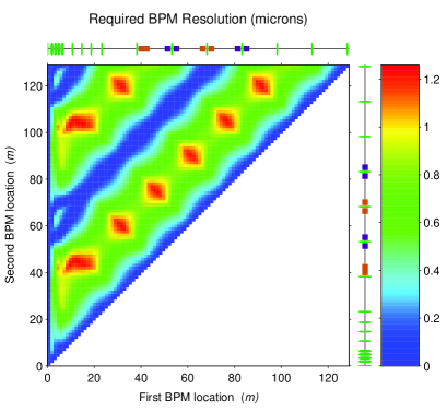
Figure 1: Maximal allowed resolution of two feedback BPM’s as a function of their positioning in the beam line.

References

- [1]
- [2] T.Lohse and P.Emma, “Linear Fitting of BPM Orbits and Lattice Parameters”, SLAC-CN-371 (1989).
- [3] Y.Chao, “Optics Measurement Resolution and BPM Errors”, Proc. PAC 1997, Vancouver, B.C., Canada, p.2125.
- [4] V.Balandin, W.Decking and N.Golubeva, “Errors in Reconstruction of Difference Orbit Parameters due to Finite BPM-Resolutions”, TESLA-FEL 2009-07, DESY, July 2009.
- [5] V.Balandin, W.Decking and N.Golubeva, “Errors in Measuring Transverse and Energy Jitter by Beam Position Monitors”, DESY 10-023, February 2010.
- [6] M.Altarelli, R.Brinkmann et al. (Eds), “XFEL: The European X-Ray Free-Electron Laser. Technical Design Report”, DESY 2006-097, DESY, Hamburg, 2006.
- [7] V.Balandin, W.Decking and N.Golubeva, “Magnet Lattice for High-Energy XFEL IBFB: Version of May 2008”, Unpublished Note.