More than one Author with different Affiliations

Somoclu: An Efficient Parallel Library for Self-Organizing Maps

Abstract

Somoclu is a massively parallel tool for training self-organizing maps on large data sets written in C++. It builds on OpenMP for multicore execution, and on MPI for distributing the workload across the nodes in a cluster. It is also able to boost training by using CUDA if graphics processing units are available. A sparse kernel is included, which is useful for high-dimensional but sparse data, such as the vector spaces common in text mining workflows. Python, R and MATLAB interfaces facilitate interactive use. Apart from fast execution, memory use is highly optimized, enabling training large emergent maps even on a single computer.

1 Introduction

Visual inspection of data is crucial to gain an intuition of the underlying structures. As data often lies in a high-dimensional space, we use embedding techniques to reduce the number of dimensions to just two or three.

Methods that rely on eigenvalue decomposition, such as multidimensional scaling [4], achieve a global optimum for such an embedding: The global topology of the space will be preserved.

Often the data points lie on a high-dimensional manifold that is curved and nonlinear. These structures are difficult to find with eigenvalue decomposition. Manifold learning generalizes embedding further, assuming that data in a high-dimensional space aligns to a manifold in a much lower dimensional space. For example, the algorithm Isomap finds a globally optimal solution for an underlying nonlinear manifold and it builds on multidimensional scaling [21]. Isomap, however, fails to find nonconvex embeddings [28].

Nonconvex structures are one strong motivation to look at solutions that are not globally optimal, but preserve the local topology of the space instead. Self-organizing maps (SOMs) are a widespread visualization tool that embed high-dimensional data on a two-dimensional surface – typically a section of a plane or a torus – while preserving the local topological layout of the original data [10]. These maps provide a visual representation of groups of similar data instances, and they are also useful in analyzing the dynamics of evolving data collections, as updates are easily made. Emergent self-organizing maps contain a much larger number of target nodes for embedding, and thus capture the topology of the original space more accurately [24].

Training a map is computationally demanding, but a great advantage of SOMs is that the computations are easy to parallelize. They have been accelerated on massively parallel graphics processing units (GPUs [14]). Tools exist that scale to large data sets using cluster resources [20], and also combining GPU-accelerated nodes in clusters [29]. These tools focus on batch processing. On the other end of the spectrum, interactive environments for training SOMs are often single-core implementations [24], not making full use of contemporary hardware.

We develop a common computational core that is highly efficient with the available resources. This common core is used for a command-line interface to enable batch processing on cluster resources, but the same core is used as the computational back-end for environments popular in data analysis. The tool, named Somoclu (originally standing for SOM on a cluster), has the following improvements over other implementations:

• It is highly efficient in single-node multicore execution.

• Memory use is reduced by up to 50 per cent.

• Large emergent maps are feasible.

• A kernel for sparse data is introduced to facilitate text mining applications.

• Training time is reduced by graphics processing units when available.

• It improves the efficiency of distributing the workload across multiple nodes when run on a cluster.

• An extensive command-line interface is available for batch processing.

• Python [25], R [17] and MATLAB [22] interfaces facilitate interactive processing.

• Compatibility with Databionic ESOM Tools [24] ensures easy visualization.

The source code is available under GNU Public License Version 3 (http://peterwittek.github.io/Somoclu/). The Python version is also listed in the Python package index (https://pypi.python.org/pypi/Somoclu/). The R version is available from the Comprehensive R Archive Network (CRAN) at https://CRAN.R-project.org/package=RSomoclu/.

2 Self-organizing maps in batch mode

The SOM training algorithm constructs a nonlinear topology preserving mapping of the input data set $X=\{x(t)|t\in\{t_{0,\ldots,t_{f}}\}\}$, where $t_{0}$ and $t_{f}$ are the beginning and the end of the current training session, onto a set of neurons $M=\{n_{1},\ldots,n_{k}\}$ of a neural network [10]. The neurons of the network are arranged in a grid, with associated weight vectors

$$W=\{w_{1}(t),\ldots,w_{k}(t)\}$$ (1)

at a given time step $t$. $W$ is known as the code book.

Each data point $x(t)$ is mapped to its best matching unit

$$\mathrm{bm}(x(t))=n_{b}\in M,$$ (2)

such that

$$d(x(t),w_{b}(t))\leq d(x(t),w_{j}(t))\quad\forall w_{j}(t)\in W,$$ (3)

where $d$ is the distance function on the data set in the feature space. The neurons are arranged on a two dimensional map: Each neuron $i$ has a two coordinates in a grid. Next the weight vector of the best match neuron and its neighbors are adjusted toward the input pattern using the following equation:

$$w_{j}(t+1)=w_{j}(t)+\alpha h_{bj}(t)(x(t)-w_{j}(t)),$$ (4)

where $0<\alpha<1$ is the learning factor, and $h_{bj}(t)$ is the neighborhood function that decreases for neurons further away from the best match neuron in grid coordinates. A frequently used neighborhood function is the Gaussian:

$$h_{bj}=\exp\left(\frac{-\|r_{b}-r_{j}\|}{\delta(t)}\right),$$ (5)

where $r_{b}$ and $r_{j}$ stand for the coordinates of the respective nodes. The width $\delta(t)$ decreases from iteration to iteration to narrow the area of influence.

The training is repeated on the same data set to increase the fit, a training cycle is called an epoch. Eventually, the neighborhood function decreases to an extent that training might stop. The time needed to train an SOM grows linearly with the data set size, and it grows linearly with the number of neurons in the SOM. SOM has a batch formulation of updating the weights, which is widely used in parallel implementations:

$$w_{j}(t_{f})=\frac{\sum_{t^{\prime}=t_{0}}^{t_{f}}h_{bj}(t^{\prime})x(t^{\prime})}{\sum_{t^{\prime}=t_{0}}^{t_{f}}h_{bj}(t^{\prime})}.$$ (6)

While not directly related to the training, it is worth mentioning the U-matrix associated with a SOM, which depicts the average Euclidean distance between the code book vectors of neighboring neurons. Let $N(j)$ denote the immediate neighbors of a node $j$. Then the height value of the U-matrix for a node $j$ is calculated as

$$U(j)=\frac{1}{|N(j)|}\sum_{i\in N(j)}d(w_{i},w_{j}).$$ (7)

The purpose of the U-matrix is to give a visual representation of the topology of the network.

There is no shortage of implementations of SOM training algorithms. It comes integrated in data mining suites such as RapidMiner [8]. Dedicated visualization and training tools also exist, such as the Databionic ESOM Tools [24]. Popular languages used in data analytics all have SOM modules, including MATLAB [26], Python [7], and R [27]. Common to these tools is that they seldom make use of parallel computing capabilities, although the batch formulation of SOM training invites such implementations. Further constraints include memory requirements, which increase fast with the size of the neuron grid.

Lower level libraries address such scalability issues. Distributing the workload across multiple nodes is feasible via standard methods such as MPI and MapReduce [11, 20]. The inherent parallelism is easy to exploit with graphics processing units (GPUs [14]). A method combining distributed computing with parallelism on GPUs is also available [29].

With Somoclu, we bridge high-level languages and massively parallel architectures, while also simplifying the distribution of workload compared to earlier implementations. We use a common core written in C++, supplemented by OpenMP [5], MPI [19], and CUDA [16]. This common core is used by an extensive command-line interface, and wrappers in Python, R, and MATLAB.

3 High-performance core for training

The starting point was a MapReduce-based distributed implementation of SOM [20]. This implementation was later accelerated by GPUs [29]. We found the MapReduce framework unnecessary, and derived a purely MPI-based implementation, that is more modular, faster, and includes a sparse kernel. Design details are provided in Section 3.1. Distributing the workload across multiple nodes is an extension of the parallel formulation (Section 3.2).

3.1 Parallelism

The dense CPU kernel is a straightforward implementation of the batch formulation in Equation 6, and it resembles the one implemented by Ref. [20]. For an overview of the parallel organization, refer to Figure 1. The MapReduce calls were replaced by MPI functions, leading to a more streamlined code. Furthermore, single-node parallelism on multicore CPUs is redesigned to use OpenMP instead of MPI. This strategy avoids duplicating the code book: Each MPI process must have a copy of the code book, but OpenMP threads can work on the same copy. The simplification leads to a minimum fifty per cent reduction in memory even when only two threads are used.

A performance bottleneck in the original implementation was the accumulation of local weights into a new global code book by one single process on the master node. This is parallelized by an OpenMP directive. Furthermore, the influence radius $\delta(t)$ of a best matching node is thresholded, which translates to speed improvements without compromising the quality of the trained map.

The GPU variant is more complex compared to the CPU kernel. The complexity stems from the way the distance function is evaluated between the nodes of the SOM and the training data. To maximize parallelism, the Gram matrix is calculated, that is, a matrix of the distances between every data instance and the nodes of the SOM. A naïve approach would be to extend an efficient matrix multiplication algorithm, replacing the dot product by the distance function. Opting for a Euclidean distance, it is possible to derive an alternative formulation of calculating the Gram matrix using linear algebra operations [13]. Benchmarking the two approaches, we found that the latter approach is a magnitude faster on the GPU, mainly due to a more favorable memory access pattern.

Figure 1: Overview of the parallel organization of the batch training. The global code book is replicated in each process, therefore it is more efficient to use OpenMP-based parallelization than to rely on MPI on multicore CPUs. If a GPU is available, it will overtake most data parallel operations from the CPU, replacing OpenMP threads.

We implemented the GPU kernel with Thrust [2], a C++ template library for CUDA, which has high-performance primitives, avoiding the need to manually tune individual GPU calls. Compared to the implementation by Ref. [29], the device memory use of the GPU code is reduced to approximately one-third, and the new implementation completely avoids costly matrix transposing operations.

Further complexity arises from the disparity between the number of GPUs and the number of cores in a computer. The CPU kernel achieves maximum speed by running an MPI process on each available core, resulting in a far lower number of data instances per core and a speedier local update of the weights. For instance, if there are eight cores and two GPUs, than each GPU has four times more data to process and its corresponding MPI thread would have four times more data to update the local weights. While the GPU handles the load efficiently, it would be highly inefficient to use a single thread to update the local weights. We thus hybridized the kernel and rely on OpenMP to parallelize the weight update. The GPU implementation runs as many MPI processes on a node as there are GPUs, and uses all CPU cores in the weight update.

The sparse kernel is a straightforward extension of the dense CPU kernel, and its main virtue is the reduced memory use. A vector space coming from a text processing pipeline typically contains 1–5% nonzero elements, leading to a 20–100$\times$ reduction in memory use when using a sparse representation. This kernel does not have a GPU implementation, as the irregular access patterns that are inevitable with sparse data structures are not efficient on streaming architectures.

3.2 Workload in distributed environment

The training procedure has a simple communication structure in a distributed memory system. Finding the best matching unit in Equation 2 is independent for every data instance, resembling the parallel version. This means that we can distribute equally sized parts of the data to each node, without any further communication of training data later on.

The update of the code book requires two way communication between a master node and the slave nodes. Once all weight updates are calculated in a slave node, the local updates are sent to the master node, which accumulates the changes to the code book. The new code book is broadcast to all slave nodes.

This communication structure ensures a near-linear scaling for smaller code books. Emergent maps with high-dimensional data, however, scale poorly. The code book is always a dense structure, even if the training data is sparse, as there are hardly any zero entries. Storing the code book in memory is the primary constraint for single node execution, and it is also the key constraint in distributed workloads.

Compared to an earlier GPU-accelerated, distributed implementation of SOM [29] that used MapReduce, we found that ordinary MPI calls are sufficient. Execution time did not improve significantly, but the overall code simplified, and our implementation does not have to rely on a little-used, MPI-based MapReduce library.

4 Interfaces

We regard the package libsvm for training support vector machines as a role model: Using an efficient computational core, numerous wrappers were added to the library to interface with other languages and environments [3]. The package fastcluster is also similar in its approach [15].

We provide an extensive command-line interface, which is able to access all functionality provided by the computational core (Section 4.1). The training functionality is exposed via an application programming interface, a single function that performs one epoch of training (Section 4.2). This function is wrapped to be called from Python, R, and MATLAB without duplicating data structures (Section 4.3).

4.1 Command-line interface

One sparse and two dense data formats are supported. All of them are plain text files. The entries can be separated by any white-space character. One row represents one data instance across all formats. Comment lines starting with a hash mark are ignored.

The basic dense format includes the coordinates of the data vectors, separated by a white-space. This file is parsed twice to get the basic dimensions right. The second dense format is identical, but it includes a header that contains information about the layout of the matrix. This second format is compatible with Databionic ESOM Tools.

The sparse representation is similarly row-oriented, and it uses the same sparse format as libsvm [3]. For instance, the vector [1.2 0 0 3.4] is represented as the following line in the file: 0:1.2 3:3.4. The file is parsed twice: once to get the number of instances and features, and the second time to read the data in the individual threads.

Example files are available in the package. Extension to further matrix types is simple to add.

The tool is used via the command line. Somoclu takes a plain text input file – either dense or sparse data. The basic execution is as follows:

$ [mpirun -np NPROC] Somoclu [OPTIONs] INPUT_FILE OUTPUT_PREFIX

The mpirun is required only when multiple nodes are used, or when there is more than one GPU in the system. The parameter INPUT_FILE is self-explanatory. Instead of names of output files for the best matching units, code books, and U-matrices, an output prefix is requested in OUTPUT_PREFIX. The resulting files will be differentiated by the extension, and, if interim snapshots are requested, also by the indices of the epochs in which the snapshots are taken.

The rest of the arguments are as follows.

-c FILENAME

The parameter specifies an initial code book for the map. The default is random initialization.

-e NUMBER

The number of training epochs, that is, the number of times each data instances will be presented to the learner.

-g TYPE

The type of the grid type; the default is square and the other option is hexagonal.

-k NUMBER

This parameter defines the kernel type. The value 0 stands for the dense CPU kernel, 1 is for the dense GPU kernel, and 2 is for the sparse CPU kernel.

-m TYPE

The map type is either planar or toroid; the default is planar.

-n FUNCTION

This option chooses the neighborhood function, which can be Gaussian or bubble; the default being the former.

-p NUMBER

If the neighborhood function is Gaussian, setting this parameter to 1 will cut off the update of nodes beyond the current radius.

-t STRATEGY

Radius cooling strategy is either linear or exponential; the default is linear.

-r NUMBER

The parameter defines the start radius. The default value is half of the map size in the smaller direction.

-R NUMBER

The final radius; it defaults to 1.

-T STRATEGY

Learning rate cooling strategy is either linear or exponential; the default is linear.

-l NUMBER

The starting learning rate; with a default value of 1.0.

-L NUMBER

The final learning rate; the default is 0.01.

-s NUMBER

This parameter decides whether to save interim files. The default value is 0, which means that no interim files will be saved. Setting the parameter to 1 will calculate and save the U-matrix in each time step. If the value passed is 2, then the code book and the best matching units are also saved in each epoch. Since the code book is enormous for large emergent maps, passing a value of 2 may significantly slow down each epoch.

-x, --columns NUMBER

This is the number of columns in map, that is, the size of the SOM in direction $x$; the default value is 50.

-y, --rows    NUMBER

The number of rows in map is defined by this value, that is, the size of the SOM in direction $y$; the default value is 50. Examples:

$ Somoclu data/rgbs.txt data/rgbs
$ mpirun -np 4 --hostfile hostfilename Somoclu -k 0 --rows 20 --columns 20 \
>   data/rgbs.txt data/rgbs

4.2 As an application programming interface

Designed to work with MPI, Somoclu was not conceived to be used as an API. Yet, given sufficient preparation on the calling side, it is possible to interface with Somoclu as an API. The primary entry point for training is the following function, as specified in Somoclu.h:

void trainOneEpoch(int itask, float *data, svm_node **sparseData,
  float *codebook, int *globalBmus, unsigned int nEpoch,
  unsigned int currentEpoch, unsigned int nSomX, unsigned int nSomY,
  unsigned int nDimensions, unsigned int nVectors,
  unsigned int nVectorsPerRank, unsigned int radius0,
  unsigned int radiusN, string radiusCooling, float scale0, float scaleN,
  string scaleCooling, unsigned int kernelType, string mapType,
  string gridType, bool compact_support, bool gaussian)

The parameters nSomX, nSomY, nEpoch, kernelType, and so on, are self-explanatory, they are the same as in the command-line interface.

The parameter itask specifies the rank of the current MPI process. If the calling environment does not use MPI, the value should be set as zero.

Data are either stored in data or sparseData, depending on whether the data are dense or sparse. Only data belonging to the process is expected, not the full matrix. The parameter nVectors stores the total number of instances, whereas nVectorsPerRank the number of instances belonging to one MPI thread.

4.3 Python, R and MATLAB interfaces

Solutions for scalable data processing in higher level languages tend to be ad hoc. Focusing on R as an example, the R Installation and Administration manual states that the language is ill-suited for working with data structures larger than about 10–20% of the main memory [18]. The key problem is with the overheads on the data structures. Parallel processing is scarcely addressed. Some modules aim to overcome these barriers [9].

Distributed computing is also challenging for such languages. Most solutions work entirely on a case by case basis, such as the distributed text mining module for R [23].

The aim of the interfaces is to address the problem of memory use and parallel execution. The Python package easily installable from the Python package index. The R package is available from CRAN. These packaged variants rely on the OpenMP parallelism alone. To get the massive CUDA parallelism through the interfaces, users with basic software building knowledge can easily follow the instructions on the project site. MATLAB users need to follow the instructions on the project site to build the module as no central package distribution site is available. Distributed workloads directed from a high-level language remain for future development.

Starting with the Python interface, our primary concern is to avoid memory copies and duplicating large structures in memory. The native variable system of Python is not strictly typed, hence we require the use of numpy. Using numpy float32 data type for storing arrays, we map directly to the single-precision floats used in the C++ code. We pass pointers between the two languages, making the best use of memory and almost zero computational overhead. This interface encapsulates the training routines in a class to simplify the workflow.

An example use of the interface is as follows:

>>> import Somoclu
>>> import numpy
>>> data = numpy.loadtxt(’data/random.dat’)
>>> n_rows, n_columns = 50, 50
>>> som = Somoclu.Somoclu(n_columns, n_rows, data = data)
>>> som.train()

The final code book is in the class variable Somoclu.codebook, the best matching units are in Somoclu.bmus, and the U-matrix is also calculated in Somoclu.umatrix.

The R interface uses the Rcpp package to cast pointers and provide type conversions between R and C++ [6]. Since R uses double precision matrices by default, and Somoclu uses single-precision floats internally, we must convert between double and float arrays of the input and output. This makes the interface less efficient than the Python version. The interface integrates with the popular R SOM package kohonen to facilitate use. The following is an example on how to call the wrapper function from R:

R> library("RSomoclu")
R> data("rgbs", package = "RSomoclu")
R> input_data <- data.matrix(rgbs)
R> nSomX <- 50; nSomY <- 50
R> nEpoch <- 10
R> radius0 <- 0; radiusN <- 0
R> radiusCooling <- "linear"
R> scale0 <- 0; scaleN <- 0.01
R> scaleCooling <- "linear"
R> kernelType <- 0
R> mapType <- "planar"
R> res <- RSomoclu.train(input_data, nEpoch, nSomX, nSomY, radius0, radiusN,
+    radiusCooling, scale0, scaleN, scaleCooling, kernelType, mapType)

The code book is returned in res$codebook, the best matching units are in res$globalBmus, and the calculated final U-matrix is in res$uMatrix. Most R users will probably want to work with the map through the package kohonen:

R> sommap <- RSomoclu.kohonen(input_data, res)

The MATLAB interface uses the official MEX-file mechanism to interface with C++. As with R, MATLAB also defaults to double precision variables, rendering some overhead of type conversion inevitable. We designed a similar training function call to that of the SOM Toolbox [26]. And provided examples on visualization using both SOM Toolbox and Databionic ESOM Tools. The following is an example call from the MATLAB interface.

>> data = importdata(’data/random.dat’);
>> msize = [50 50];
>> sMap  = som_randinit(D, ’msize’, msize);
>> nEpoch = 10;
>> radius0 = 0;
>> radiusN = 0;
>> radiusCooling = ’linear’;
>> scale0 = 0;
>> scaleN = 0.01;
>> scaleCooling = ’linear’;
>> kernelType = 0;
>> mapType = ’planar’;
>> gridType = ’rectangular’;
>> compactSupport = false;
>> neighborhood = ’gaussian’;
>> [sMap, sTrain, globalBmus, uMatrix] = ...
  Somoclu_train(sMap, data, ’msize’, msize, ’radius0’, radius0, ...
  ’radiusN’, radiusN, ’radiusCooling’, radiusCooling, ...
  ’scale0’, scale0, ’scaleN’, scaleN, ’scaleCooling’, scaleCooling, ...
  ’kernelType’, kernelType, ’mapType’, mapType, ...
  ’gridType’, gridType, ’compactSupport’, compactSupport, ...
  ’neighborhood’, neighborhood, ’nEpoch’, nEpoch);

The returned variables are identical to the Python version.

4.4 Visualization

The primary purpose of generating a map is visualization. Yet – apart from the Python interface – Somoclu does not come with its own functions for visualization, since there are countless generic and SOM-specific tools that are capable of plotting high-quality figures. The code book, the best matching units, and the U-matrix are exported at the end of the training, or even after each epoch.

The simplest procedure is to use a generic plotting library, such as gnuplot. For instance, the following simple gnuplot script plots the U-matrix in PNG format:

gnuplot> set datafile commentschars "#!%"
gnuplot> set autoscale
gnuplot> unset log
gnuplot> unset label
gnuplot> set lmargin at screen 0
gnuplot> set rmargin at screen 1
gnuplot> set bmargin at screen 0
gnuplot> set tmargin at screen 1
gnuplot> unset xtic
gnuplot> unset ytic
gnuplot> set notitle
gnuplot> set pm3d at b
gnuplot> set pm3d map
gnuplot> set nokey
gnuplot> set nocolorbox
gnuplot> unset surface
gnuplot> set term pngcairo transparent size 500,500
gnuplot> set output ’umatrix.png’
gnuplot> splot "filename"  matrix

The dimensions of the picture should be adapted to the size of the network to avoid distortion.

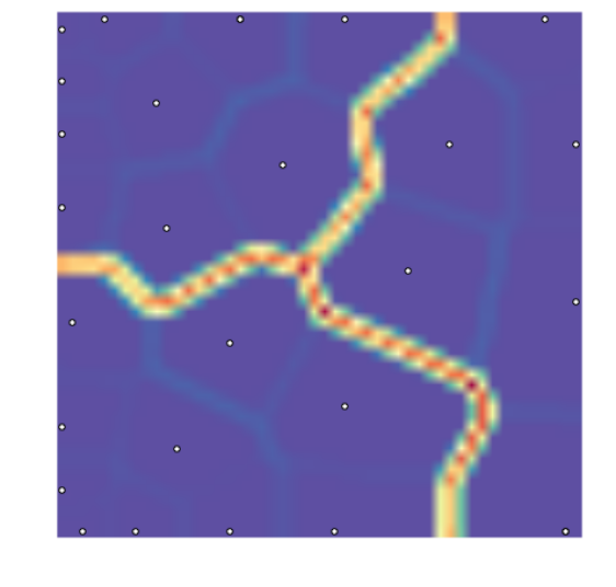
(a) The complete map.

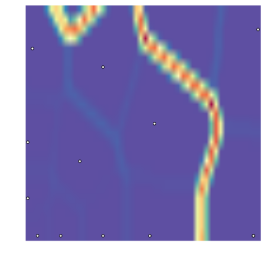
(b) A close-up of region.

Figure 2: The U-matrix of a toroid map with labels trained on a toy example plotted in Python.

The Python interface is equipped with plotting routines. For instance, a map can be plotted along with the labels or class colors:

>>> som.view_umatrix(bestmatches = True)

We may also zoom in to a specific part of the map:

>>> som.view_umatrix(bestmatches = True, zoom = ((n_rows//2, n_rows), (0, n_columns)))

Using a toy example included with the code, we obtained a visualization shown in Figure 2.

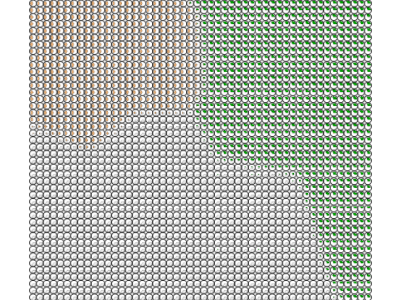
(a) Codebook.

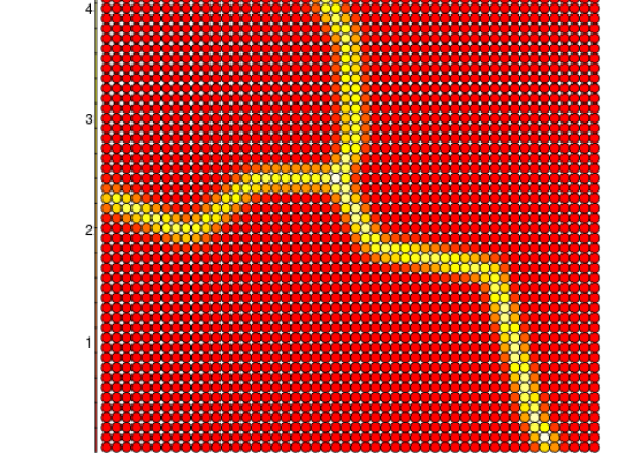
(b) U-matrix.

Figure 3: Visualizing a toy example trained by Somoclu and plotted by kohonen in R.

The R interface allows visualization through the package kohonen. This is entirely external to the library. A conversion to kohonen’s format is necessary:

R> sommap <- RSomoclu.kohonen(input_data, res)
R> plot(sommap, type = "codes", main = "Codes"))
R> plot(sommap, type = "dist.neighbours")

A toy example is shown in Figure 3.

The results of the MATLAB interface allows visualization through the SOM Toolbox, which is also external to the library.

>> som_show(sMap);

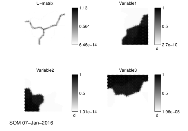
Figure 4: Visualizing a toy example trained by Somoclu and plotted by SOM Toolbox in MATLAB.

The toy example is shown Figure 4.

More advanced, SOM-specific tools may also offer an interactive GUI to select gradients and other parameters. One such tool is Databionic ESOM Tools [24], with which the output formats of Somoclu are compatible. The result of such visualization is shown in Section 5.3.

5 Experimental results

To ensure replicability of the results, we benchmarked with publicly available cluster GPU instances provided by Amazon Web Services. The instance type was cg1.4xlarge, equipped with 22 GiB of memory, two Intel Xeon X5570 quad-core CPUs, and two NVIDIA Tesla M2050 GPUs, running Ubuntu 12.04.

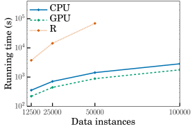
(a) $50{\times}50$ map.

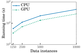
(b) $200{\times}200$ emergent map.

Figure 5: Training time on a single node with CPU and GPU kernels and the R package kohonen. The time axis is logarithmic. The data instances had 1,000 dimensions.

5.1 Single-node performance

The most direct comparison should be with the implementations by Refs. [20, 29]. Unfortunately the former was not able to handle the matrix sizes we were benchmarking with. The implementation by Ref. [29] is sensitive to the size of map, and it did not scale to the map sizes benchmarked here, and thus we left it out from the comparison. To compare with single-core performance, we included the R package kohonen [27]. The number of data instances ranged from 12,500 to 100,000, the number of dimensions was fixed at 1,000 for a regular $50\times 50$ self-organizing map. The data elements were randomly generated, as we were interested in scalability alone. We also tested an emergent map of $200\times{}200$ nodes, with the number of training instances ranging from 1,250 to 10,000. This large map size with the largest data matrix filled the memory of a single GPU, hence giving an upper limit to single-node experiments. Emergent maps in the package kohonen are not possible, as the map is initialized with a sample from the data instances. If the map has more nodes than data instances, kohonen exits with an error message. The map size did not affect the relative speed of the different kernels (Figure 5). The comparison was based on the command-line version of Somoclu.

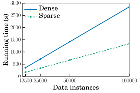
(a) Running time.

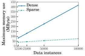
(b) Memory use.

Figure 6: Training time on a single node with dense and sparse kernels. The data instances had 1,000 dimensions, with five per cent of the elements being nonzero.

Compared to the R package, even the CPU version is at least ten times faster. The difference increases with the data size, indicating serious overhead problems in the R implementation.

The GPU results show at least a two-times speedup over the CPU version. This is less than expected, but this result considers a single GPU in the dual configuration, and the CPU is also a higher end model. These results, nevertheless, show that the Thrust template library is not efficient on two-dimensional data structures.

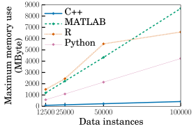
Figure 7: Memory overhead of the Python, R, and MATLAB interfaces compared to the command-line version (indicated as C++).

Comparing the sparse and dense kernels on a $50\times 50$ map, we benchmarked with random data instances of 1,000 dimensions that contained five per cent of nonzero elements (Figure 6). Execution time was about two times faster with the sparse kernel. The reduction in memory use was far more dramatic, the sparse kernel using only twenty per cent of the memory of the dense one with 100,000 instances. Naturally, the difference with emergent maps would be less apparent, as the code book is always stored in a dense format.

Measuring the memory overhead of the interfaces compared to the native version, we are not surprised to see that the Python variant is the closest (Figure 7). As the data structures are not duplicated in this interface, it is still counter-intuitive that the gap increases with larger data sets. The R and MATLAB versions have predictably larger and growing gaps compared to the command-line interface, as they both must duplicate all data structures. Apart from the time spent on duplicating the data structures in the R and MATLAB versions, the computational overhead is negligible in all interfaces.

5.2 Multi-node scaling

Using 100,000 instances and a map of $50\times 50$ nodes, the calculations scale in a linear fashion (Figure 8). This was expected, as there is little communication between nodes, apart from the weight updates. As calculations cannot overlap with communication, we did not benchmark the GPU kernel separately, as its scaling is identical to that of the CPU kernel.

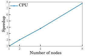
Figure 8: Speedup on multiple nodes with CPU kernel compared to a single node. The data instances had 1,000 dimensions.

5.3 Visualization on real data

We used the Reuters-21578 document collection for an example on text mining visualization [12]. We used Lucene 3.6.2 [1] to create an inverted index of the document collection. Terms were stemmed and we discarded those that occurred less than three times or were in the top ten per cent most frequent ones. Thus we had 12,347 index terms, lying in an approximately twenty-thousand dimensional space.

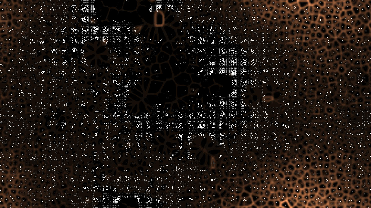
Figure 9: The U-matrix of a toroid emergent self-organizing map after ten epochs of training on the feature space of sparse data. The individual dots are neurons with a weight vector that match a data instance. The other neurons reflect the distances in the original high-dimensional space.

We trained a toroid emergent self-organizing map of $336\times 205$ dimensions. The initial learning rate was 1.0, which decreased linearly over ten epochs to 0.1. The initial radius for the neighborhood was a hundred neurons, and it also decreased linearly to one. The neighborhood function was a noncompact Gaussian.

We studied the U-matrix of the map. Visualizing this with the Databionic ESOM Tools [24], we plotted the global structure of the map in Figure 9. The map clearly shows dense areas where index terms are close and form tight clusters. Other parts of the map are sparse, with large barriers separating index terms into individual semantic regions.

6 Limitations

The most constraining limitation is the storing of the code book in the main memory. While memory use has been optimized, and only the number of computing nodes sets a limit to the amount of data to be processed, each node keeps a full copy of the code book. This is not a problem for feature spaces of a few thousand dimensions – even emergent maps are easy to compute. Yet, if the feature space has over tens of thousands or more features, emergent maps are no longer feasible.

Currently only the command-line interface is able to unlock all the capabilities of the computing core. The R, Python and MATLAB interfaces can use capabilities of the OpenMP and CUDA core, but these wrappers cannot use a distributed cluster for the calculations.

The R interface cannot support the GPU kernel easily on Windows due to incompatibilities between the R supported compiler GCC and the CUDA supported compiler Visual C++, while on Linux and OS X it can be built easily.

7 Conclusions

Do we need another implementation of self-organizing maps? We believe the answer is yes. Libraries in high-level languages do not have a scalable training module, and even implementations on parallel and distributed architectures could be improved on. Our solution scales from a single-thread execution to massively parallel GPU-accelerated clusters using a common core. Batch processing is encouraged by a command-line interface, whereas interactive use is enabled by Python, R, and MATLAB interfaces. Even when called interactively, execution is parallelized.

• Memory-efficient multicore execution.

• Purely MPI-based, highly efficient distributed implementation.

• Optimized hybrid CPU-GPU kernel for boosting training on dense data.

• Sparse kernel.

• Common computational back-end for popular data-processing languages: Python, R, and MATLAB.

• Windows, OS X, Linux support of the command-line interface, with full parallel capability.

• Highly efficient on large emergent maps.

• Format compatibility with ESOM Tools for visualization.

As emergent maps are especially computationally intensive, we believe that the primary usage scenario is a single-node, multi-GPU configuration for data exploration, which was only feasible for small maps and small volumes of data until now. Larger volumes of data are also easy to compute on a cluster.

References

- [1] Apache Software Foundation. Apache Lucene: Free and Open-Source Information Retrieval Software Library, 2012. Version 3.6.2.
- [2] Nathan Bell and Jared Hoberock. Thrust: A productivity-oriented library for CUDA. In GPU Computing Gems, volume 7. Morgan Kaufmann, 2011.
- [3] Chih-Chung Chang and Chih-Jen Lin. libsvm: A Library for Support Vector Machines, 2001.
- [4] Trevor F. Cox and Michael A.A. Cox. Multidimensional Scaling. Chapman and Hall, 1994.
- [5] Leonardo Dagum and Ramesh Menon. OpenMP: An industry standard API for shared-memory programming. Computational Science & Engineering, 5(1):46–55, 1998.
- [6] Dirk Eddelbuettel and Romain François. Rcpp: Seamless R and C++ integration. Journal of Statistical Software, 40(8):1–18, 2011.
- [7] Michael Hanke, Yaroslav O Halchenko, Per B Sederberg, Stephen José Hanson, James V Haxby, and Stefan Pollmann. PyMVPA: A Python toolbox for multivariate pattern analysis of fMRI data. Neuroinformatics, 7(1):37–53, 2009.
- [8] Markus Hofmann and Ralf Klinkenberg. RapidMiner: Data Mining Use Cases and Business Analytics Applications. Chapman and Hall, 2013.
- [9] Michael Kane, John W. Emerson, and Stephen Weston. Scalable strategies for computing with massive data. Journal of Statistical Software, 55(14):1–19, 2013.
- [10] Teuvo Kohonen. Self-Organizing Maps. Springer-Verlag, 2001.
- [11] Richard D. Lawrence, George S. Almasi, and Holly E. Rushmeier. A scalable parallel algorithm for self-organizing maps with applications to sparse data mining problems. Data Mining and Knowledge Discovery, 3(2):171–195, 1999.
- [12] David D. Lewis. Reuters-21578 text categorization test collection distribution 1.0, 1999.
- [13] Qi Li, Vojislav Kecman, and Raied Salman. A chunking method for Euclidean distance matrix calculation on large dataset using multi-GPU. In Proceedings of ICMLA-10, 9th International Conference on Machine Learning and Applications, pages 208–213, Washington, DC, USA, 2010.
- [14] Zhongwen Luo, Hongzhi Liu, Zhengping Yang, and Xincai Wu. Self-organizing maps computing on graphic process unit. In Proceedings of ESANN-05, 13th European Symposium on Artificial Neural Networks, 2005.
- [15] Daniel Müllner. fastcluster: Fast hierarchical, agglomerative clustering routines for R and Python. Journal of Statistical Software, 53(9):1–18, 2013.
- [16] NVidia Corporation. NVida Compute Unified Device Architecture Programming Guide 6.0, 2014.
- [17] R Core Team. R: A Language and Environment for Statistical Computing. R Foundation for Statistical Computing, Vienna, Austria, 2017.
- [18] R Core Team. R Installation and Administration. R Foundation for Statistical Computing, Vienna, Austria, 2017.
- [19] Marc Snir, Steve W. Otto, Steven Huss-Lederman, David W. Walker, and Jack Dongarra. MPI – The Complete Reference: The MPI Core, volume 1. MIT Press, 1998.
- [20] Seung-Jin Sul and Andrey Tovchigrechko. Parallelizing BLAST and SOM algorithms with mapreduce-mpi library. In Proceedings of IPDPS-11, 25th International Parallel and Distributed Computing Symposium, pages 476–483, Anchorage, AK, USA, 2011.
- [21] Joshua B. Tenenbaum, Vin de Silva, and John C. Langford. A global geometric framework for nonlinear dimensionality reduction. Science, 290(5500):2319–2323, 2000.
- [22] The MathWorks Inc. MATLAB: The language of technical computing, version R2011b, 2011.
- [23] Stefan Theußl, Ingo Feinerer, and Kurt Hornik. A tm plug-in for distributed text mining in R. Journal of Statistical Software, 51(5):1–31, 2012.
- [24] Alfred Ultsch and Fabian Mörchen. ESOM-Maps: Tools for clustering, visualization, and classification with emergent SOM. Technical report, Data Bionics Research Group, University of Marburg, 2005.
- [25] Guido van Rossum. Python Programming Language, 2014.
- [26] Juha Vesanto, Johan Himberg, Esa Alhoniemi, and Juha Parhankangas. Self-organizing map in MATLAB: The SOM Toolbox. Proceedings of the MATLAB DSP Conference, pages 35–40, 1999.
- [27] Ron Wehrens and Lutgarde M. C. Buydens. Self- and super-organizing maps in R: The kohonen package. Journal of Statistical Software, 21(5):1–19, 2007.
- [28] Kilian Q. Weinberger, Fei Sha, and Lawrence K. Saul. Learning a kernel matrix for nonlinear dimensionality reduction. In Proceedings of ICML-04, 21st International Conference on Machine Learning, pages 106–113, Banff, Canada, 2004.
- [29] Peter Wittek and Sándor Darányi. A GPU-accelerated algorithm for self-organizing maps in a distributed environment. In Proceedings of ESANN-12, 20th European Symposium on Artificial Neural Networks, Computational Intelligence and Machine Learning, Bruges, Belgium, 2012.