Comb-like models for transport along spiny dendrites

Abstract

We suggest a modification of a comb model to describe anomalous transport in spiny dendrites. Geometry of the comb structure consisting of a one-dimensional backbone and lateral branches makes it possible to describe anomalous diffusion, where dynamics inside fingers corresponds to spines, while the backbone describes diffusion along dendrites. The presented analysis establishes that the fractional dynamics in spiny dendrites is controlled by fractal geometry of the comb structure and fractional kinetics inside the spines. Our results show that the transport along spiny dendrites is subdiffusive and depends on the density of spines in agreement with recent experiments.

1 Introduction

Dendritic spines are small protrusions from many types of neurons located on the surface of a neuronal dendrite. They receive most of the excitatory inputs and their physiological role is still unclear although most spines are thought to be key elements in neuronal information processing and plasticity [1]. Spines are composed of a head ($\sim 1$ $\mu$m) and a thin neck ($\sim 0.1$ $\mu$m) attached to the surface of dendrite (see Fig. 1). The heads of spines have an active membrane, and as a consequence, they can sustain the propagation of an action potential with a rate that depends on the spatial density of spines [2]. Decreased spine density can result in cognitive disorders, such as autism, mental retardation and fragile X syndrome [3]. Diffusion over branched smooth dendritic trees is basically determined by classical diffusion and the mean square displacement (MSD) along the dendritic axis grows linearly with time. However, inert particles diffusing along dendrites enter spines and remain there, trapped inside the spine head and then escape through a narrow neck to continue their diffusion along the dendritic axis. Recent experiments together with numerical simulations have shown that the transport of inert particles along spiny dendrites of Purkinje and Piramidal cells is anomalous with an anomalous exponent that depends on the density of spines [4, 5, 6]. Based on these results, a fractional Nernst-Planck equation and fractional cable equation have been proposed for electrodiffusion of ions in spiny dendrites [7]. Whereas many studies have been focused to the coupling between spines and dendrites, they are either phenomenological cable theories [7, 8] or microscopic models for a single spine and parent dendrite [9, 10]. More recently a mesoscopic non-Markovian model for spines-dendrite interaction and an extension including reactions in spines and variable residence time have been developed [11, 12]. These models predict anomalous diffusion along the dendrite in agreement with the experiments but are not able to relate how the anomalous exponent depends on the density of spines [5, 6]. Since these experiments have been performed with inert particles (i.e., there are not reaction inside spines or dendrites) we conclude that the observed anomalous diffusion is due exclusively to the geometric structure of the spiny dendrite. Recent studies on the transport of particles inside spiny dendrites indicate the strong relation between the geometrical structure and anomalous transport exponents [5, 13, 14]. Therefore, elaboration such an analytical model that establishes this relation can be helpful for further understanding transport properties in spiny dendrites. The real distribution of spines along the dendrite, their size and shapes are completely random [3], and inside spines the spine necks act as a transport barrier [9]. For these reasons we reasonably assume that the diffusion inside spine is anomalous. So, we propose in this paper models based on a comb-like structure that mimic a spiny dendrite; where the backbone is the dendrite and the fingers (lateral branches) are the spines. The models predict anomalous transport inside spiny dendrites, in agreement with the experimental results of Ref. [4], and also explain the dependence between the mean square displacement and the density of spines observed in [5].

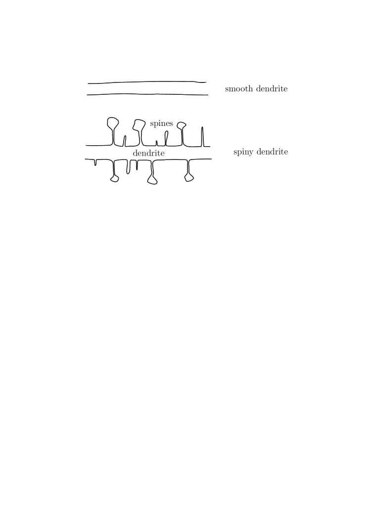
Figure 1: Schematic drawing of smooth and spiny dendrites.

2 Model I: Anomalous diffusion in spines

Geometry of the comb structure consisting of a one-dimensional backbone and lateral branches (fingers) [15] makes it possible to describe anomalous diffusion in spiny dendrites structure in the framework of the comb model. In this case dynamics inside fingers corresponds to spines, while the backbone describes diffusion inside dendrites. The comb model is an analogue of a 1D medium where fractional diffusion has been observed and explained in the framework of a so-called continuous time random walk [15, 16, 17, 18].

Usually, anomalous diffusion on the comb is described by the $2D$ distribution function $P=P(x,y,t)$, and a special behavior is that the displacement in the $x$–direction is possible only along the structure backbone ($x$-axis at $y=0$). Therefore, diffusion in the $x$-direction is highly inhomogeneous. Namely, the diffusion coefficient is $D_{xx}=D_{x}\delta(y)$, while the diffusion coefficient in the $y$–direction (along fingers) is a constant $D_{yy}=D_{y}$. Due to this geometrical construction, the flux of particles along the dendrite is

$$J_{x}=-D_{x}\delta(y)\frac{\partial P}{\partial x}$$ (1)

and the flux along the finger describes the anomalous trapping process that occurs inside the spine

$$J_{y}=\left.-D_{y}\frac{\partial^{1-\gamma}}{\partial t^{1-\gamma}}\right|_{RL}\frac{\partial P}{\partial y}$$ (2)

where $P(x,y,t)$ is the density of particles and

$$\left.\frac{\partial^{1-\gamma}}{\partial t^{1-\gamma}}\right|_{RL}f(t)=\frac{\partial}{\partial t}I_{t}^{\gamma}f(t)$$ (3)

is the Riemann-Liouville fractional derivative, where the fractional integration $I_{t}^{\gamma}$ is defined by means of the Laplace transform

$$\hat{\mathcal{L}}\left[I_{t}^{\gamma}f(t)\right]=s^{-\gamma}\tilde{f}(s)\,.$$ (4)

So, inside the spine, the transport process is anomalous and $\left\langle y^{2}(t)\right\rangle\sim t^{\gamma}$, where $\gamma\in(0,1)$. Making use of the continuity equation for the total number of particles

$$\frac{\partial P}{\partial t}+\mbox{div}\mathbf{J}=0\,,$$ (5)

where $\mathbf{J}=(J_{x},J_{y})$ one has the following evolution equation for transport along the spiny dendrite

$$\frac{\partial P}{\partial t}-D_{x}\delta(y)\frac{\partial^{2}P}{\partial x^{2}}-D_{y}\frac{\partial^{1-\gamma}}{\partial t^{1-\gamma}}\Big{|}_{RL}\frac{\partial^{2}P}{\partial y^{2}}=0.$$ (6)

The Riemann-Liouville fractional derivative in Eq. (6) is not convenient for the Laplace transform. To ensure feasibility of the Laplace transform, which is a strong machinery for treating fractional equations, one reformulates the problem in a form suitable for the Laplace transform application.

To shed light on this situation, let us consider a comb in the $3D$ [19]. This model is described by the distribution function $P_{1}(x,y,z,t)$ with evolution equation given by the equation

$$\frac{\partial P_{1}}{\partial t}-D_{x}\delta(y)\delta(z)\frac{\partial^{2}P_{1}}{\partial x^{2}}-D_{y}\delta(z)\frac{\partial^{2}P_{1}}{\partial y^{2}}-\frac{\partial^{2}P_{1}}{\partial z^{2}}=0\,.$$ (7)

It should be stressed that $z$ coordinate is a supplementary, virtue variable, introduced to described fractional motion in spines by means of the Markovian process. Thus the true distribution is $P(x,y,t)=\int_{-\infty}^{\infty}P_{1}(x,y,z,t)dz$ with corresponding evolution equation

$$\frac{\partial P}{\partial t}-D_{x}\delta(y)\frac{\partial^{2}P_{1}(z=0)}{\partial x^{2}}-D_{y}\frac{\partial^{2}P_{1}(z=0)}{\partial y^{2}}=0\,.$$ (8)

A relation between $P(x,y,t)$ and $P_{1}(x,y,z=0,t)$ can be expressed through their Laplace transforms (see derivation in the Appendix)

$$\tilde{P}_{1}(x,y,z=0,s)=\frac{\sqrt{s}}{2}\tilde{P}(x,y,s)\,,$$ (9)

where $\tilde{P}(x,y,s)=\hat{\mathcal{L}}[P(x,y,t)]$ and $\tilde{P}_{1}(x,y,z,s)=\hat{\mathcal{L}}[P_{1}(x,y,z,t)]$. Therefore, performing the Laplace transform of Eq. (8) yields

$$s\tilde{P}(x,y,s)-D_{x}\delta(y)\frac{\partial^{2}\tilde{P}_{1}(x,y,z=0,s)}{\partial x^{2}}-D_{y}\frac{\partial^{2}\tilde{P}_{1}(x,y,z=0,s)}{\partial y^{2}}=P(x,y,t=0)$$ (10)

and substituting relation (9), dividing by $\sqrt{s}$ and then performing the Laplace inversion, one obtains the comb model with the fractional time comb model

$$\frac{\partial^{\frac{1}{2}}P}{\partial t^{\frac{1}{2}}}-D_{x}\delta(y)\frac{\partial^{2}P}{\partial x^{2}}-D_{y}\frac{\partial^{2}P}{\partial y^{2}}=0\,,$$ (11)

where $2D_{x,y}\rightarrow D_{x,y}$ and the Caputo derivative $\frac{\partial^{\gamma}}{\partial t^{\gamma}}$ can be defined by the Laplace transform for $\gamma\in(0,1)$ [20]

$$\hat{\mathcal{L}}\left[\frac{\partial^{\gamma}f}{\partial t^{\gamma}}\right]=s^{\gamma}\tilde{f}(s)-s^{\gamma-1}f(t=0)\,.$$ (12)

The fractional transport takes place in both the dendrite $x$ direction and the spines $y$ coordinate. To make fractional diffusion in dendrite normal, we add the fractional integration $I_{t}^{1-\gamma}$ by means of the Laplace transform (4), as well $\hat{\mathcal{L}}\left[I_{t}^{1-\gamma}f(t)\right]=s^{\gamma-1}\tilde{f}(s)$. This yields Eq. (11), after generalization $\frac{1}{2}\rightarrow\gamma\in(0,1)$,

$$\frac{\partial^{\gamma}P}{\partial t^{\gamma}}-D_{x}\delta(y)I_{t}^{1-\gamma}\frac{\partial^{2}P}{\partial x^{2}}-D_{y}\frac{\partial^{2}P}{\partial y^{2}}=0.$$ (13)

Performing the Fourier-Laplace transform in (13) we get

$$P(k_{x},k_{y},s)=\frac{P(k_{x},k_{y},t=0)-D_{x}k_{x}^{2}P(k_{x},y=0,s)}{s+D_{y}k_{y}^{2}s^{1-\gamma}}\,,$$ (14)

where the Fourier-Laplace image of the distribution function is defined by its arguments $\hat{\mathcal{L}}\hat{\mathcal{F}}_{x}\hat{\mathcal{F}}_{y}[P(x,y,t)]=P(k_{x},k_{y},s)$. If $P(x,y,t=0)=\delta(x)\delta(y)$, inversion by Fourier over $y$ gives

$$P(k_{x},y,s)=\frac{1-D_{x}k_{x}^{2}P(k_{x},y=0,s)}{s^{(2-\gamma)/2}\sqrt{D_{y}}}\exp\left(-\left|y\right|s^{\gamma/2}/\sqrt{D_{y}}\right).$$ (15)

Taking $y=0$ the above equation provides

$$P(k_{x},y=0,s)=\frac{1}{s^{(2-\gamma)/2}\sqrt{D_{y}}+D_{x}k_{x}^{2}}$$ (16)

which inserted into (14) yields

$$P(k_{x},k_{y},s)=\frac{1}{s+D_{y}k_{y}^{2}s^{1-\gamma}}\left(1-\frac{D_{x}k_{x}^{2}}{s^{(2-\gamma)/2}\sqrt{D_{y}}+D_{x}k_{x}^{2}}\right).$$ (17)

We can calculate the density of particles at a given point $x$ of the dendrite at time $t,$ namely $P(x,t),$ by integrating over $y$

$$P(k_{x},s)=P(k_{x},k_{y}=0,s)=\frac{s^{-\gamma/2}\sqrt{D_{y}}}{s^{(2-\gamma)/2}\sqrt{D_{y}}+D_{x}k_{x}^{2}},$$ (18)

then

$$\left\langle x^{2}(s)\right\rangle=-\left.\frac{\partial^{2}}{\partial k_{x}^{2}}P(k_{x},s)\right|_{k_{x}=0}=\frac{2D_{x}}{\sqrt{D_{y}}}\frac{1}{s^{2-\frac{\gamma}{2}}}$$ (19)

so that

$$\left\langle x^{2}(t)\right\rangle=\frac{2D_{x}}{\sqrt{D_{y}}}t^{1-\frac{\gamma}{2}}.$$ (20)

Eq. (20) predicts subdiffusion along the spiny dendrite which is in agreement with the experimental results reported in [4]. It should be noted that this result is counterintuitive. Indeed, subdiffusion in spines, or fingers should lead to the slower subdiffusion in dendrites, or backbone with the transport exponent less than in usual comb, since these two processes are strongly correlated. But this correlation is broken due to the fractional integration $I_{t}^{1-\gamma}$ in Eq. (13). On the other hand, if we invert (18) by Fourier-Laplace we obtain the fractional diffusion equation for $P(x,t)$

$$\frac{\partial^{1-\frac{\gamma}{2}}P}{\partial t^{1-\frac{\gamma}{2}}}=\frac{D_{x}}{\sqrt{D_{y}}}\frac{\partial^{2}P}{\partial x^{2}}$$

which is equivalent to the generalized Master equation

$$\frac{\partial P}{\partial t}=\int_{0}^{t}M(t-t^{\prime})\frac{\partial^{2}P(x,t^{\prime})}{\partial x^{2}}dt^{\prime}$$ (21)

if the Laplace transform of the memory kernel is given by $M(s)=\frac{D_{x}}{\sqrt{D_{y}}}s^{\gamma/2}$, which corresponds to the waiting time PDF in the Laplace space given by

$$\varphi(s)=\frac{1}{1+\frac{\sqrt{D_{y}}}{D_{x}}s^{1-\frac{\gamma}{2}}}$$ (22)

that is $\varphi(t)\sim t^{-2+\frac{\gamma}{2}}$ as $t\rightarrow\infty$. The above waiting time PDF is the effective PDF corresponding to the whole comb and takes into account the particle trapping inside spines. Let us employ the notation for a dynamical exponent $d_{w}$ used in [4, 5]. If $d_{w}=4/(2-\gamma)$ then the MSD grows as $t^{2/d_{w}}$. On the other hand, it has been found in experiments that $d_{w}$ increases with the density of spines $\rho_{s}$ and the simulations prove that $d_{w}$ grows linearly with $\rho_{s}$. Indeed, the experimental data admits almost any growing dependence of $d_{w}$ with $\rho_{s}$ due to the high variance of the data (see Fig 5.D in [5]). Equation (20) also establishes a phenomenological relation between the second moment and $\rho_{s}$. When the density spines is zero then $\gamma=0$, $d_{w}=2$ and normal diffusion takes place. If the spine density $\rho_{s}$ increases, the anomalous exponent of the PDF (22) $1-\gamma/2=2/d_{w}$ must decrease (i.e., the transport is more subdiffusive due to the increase of $\rho_{s}$) so that $d_{w}$ has to increase as well. So, our model predicts qualitatively that $d_{w}$ increases with $\rho_{s}$, in agreement with the experimental results in [5].

3 Model II: Lévy walks on fractal comb

In this section we consider a fractal comb model [21] to take into account the inhomogeneity of the spines distribution. The comb model is a phenomenological explanation of an experimental situation, where we introduce a control parameter that establishes a relation between diffusion along dendrites and the density of spines. Suggesting more sophisticated relation between the dynamical exponent and the spine density, we can reasonably suppose that the fractal dimension, due to the box counting of the spine necks, is not integer: it is embedded in the $1D$ space, thus the spine fractal dimension is $\nu\in(0,1)$. According the fractal geometry (roughly speaking), the most convenient parameter is the fractal dimension of the spine volume (mass) $\mu_{\rm spine}(x)\equiv\mu(x)\sim|x|^{\nu}$. Therefore, following Nigmatulin’s idea on a construction of a “memory kernel” on a Cantor set in the Fourier space $|k|^{1-\nu}$ [22] (and further developing in Refs. [23, 24, 25]), this leads to a convolution integral between the non-local density of spines and the probability distribution function $P(x,y,t)$ that can be expressed by means of the inverse Fourier transform [21] $\hat{\mathcal{F}}_{x}^{-1}\left[|k_{x}|^{1-\nu}P(k_{x},y,t)\right]$. Therefore, the starting mathematical point of the phenomenological consideration is the fractal comb model

$$\frac{\partial^{\gamma}P}{\partial t^{\gamma}}-D_{x}\delta(y)I_{t}^{1-\gamma}\frac{\partial^{2}P}{\partial x^{2}}-D_{y}\frac{\partial^{2}}{\partial y^{2}}\hat{\mathcal{F}}_{k_{x}}^{-1}\left[|k_{x}|^{1-\nu}P(k_{x},y,t)\right]=0\,.$$ (23)

Performing the same analysis in the Fourier-Laplace space, presented in previous section, then eq. (18) reads

$$P(k_{x},s)=P(k_{x},k_{y}=0,s)=\frac{s^{-\gamma/2}\sqrt{D_{y}}}{s^{(2-\gamma)/2}\sqrt{D_{y}}+D_{x}|k_{x}|^{\beta}}\,,$$ (24)

where $\beta=3/2+\nu/2$.

Contrary to the previous analysis expression (19) does not work any more, since superlinear motion is involved in the fractional kinetics. This leads to divergence of the second moment due to the Lévy flights. The latter are described by the distribution $\sim 1/|x|^{1+\beta}$, which is separated from the waiting time probability distribution $\varphi(t)$. To overcome this deficiency, we follow the analysis of the Lévy walks suggested in [26, 27]. Therefore, we consider our exact result in Eq. (24) as an approximation obtained from the joint distribution of the waiting times and the Lévy walks. Therefore, a cutoff of the Lévy flights is expected at $|x|=t$. This means that a particle moves at a constant velocity inside dendrites not all times, and this laminar motion is interrupted by localization inside spines distributed in space by the power law.

Performing the inverse Laplace transform, we obtain solution in the form of the Mittag-Leffler function [28]

$$P(k_{x},t)=\mathcal{E}_{1-\gamma/2}\left(-D|k|^{\beta}t^{1-\gamma/2}\right)\,,$$ (25)

where $D=\frac{D_{x}}{\sqrt{D_{y}}}$. For the asymptotic behavior $|k|\rightarrow 0$ the argument of the Mittag-Leffler function can be small. Note that in the vicinity of the cutoff $|x|=t$ this corresponds to the large $t$ ($|k|\sim\frac{1}{t}\ll 1$), Thus we have [28]

$$\mathcal{E}_{1-\gamma/2}\left(-D|k|^{\beta}t^{1-\gamma/2}\right)\approx\exp\left(-\frac{D|k|^{\beta}t^{1-\gamma/2}}{\Gamma(2-\gamma/2)}\right)\,.$$ (26)

Therefore, the inverse Fourier transform yields

$$P(x,t)\approx A_{\gamma,\nu}\frac{Dt^{1-\gamma/2}}{\Gamma(2-\gamma/2)|x|^{(5+\nu)/2}}\,,$$ (27)

where $A_{\gamma,\nu}$ is determined from the normalization condition. Now the second moment corresponds to integration with the cutoff at $x=t$ that yields

$$\left\langle x^{2}(t)\right\rangle=K_{\gamma,\nu}t^{\frac{3-\gamma-\nu}{2}}\,,$$ (28)

where $K_{\gamma,\nu}=\frac{4A_{\gamma,\nu}D_{x}}{(1-\nu)\Gamma(2-\gamma/2)\sqrt{D_{y}}}$ is a generalized diffusion coefficient. Transition to absence of spines means first transition to normal diffusion in fingers with $\gamma=1$ and then $\nu=0$ that yields

$$\left\langle x^{2}(t)\right\rangle=K_{1,0}t\,.$$ (29)

4 Discussion

The present analysis establishes that the fractional dynamics in spiny dendrites can be described by two parameters, related to the fractal geometry of spines $\nu$ and fractional kinetics inside the spines $\gamma$. Summarizing, the most general phenomenological description can be performed in the framework of the fractional Fokker-Planck equation (FFPE)

$$\frac{\partial^{\alpha}P}{\partial t^{\alpha}}=K_{\alpha,\beta}\frac{\partial^{\beta}P}{\partial|x|^{\beta}}\,,$$ (30)

where, for the present analysis $\alpha=(2-\gamma)/2$ and $\beta=(3+\nu)/2$; in general case $\alpha\in(0,1)$ and $\beta\in(1,2)$ are arbitrary.

For $\beta=2$, we arrive at the first model, presented in Sec. II, where we deal with a one temporal control parameter $\gamma$ only. In this case, anomalous transport in dendrites, described by the dynamical exponent $d_{w}$, is characterized by anomalous transport inside spines, described by the transport exponent $\gamma$. The obtained relation $d_{w}=\frac{4}{2-\gamma}$ also establishes a relation between the dynamical exponent and the density of spines and is in agreement with recent experiments [4, 5, 6].

In the second model we suggested a more sophisticated relation between the dynamical exponent and the spine density. In this case $\beta=(3+\nu)/2<2$ depends on fractal dimension of spines, and this leads to an essential restriction for Eq. (30). The first one is a cutoff of the Lévy flights at $|x|=t$ that leads to a consequence of laminar and localized motions [27] and yields a finite second moment $\left\langle x^{2}(t)\right\rangle\sim t^{2+\alpha-\beta}$. When $\alpha=1/2$ and $\beta=2$ the FFPE (30) corresponds to the continuous comb model, namely spine dendrites with the maximal density of spines. For $\alpha=1/2$ and $\beta=3/2$ this model corresponds to smooth dendrites. Apparently, another physically sound transition to limiting case is possible for $\nu=1$ and $\gamma=0$ that corresponds first to the transition to the continuous model, and then the transition to $\gamma=0$. This physical control of the parameters ensures an absence of superdiffusion in Eq. (30). Another important question is what happens in intermediate cases. A challenging question here is what is the fractal dimension of the spine volume.

We conclude our consideration by presenting the physical reason of the possible power law distribution of the waiting time PDF $\varphi(t)$ in Eq. (22). At this point we paraphrase some arguments from Ref. [19] with the corresponding adaptation to the present analysis. Let us consider the escape from a spine cavity from a potential point of view, where geometrical parameters of the cavity can be related to a potential $U$. For example, let us consider spines with a head of volume $V$ and the cylindrical spine neck of the length $L$ and radius $a$, and the diffusivity $D$ [13, 14]. In this case, the potential is $U=VL/\pi a^{2}$, which “keeps” a particle inside the cavity, while $D\tau_{0}$ plays a role of the kinetic energy, or the “Boltzmann temperature”, where $\tau_{0}$ is a mean survival time a particle inside the spine. Therefore, escape probability from the spine cavity/well is described by the Boltzmann distribution $\exp(-U/D\tau_{0})$. This value is proportional to the inverse waiting, or survival time

$$t\sim\exp\left(\frac{U}{D\tau_{0}}\right)\,.$$ (31)

As admitted above, potential $U$ is random and distributed by the exponential law $P(U)=U_{0}^{-1}\exp(-U/U_{0})$, where $U_{0}$ is an averaged geometrical spine characteristic. The probability to find the waiting time in the interval $(t,t+dt)$ is equal to the probability to find the trapping potential in the interval $(U,U+dU)$, namely $\varphi(t)dt=P(U)dU$. Therefore, from Eq. (31) one obtains

$$\varphi(t)\sim\frac{1}{t^{1+\alpha}}\,.$$ (32)

Here $\alpha=\frac{D\tau_{0}}{U_{0}}\in(0,1)$ establishes a relation between geometry of the dendrite spines and subdiffusion observed in [4, 5] and support application of our comb model with anomalous diffusion inside spines, which is a convenient implement for analytical exploration of anomalous transport in spiny dendrites in the framework of the continuous-time-random-walk framework.

Appendix. Derivation of Eq. (9)

Eq. (9) is a relationship between the distributions $P_{1}(x,y,z=0,t)$ and $P(x,y,t)$ in the Laplace space. Both distributions are related through the expression

$$P\left(x,y,t\right)=\int_{-\infty}^{\infty}P_{1}\left(x,y,z,t\right)dz.$$

If we transform the above equation by Fourier-Laplace we get

$$\tilde{P}\left(k_{x},k_{y},s\right)=\tilde{P}_{1}\left(k_{x},k_{y},k_{z}=0,s\right).$$ (33)

Then, Eq. (9) is nothing but a relation between $\tilde{P}_{1}\left(k_{x},k_{y},k_{z}=0,s\right)$ and $\tilde{P}_{1}\left(k_{x},k_{y},z=0,s\right)$. To find $\tilde{P}_{1}\left(k_{x},k_{y},k_{z},s\right)$ we transform Eq. (7) by Fourier-Laplace and after collecting terms we find

$$\tilde{P}_{1}\left(k_{x},k_{y},k_{z},s\right)=\frac{1-D_{x}k_{x}^{2}P_{1}\left(k_{x},y=0,z=0,s\right)-D_{y}k_{y}^{2}P_{1}\left(k_{x},k_{y},z=0,s\right)}{s+k_{z}^{2}}$$ (34)

where the initial condition has been assumed $P_{1}\left(x,y,z,t=0\right)=\delta\left(x\right)\delta\left(y\right)\delta\left(z\right)$ for simplicity. Setting $k_{z}=0$ one gets

$$\tilde{P}_{1}\left(k_{x},k_{y},k_{z}=0,s\right)=\frac{1-D_{x}k_{x}^{2}P_{1}\left(k_{x},y=0,z=0,s\right)-D_{y}k_{y}^{2}P_{1}\left(k_{x},k_{y},z=0,s\right)}{s}$$ (35)

Inverting Eq. (34) by Fourier over $k_{z}$ we obtain

$$\tilde{P}_{1}\left(k_{x},k_{y},z,s\right)=\frac{1-D_{x}k_{x}^{2}P_{1}\left(k_{x},y=0,z=0,s\right)-D_{y}k_{y}^{2}P_{1}\left(k_{x},k_{y},z=0,s\right)}{2\sqrt{s}}e^{-\sqrt{s}\left|z\right|}$$

and setting $z=0$

$$\tilde{P}_{1}\left(k_{x},k_{y},z=0,s\right)=\frac{1-D_{x}k_{x}^{2}P_{1}\left(k_{x},y=0,z=0,s\right)-D_{y}k_{y}^{2}P_{1}\left(k_{x},k_{y},z=0,s\right)}{2\sqrt{s}}$$ (36)

Combining (35) and (36) one has

$$\tilde{P}_{1}\left(k_{x},k_{y},z=0,s\right)=\frac{\sqrt{s}}{2}\tilde{P}_{1}\left(k_{x},k_{y},k_{z}=0,s\right)$$

and inverting Fourier over $k_{x}$ and $k_{y}$ one finally recovers Eq. (9).

References

- [1] R. Yuste, Dendritic Spines. The MIT Press, 2010.
- [2] B.A. Earnshaw and P.C. Bressloff, A diffusion-activation model of CaMKII translocation waves in dendrites. J. Comput. Neurosci. 28: 77, 2010.
- [3] E.A. Nimchinsky, B.L. Sabatini and K. Svoboda, Sructure and function of dendritic spines. Annu. Rev. Physiol. 64: 313, 2002.
- [4] F. Santamaria, S. Wils, E. De Schutter and G.J. Augustine, Anomalous diffusion in Purkinje celldendrites caused by spines. Neuron 52: 635, (2006).
- [5] F. Santamaria, S. Wils, E. De Schutter, and G.J. Augustine, The diffusional properties of dendrites depemd on the density of dendritic spines. Europ. J. Neurosci. 34: 561, (2011).
- [6] C.I. de Zeeuw and T.M. Hoogland, Anomalous diffusion imposed by dendritic spines. European Journal of Neuroscience 34: 559, (2011).
- [7] B.I. Henry, T.A.M. Langlands, and S.L. Wearne, Fractional cable models for spiny neuronal dendrites Phys. Rev. Lett. 100: 128103, (2008); T.A.M. Langlands, B.I. Henry, and S.L. Wearne, Fractional cable equation models for anomalous electrodiffusion in nerve cells: infinite domain solutions. J. Math. Biol. 59: 761, (2009); T.A.M. Langlands, B.I. Henry, and S.L. Wearne, Fractional cable equation models for anomalous electrodiffusion in nerve cells: Finite domain solutions. SIAM J. Appl. Math. 71: 1168, (2011).
- [8] S.M. Baer and J. Rinzel, Propagation of dendritic spikes mediated by excitable spines: a continuum theory. J. Neurophysiol. 65: 874, (1991); H.-Y. Wu and S.M. Baer, Analysis of an excitable dendritic spine with an activity-dependent stem conductance. J. Math. Biol. 36: 569, (1998); P.C. Bressloff and S. Coombes, Solitary waves in a model of dendritic cable with active spines. SIAM J. Appl. Math. 61: 432, (2000); Saltatory waves in the spike-diffuse-spike model of active dendritic spines. Phys. Rev. Lett. 91: 028102, (2003).
- [9] B.L. Sabatini, M. Maravall, and K. Svoboda, Ca(2+) signaling in dendritic spines. Curr. Opin. Neurobiol. 11: 349, (2001); B. L. Bloodgood and B. L. Sabatini, Neuronal activity regulates diffusion across the neck of dendritic spines. Science 310: 866, (2005).
- [10] Z. Schuss, A. Singer, and D. Holcman, The narrow escape problem for diffusion in cellular microdomains. Proc. Natl. Acad. Sci. U.S.A. 104: 16098, (2007); L. Dagdug, A.M. Berezhkovskii, Y.A. Makhnovskii, V.Yu. Zitserman, Transient diffusion in a tube with dead ends. J. Chem. Phys. 127: 224712, (2007).
- [11] S. Fedotov and V. Méndez, Non-Markovian model for transport and reactions of particles in spiny dendrites. Phys. Rev. Lett. 101: 218102, (2008); S. Fedotov, H. Al-Shamsi, A. Ivanov and A. Zubarev, Anomalous transport and nonlinear reactions in spiny dendrites. Phys. Rev. E 82: 041103, (2010).
- [12] V. Méndez, S. Fedotov, and W. Horsthemke, Reaction-Transport Systems. Mesoscopic Foundations, Fronts and Spatial Instabilities. Springer, Berlin, 2010.
- [13] A.M. Berezhkovskii, A.V. Barzykin, and V.Yu. Zitserman, Escape from cavity through narrow tunnel. J. Chem. Phys. 130: 245104, (2009).
- [14] M.J. Byrne, M.N. Waxhan, and Y. Kubota, The impact of geometry and binding on CAMKII diffusion and retantion in dendritic spines. J. Comput. Neurosci. 31: 1, (2011).
- [15] G.H. Weiss and S. Havlin, Some properties of a random walk on a comb structure. Physica A 134: 474, (1986).
- [16] E.W. Montroll and M.F. Shlesinger, The wonderful wold of random walks, in J. Lebowitz and E.W. Montroll (eds) Studies in Statistical Mechanics. Noth–Holland, Amsterdam, 1984, v. 11.
- [17] D. Campos and V. Méndez, Reaction-diffusion wave fronts on comblike structures. Phys. Rev. E 71: 051104, (2005).
- [18] R. Metzler and J. Klafter, The Random Walk’s Guide to Anomalous Diffusion: a Fractional Dynamics Approach. Phys. Rep. 339: 1, (2000).
- [19] D. Ben-Avraham and S. Havlin, Diffusion and Reactions in Fractals and Disordered Systems. Cambridge University Press, Cambridge, 2000.
- [20] F. Mainardi, Fractional relaxation-oscillation and fractional diffusion-wave phenomena. Chaos, Solitons & Fractals 7: 1461, (1996).
- [21] A. Iomin, Subdiffusion on a fractal comb. Phys. Rev. E 83: 052106, (2011).
- [22] R.R. Nigmatulin, Fractional Integral and its Physical Interpretation. Theor. Math. Phys. 90: 245, (1992).
- [23] A. Le Mehaute, R. R. Nigmatullin, and L. Nivanen, Fleches du Temps et Geometric Fractale. Hermes, Paris, 1998, Chap. 5.
- [24] F.Y. Ren, J.R. Liang, X.T. Wang, and W.Y. Qiu, Integrals and Derivatives on Net Fractals. Chaos, Solitons, & Fractals 16: 107, (2003).
- [25] E. Baskin and A. Iomin, Electrostatics in Fractal Geometry: Fractional Calculus Approach. Chaos, Solitons & Fractals 44: 335, (2011).
- [26] G. Zumofen, J. Klafter, and A. Blumen, Anomalous Transport: A One-Dimensional Stochastic Model. Chemical Physics 146: 433, (1990).
- [27] G. Zumofen and J. Klafter, Laminar-Localized Phase Coexistence in Dynamical Systems. Phys. Rev. E 51: 1818, (1995).
- [28] H. Bateman and A. Erdélyi, Higher Transcendental functions. Mc Graw-Hill, New York, 1955, V. 3.