An analytic solution to the equations of the motion of a point mass with quadratic resistance and generalizations

Abstract

The paper is devoted to the motion of a body in a fluid under the influence of gravity and drag. Depending on the regime considered, the drag force can exhibit a linear, quadratic or even more general dependence on the velocity of the body relative to the fluid. The case of quadratic drag is substantially more complex than the linear case, as it nonlinearly couples both components of the momentum equation. Careful screening of the literature on this classical topic showed that, unexpectedly, the solutions reported do not directly provide the particle velocity as a function of time but use auxiliary quantities or apply to special cases only. No explicit solution using elementary operations on analytical expressions is known for a general trajectory. After a detailed account of the literature, the paper provides such a solution in form of a ratio of two series expansions. This result is discussed in detail and related to previous approaches. In particular, it is shown to yield, as limiting cases, certain approximate solutions proposed in the literature. The solution technique employs a strategy to reduce systems of ordinary differential equations with a triangular dependence of the right-hand side on the vector of unknowns to a single equation in an auxiliary variable. For the particular case of quadratic drag, the auxiliary variable allows an interpretation in terms of canonical coordinates of motion within the framework of Hamiltonian mechanics. Another result of the paper is the extension of the solution technique to more general drag laws, such as general power laws or power laws with an additional linear contribution. Furthermore, generalization to variable velocity of the surrounding fluid is addressed by considering a linear velocity profile for which a solution is provided as well. Throughout, the results obtained are illustrated by numerical examples.

1 Introduction

Projectile motion constitutes a very elementary problem of classical mechanics; as such, occupying a central place in the works of Niccolò Tartaglia, Galileo Galilei and Sir Isaac Newton, to name but a few. Although Hardy Hardy (1940) scathingly remarked in his A Mathematician’s Apology that the science of ballistics were “repulsively ugly and intolerably dull”, he still admitted that it does demand “a quite elaborate technique”. The latter statement perhaps explains why it was of interest to mathematicians such as Johann Bernoulli, Leonhard Euler, Adrien-Marie Le Gendre and Johann Heinrich Lambert, throughout the course of its long history.

In the present study, a projectile or any other object moving through a gas or liquid is modelled as a point mass. Since the latter has no spatial extensions, this amounts to neglecting issues of shape, orientation and rotation altogether. On the other hand, the point mass used here is supposed to experience a drag when moving through the surrounding medium, which obviously results from the extension of the moving object. Furthermore, we suppose lift forces to be negligible as compared to drag forces. The model considered here is hence that of a point mass experiencing gravity and drag, and the terms “projectile”, “body”, “object”, when used in the following, are meant in this sense and used as synonyms. Furthermore, the term “fluid” is used to encompass both liquids and gases. This model has been widely used in the literature, such as the works cited subsequently. In line with those studies, we assume the model to be a valid representation of physical reality to the desired degree of accuracy and focus on providing mathematical solutions of the model equations.

In Book II of his Philosophiæ Naturalis Principia Mathematica, Newton Newton (1687) gives the first rigorous treatment of this problem using mathematical physics. A simple force balance can be used to account for the two principal forces, gravity and drag, and using his laws of motion (established in Book I of the same work), the equations of motion can be formulated in vectorial notation to read:

$$m_{{\rm p}}\frac{{\rm d}{{\bf v}}}{{\rm d}t}={{\bf F}}_{{\rm g}}+{{\bf F}}_{{\rm d}}\;.$$ (1)

Here, $m_{{\rm p}}$ denotes the mass of the moving object, ${\bf v}$ the velocity vector of the object in a suitable inertial frame of reference where ${\bf F}_{{\rm g}}~{}=~{}m_{{\rm p}}\,{\bf g}$ denotes the gravity force, with ${\bf g}$ the constant gravity acceleration vector. A Cartesian coordinate system $\left(x,y\right)$ is usually chosen, with $x$ the horizontal coordinate and $y$ the vertical coordinate, such that ${\bf g}$ is oriented in the negative $y$ direction, i.e. ${\bf g}=\left(0,-g\right)$. The equations of motion then constitute a system of ordinary differential equations in the components of ${\bf v}=\left(v_{x},v_{y}\right)$. Furthermore ${\bf F}_{\rm d}$ denotes the drag force acting in the direction opposite to the velocity relative to the surrounding fluid. The nature of the drag force then determines the nature of the equations of motion and thereby the mathematical problem at hand. The statement of the problem is completed by imposing the initial conditions ${\bf v}(t~{}=~{}0)~{}=~{}{\bf v}_{0}$, and the trajectory ${\bf x}=(x,y)$ may be found by integrating ${\bf v}={\rm d}{\bf x}/{\rm d}t$ over time with initial conditions ${\bf x}(t=0)={\bf x}_{0}$.

Newton Newton (1687) considered three forms of drag, namely linear, quadratic and a superposition of the two. If the fluid resistance varies in direct proportion with the relative velocity (i.e. linear or Stokes drag, valid for low Reynolds numbers ${\rm Re}\ll 1$), the differential equations for $v_{x}$ and $v_{y}$ decouple due to the linearity of the drag force and constitute a system of linear first-order ordinary differential equations. The solution can be readily found using elementary methods (cf. textbooks on the theory of ordinary differential equations, e.g. Walter Walter (2000) or Arnol’d Arnol’d (1992)). Should the resistance, however, vary as the square of the velocity (quadratic drag, valid for Reynolds numbers between $10^{3}$ and $10^{5}$, for example), one has to deal with a system of nonlinearly coupled ordinary differential equations, and the solution necessitates a more involved approach. Newton himself was unable to solve the problem, but his contemporary, Johann Bernoulli, solved it after being challenged by the British astronomer John Keill Bernoulli (1719). Bernoulli’s solution parameterizes the absolute value of the velocity over the trajectory slope angle and is, hence, implicit. This solution is also known as the hodograph solution. The hodograph, being the locus of the tip of the velocity vector with the other end held fixed, has precisely the two afore-mentioned quantities as polar coordinates. Furthermore, the solution contains quadratures which must be evaluated numerically. Despite these drawbacks, it is the standard and by far most widely cited solution Synge and Griffith (1949); Hayen (2003); Benacka (2010, 2011).

Much of the literature on projectile motion with quadratic drag after Bernoulli comprises efforts to calculate approximate solutions based on the hodograph solution. Various exact and approximate implicit formulæ using miscellaneous series and approximation techniques can be found in the extensive literature available on this subject, the most well-known of which are due to Euler Euler (1745), Lambert Lambert (1767), Borda de Borda (1772) and Le Gendre Le Gendre (1782). A common feature of the cited works is the implicitness of the solutions derived therein, in the following sense: The unknown quantities (the velocity components $v_{x}\;\textrm{and}\;v_{y}$ or alternatively the cooridinates of the position of the particle $x\;\textrm{and}\;y$), instead of being expressed as functions of time, are parameterized over some other auxillary quantities, e.g. trajectory slope angle. Of particular interest is the solution in Lambert (1767), where $y$ and $t$ are parameterized over $x$. The exposition of their complete results is beyond the scope of the present paper and the interested reader is referred to Isidore Didion’s Traité de balistique, sect. V, §  III–IV, where these results have been painstakingly compiled Didion (1860). For a recent review on the historical aspect of the problem, see also Hackborn (2006).

From the late 19th century onwards, numerical and empirical methods superseded the more analytical approach of Bernoulli and Euler. Nevertheless, the problem continues to afford scope for an instructive application of mathematical analysis to physics. An approximate formula of the trajectory for low quasi-horizontal paths is found in Lamb (1923). Parker Parker (1977) rederived the result and provided—to the best of our knowledge—for the first time, approximate explicit solutions for flat trajectories and short duration. He also arrived at the results of Bernoulli by following a considerably different set of variable transformations. Another recent approximation is due to Tsuboi Tsuboi (1996), who considered perturbative solutions of the first order for small angles of release. Lastly, an explicit exact albeit semi-analytical (in the sense that it requires recourse to numerical means) solution was given by Yabushita et al. Yabushita et al. (2007) using the recently developed homotopy analysis method developed by Liao Liao (2004).

In summary, it appears that in spite of the long history and the substantial amount of material available on this subject, an exact explicit solution even using analytic functions cannot, to the best of our knowledge, be found in the existing literature. Providing such a solution would hence be of interest. In the foregoing context, by “exact” we mean a solution that satisfies the complete equations of motion for the whole set of initial conditions of physical interest, as opposed to requiring further approximations or simplifying assumptions that are valid for a restricted set of initial conditions only. A solution is said to be “explicit” in the following if it depends explicitly on the natural independent variable, here time, as opposed to being a function of some other auxiliary variable (e.g. Bernoulli’s hodograph solution Bernoulli (1719), where the solutions are implicitly expressed as functions of trajectory slope). Finally, an “analytic function” is defined in mathematical analysis as a function which can locally be developed in terms of a convergent power series. The latter is to be distinguished from a closed form expression which is given by a finite set of elementary functions.

Drag laws more general than linear or quadratic have, for obvious reasons, received significantly less attention. Bernoulli Bernoulli (1719) provides an exact implicit solution using the hodograph technique for cases where the drag force varies as a general power of the velocity. Such laws are valid for high velocity subsonic and some cases of supersonic projectile motion, with Reynolds numbers substantially higher than $10^{5}$ Weinacht et al. (2005). For Newton’s generalization involving a superposition of quadratic and linear drag Newton (1687), no exact solutions can, to the best of our knowledge, be found in the literature. According to Clift, Grace and Weber Clift et al. (1978), it may be instructive to consider even more general forms, especially for motion with Reynolds number between $1\;\textrm{and}\;10^{3}$. Although of no significance to exterior ballistics, projectile motion in the transition regime between Newtonian and Stokesian drag may be studied in order to gain general understanding of particle motion in sediment transport phenomena—somewhat along the lines of Nalpanis et al. (1993).

A final generalization considered in this paper deals with the effects of a linear fluid velocity profile on projectile motion, as no studies investigating the influence of a velocity profile of any kind on projectile motion with nonlinear drag could be found in the literature.

The paper is structured as follows: We begin by establishing a useful principle for the reduction of a certain class of nonlinear systems of ordinary differential equations to a single equation. It is then exploited to solve the basic problem of projectile motion with quadratic resistance. The various inter-relationships between the solution thus obtained and the previous attempts are then examined. Subsequently, the limiting behaviour of the solution in cases of physical interest is investigated. An integral of motion is derived, its relation to historical forms found in the literature is elucidated and a physical interpretation is suggested based on the present form.

In the next part, two possible generalizations of the basic problem are proposed. First, the approach employed in solving the quadratic drag problem is used to tackle more general drag laws. Thereafter, the scenario is generalized by including the effect of a fluid velocity profile and the governing equations are solved by virtue of the reduction principle established earlier. Finally, some interesting properties of the solution are discussed.

2 A reduction principle for certain coupled systems of ordinary differential equations

Let ${\bf X}=\left(X_{1},X_{2},X_{3},\ldots\right)$, be an $n$-dimensional vector-valued function of $t\in\mathbb{R}$ and let it be determined by the initial value problem

$$\frac{{\rm d}{\bf X}}{{\rm d}t}+P{\bf X}={\bf Q}\;,\qquad{\bf X}(t=0)={\bf X}_{0}\;.$$ (2)

Here, $P:\mathbb{R}\rightarrow\mathbb{R}$ is a scalar real-valued function and ${\bf Q}=\left(Q_{1},Q_{2},Q_{3},\ldots\right)\colon~{}\mathbb{R}~{}\rightarrow~{}\mathbb{R}^{n}$ denotes a vector-valued function. If $P$ and ${\bf Q}$ were known functions depending only on $t$, then the equations would constitute a linear system of ordinary differential equations and there would be no difficulty in applying the method of variation of parameters first proposed by Lagrange in Lagrange (1809) and discussed in more modern textbooks such as Arnol’d Arnol’d (1992) in order to write down the solution for each and every component of (2) in terms of $P$, ${\bf Q}$ and appropriate quadratures involving the two, thus

$${\bf X}=\frac{{{\bf X}}_{0}+\displaystyle\int_{0}^{t}{\!{\bf Q}\exp\!\left(\displaystyle\int_{0}^{\tau}{\!P\,{\rm d}s}\right)}\,{\rm d}\tau}{\exp\!\left(\displaystyle\int_{0}^{t}{\!P\,{\rm d}\tau}\right)}\;.$$ (3)

For the purpose of this investigation, however, it is essential to consider a more general class of equations. Assume now, that $P$ is a scalar function of ${\bf X}$ and (possibly) $t$, i.e. $P=P({\bf X};t)$. Furthermore, assume that ${\bf Q}={\bf Q}({\bf X};t)$, with the constraint that $\nabla_{\!{\bf X}}{\bf Q}$, which is a tensor of rank two, be a strictly lower triangular matrix, i.e.

$$Q_{1} =Q_{1}(t)$$

$$Q_{2} =Q_{2}(X_{1};t)$$

$$Q_{3} =Q_{3}(X_{1},X_{2};t)$$

$$Q_{4} =Q_{4}(X_{1},X_{2},X_{3};t)$$

$$\;\;\vdots$$

In that case, standard variation of parameters is inadequate and the expression in (3) can hardly be called a solution. Ignoring, however, for a moment that the equations are no longer linear and naively using variation of parameters on the first component of (2), the following formal expression is obtained:

$$X_{1}=\frac{X_{1,0}+\displaystyle\int_{0}^{t}{\!Q_{1}(\tau)\exp\!\left(\displaystyle\int_{0}^{\tau}{\!P({\bf X};s)\,{\rm d}s}\right)}\,{\rm d}\tau}{\exp\!\left(\displaystyle\int_{0}^{t}{\!P({\bf X};\tau)\,{\rm d}\tau}\right)}\;.$$ (4)

The only unknown quantity is the exponential of $\int P{\rm d}t$, and it will later be clear that it is a key quantity in this method. Therefore, let

$$\phi\equiv\exp\!\left(\int_{0}^{t}P({\bf X};\tau)\,{\rm d}\tau\right)$$ (5)

for the sake of brevity. Now, let us take the liberty of expressing (4) more succinctly by writing $X_{1}\equiv f_{1}(\phi)$. This can be taken over to the next component of ${\bf X}$ yielding

 

$${X_{2}}$$

  (6)

This, again, is denoted as $X_{2}\equiv f_{2}(\phi)$. Likewise, the $i$-th component of ${\bf X}$ then may be expressed recursively in a similar fashion. From a general point of view, this procedure defines an $n$-tuple of mappings ${\bf f}=\left(f_{1},f_{2},f_{3},\ldots\right):I\rightarrow D$ from the space $I$ of positive integrable functions to the space $D$ of differentiable functions, so that $\eta\in I$ is mapped onto

 

$${f_{1}(\eta)}$$

  (7)

The solution of (2) can now be formulated as

$${\bf X}={\bf f}(\phi)$$ (8)

with $\phi$ defined according to (5). Inserting this into the first component of (2) gives

$$\frac{{\rm d}f_{1}(\phi)}{{\rm d}t}+P\!\left({\bf f}(\phi)\right)f_{1}(\phi)=Q_{1}(t)\;.$$ (9)

In this equation, the only unknown quantity involved is $\phi$. Once $\phi$ is known, ${\bf X}$ is readily calculated using (7)–(8). Thus, the original problem involving a non-linearly coupled system of ordinary differential equations has been reduced to a single equation in an auxiliary variable appropriately defined for that purpose. For ease of reference, we call it the resolvent variable and the equation governing the auxiliary quantity the resolvent equation.

The above formalism relieves one from the trouble of solving a whole set of coupled ordinary differential equations and rather allows one to concentrate the investigation on a single equation for a scalar quantity only. Since ${\bf f}$ involves quadratures over (possibly) non-trivial kernels, the resolvent equation is, in general, an integro-differential equation and, therefore, may not be trivial itself. It clearly depends to a large extent on the nature of $P$ and ${\bf Q}$ as to how difficult the new equation is. It will, however, be seen in the following that in the case of the particular class of problems considered here, the formalism may be exploited to obtain elegant solutions of the respective original systems of ordinary differential equations.

While the basic idea of converting the problem of finding a solution to (2) to solving (9) is elementary and reminiscent of an elimination strategy for solving a linear algebraic system with a lower triagonal coefficient matrix, its use for the solution of a nonlinear system of ordinary differential equations appears to be new. Despite several efforts, the authors could not find this result in the available literature.

3 Projectile motion with quadratic resistance

3.1 Mathematical formulation

The general force balance (1) discussed above is now completed by specifying the drag force. The quadratic resistance law can be written in the form

$${\bf F}_{\rm d}=-\frac{1}{2}C_{\rm d}\varrho A\,\|{\bf v}-{\bf V}\|\left({\bf v}-{\bf V}\right)\;.$$ (10)

Here, $C_{\rm d}$ is the constant drag coefficient characteristic of the projectile’s shape, $A$ is the cross-sectional area and $\varrho$ is the density of the fluid. The velocity of the fluid which constitutes the resistive medium is denoted by ${\bf V}$, which, at present, is assumed to be constant in space and time. Equation (1), therefore, reads

$$\frac{{\rm d}{\bf v}}{{\rm d}t}=-\alpha\,\|{\bf v}-{\bf V}\|\left({\bf v}-{\bf V}\right)+{\bf g}\;.$$ (11)

where the constant $\alpha$ is a shorthand for $\frac{1}{2}C_{\rm d}\varrho A/m_{\rm p}$. Finally, the quantity

$${\bf u}={\bf v}-{\bf V}$$ (12)

is introduced, which is the relative velocity between the particle and the fluid. Since ${\bf V}$ is a constant vector, this yields

$$\frac{{\rm d}{\bf u}}{{\rm d}t}=-\alpha\,\|{\bf u}\|\,{\bf u}+{\bf g}$$ (13)

or, when using the components of ${\bf u}=\left(u_{x},u_{y}\right)$

$$\frac{{\rm d}u_{x}}{{\rm d}t}+\alpha u_{x}\sqrt{u_{x}^{2}+u_{y}^{2}} =0$$ (14)

$$\frac{{\rm d}u_{y}}{{\rm d}t}+\alpha u_{y}\sqrt{u_{x}^{2}+u_{y}^{2}} =-g$$ (15)

Without loss of generality, the coordinate system may be placed at the starting point of trajectory, so that $x_{0}=y_{0}=0$. The initial conditions are given by ${\bf u}(0)={\bf v}(0)-{\bf V}$, or, in components,

$$u_{x}(0) =v_{x,0}-V_{\!x}\equiv u_{x,0}$$ (16)

$$u_{y}(0) =v_{y,0}-V_{\!y}\equiv u_{y,0}$$ (17)

Observe that a purely vertical motion (in the reference frame moving at the fluid velocity) is obtained if $u_{x,0}=0$. That case, again, is described by one component only and the ordinary differential equation can be solved using separation of variables. Here, however, we are interested in the more general case and eliminate this situation by requiring that

$$u_{x,0}>0\;.$$ (18)

With this condition, (14)–(17) constitute the initial value problem to be solved in the following.

3.1.1 Reduction to a single scalar equation

Review of Parker’s approach

Since the present method of solution is somewhat akin in spirit to Parker Parker (1977), it is instructive to study the latter now. Division of (15) by (14), which is well-defined due to the condition (18), yields, after appropriate algebraic manipulation,

$$\frac{{\rm d}u_{y}/{\rm d}t+g}{{\rm d}u_{x}/{\rm d}t}=\frac{u_{y}}{u_{x}}\;.$$ (19)

This can be simplified using the quotient rule of differential calculus and subsequent separation of variables to give

$$u_{y}=u_{x}\left(\frac{u_{y,0}}{u_{x,0}}-g\int_{0}^{t}\frac{{\rm d}\tau}{u_{x}}\right)\;.$$ (20)

Inserting this into (14) and substituting

$$w=g\int_{0}^{t}\frac{{\rm d}\tau}{u_{x}}-\frac{u_{y,0}}{u_{x,0}}$$ (21)

yields the equation

$$\frac{{\rm d}^{2}w}{{\rm d}t^{2}}=\alpha g\sqrt{1+w^{2}}\;.$$ (22)

This is the resolvent equation proposed in the cited reference. The task of solving the original system is now reduced to solving this scalar equation subject to the initial conditions $w(0)=-u_{y,0}/u_{x,0}$ and ${\rm d}w(0)/{\rm d}t=g/u_{x,0}$.

Modified approach

One may recast (14) and (15) into the form considered in section 2 by writing

$$P=\alpha\sqrt{u_{x}^{2}+u_{y}^{2}}\qquad{\bf Q}=\left(0,-g\right)\;.$$ (23)

Since $\nabla_{\!{\bf u}}{\bf Q}$ is a null matrix, the condition of applicability is trivially fulfilled. It is, therefore, natural to chose

$$\phi\equiv\exp\!\left(\alpha\!\displaystyle\int_{0}^{t}{\!\!\sqrt{u_{x}^{2}+u_{y}^{2}}\,{\rm d}\tau}\right)$$ (24)

in order to express ${\bf u}$ as

$$u_{x} =\frac{u_{x,0}}{\phi}$$ (25)

$$u_{y} =\frac{1}{\phi}\left(u_{y,0}-g\displaystyle\int_{0}^{t}\!\phi\,{\rm d}\tau\right)$$ (26)

Inserting this into (14) yields

$$\frac{{\rm d}\phi}{{\rm d}t}=\alpha\sqrt{u_{x,0}^{2}+\left(u_{y,0}-g\displaystyle\int_{0}^{t}\!\phi\,{\rm d}\tau\right)^{\!2}}\;,$$ (27)

which is an integro-differential equation. However, since the only kernel involved is unity itself, the equation can be reduced to an ordinary differential equation by rewriting it in terms of the quantity

$$\Phi\equiv\int_{0}^{t}\phi\,{\rm d}\tau$$ (28)

to yield

$$\frac{{\rm d}^{2}\Phi}{{\rm d}t^{2}}=\alpha\sqrt{u_{x,0}^{2}+\left(u_{y,0}-g\,\Phi\right)^{2}}\;.$$ (29)

The initial conditions follow directly from the definition of the quantities $\Phi$ and $\phi$ as $\Phi(0)=0$ and ${\rm d}\Phi(0)/{\rm d}t=\phi(0)=1$. This is the new initial value problem equivalent to the original system which will be investigated in the subsequent part of the paper.

Remark

The result of Parker’s approach and the present one are essentially equivalent, which is readily shown by observing that $\,w=\left(g\,\Phi-u_{y,0}\right)/u_{x,0}$. The difference between Parker’s approach and the present one resides rather in the method than in the result. The present method can be readily generalized to tackle more involved problems, such as the one accounting for fluid velocity profiles, as shown later, while Parker’s method is not so flexible. To be precise, the approach from Parker (1977) is only applicable as long as $\nabla_{{\bf u}}{\bf Q}$ is a null matrix, whereas for the present method, it only needs to be a strictly lower triangular matrix. Therefore, this formalism may also be regarded as a means of embedding the solution techniques employed for the present problem into a more general framework.

3.1.2 Solution of the reduced problem

Since the right hand side of (29) can be developed in a power series around the origin ($t=0$), the classical theory of ordinary differential equations Walter (2000) then guarantees the existence of a power series expansion for $\Phi$ around $t=0$, i.e. $\Phi=a_{0}+a_{1}t+a_{2}t^{2}+a_{3}t^{3}+\cdots$ with

$$a_{j}=\frac{1}{j!}\frac{{\rm d}^{j}\Phi(0)}{{\rm d}t^{j}}\;.$$ (30)

according to Taylor’s theorem. The first two coefficients are determined using the initial conditions yielding $a_{0}=0\,\textrm{and}\,a_{1}=1$. Evaluating (29) at $t=0$ provides a direct relation for the third coefficient:

$$a_{2}=\frac{\alpha\sqrt{u_{x,0}^{2}+\left(u_{y,0}-ga_{0}\right)^{2}}}{2}=\frac{\alpha\sqrt{u_{x,0}^{2}+u_{y,0}^{2}}}{2}\;.$$ (31)

Differentiating (29) once at $t=0$ and algebraic rearrangement gives

$$a_{3}=-\,\frac{\alpha gu_{y,0}}{6\sqrt{u_{x,0}^{2}+u_{y,0}^{2}}}\;.$$ (32)

This process, continued ad infinitum, yields all the coeffients of the series. In general, differentiating both sides of Eq. (29) $n$ times with respect to $t$ gives

$$a_{j+2}=\frac{\alpha}{\left(j+2\right)!}\left.\frac{{\rm d}^{j}}{{\rm d}t^{j}}\sqrt{u_{x,0}^{2}+\left(u_{y,0}-g\,\Phi\right)^{2}}\right|_{t=0}.$$ (33)

This, in conjunction with the initial conditions, constitutes a recursive formula for the coefficients of the power series expansion of $\Phi$, which solves the problem. For the sake of convenience, let $\,u_{0}\equiv\|{\bf u}_{0}\|=\sqrt{u_{x,0}^{2}+u_{y,0}^{2}}$ be the Euclidean norm of the initial velocity vector and let $\theta_{0}\equiv\arctan\left(u_{y,0}\middle/u_{x,0}\right)$ be the initial angle of the trajectory. Using $u_{x}=\left.u_{x,0}\middle/({\rm d}\Phi/{\rm d}t)\right.$ and $u_{y}=\left(u_{y,0}-g\,\Phi\right)/({\rm d}\Phi/{\rm d}t)$, the final solution is

 

$${\Phi}$$

  (34)

While the existence of a solution of this type for (29), i.e. in the form of such a series expansion, results from classical theory, this series so far has never been provided and investigated per se. According to (25) and (26), one subsequently obtains the solution for $u_{x},u_{y}$ as the ratio of two power series, whereby the numerator of $u_{x}$ degenerates to a constant. Again, we have reason to believe (cf. section 1) that a solution of this form cannot be found in the literature, thus constituting one of the contributions of the present work.

$$u_{x} =\frac{u_{x,0}}{1+\alpha u_{0}\,t-\displaystyle\frac{\alpha g\sin\theta_{0}}{1\cdot 2}\,t^{2}+\displaystyle\frac{\alpha g^{2}u_{0}^{-1}\cos^{2}\!\theta_{0}-\alpha^{2}gu_{0}\sin\theta_{0}}{1\cdot 2\cdot 3}\,t^{3}+\,\cdots}$$ (35)

$$u_{y} =\displaystyle\frac{u_{y,0}}{1+\alpha u_{0}\,t-\displaystyle\frac{\alpha g\sin\theta_{0}}{1\cdot 2}\,t^{2}+\displaystyle\frac{\alpha g^{2}u_{0}^{-1}\cos^{2}\!\theta_{0}-\alpha^{2}gu_{0}\sin\theta_{0}}{1\cdot 2\cdot 3}\,t^{3}+\,\cdots}$$ (36)

$$\quad-g\,t\,\frac{1+\displaystyle\frac{\alpha u_{0}}{1\cdot 2}\,t-\displaystyle\frac{\alpha g\sin\theta_{0}}{1\cdot 2\cdot 3}\,t^{2}+\displaystyle\frac{\alpha g^{2}u_{0}^{-1}\cos^{2}\!\theta_{0}-\alpha^{2}gu_{0}\sin\theta_{0}}{1\cdot 2\cdot 3\cdot 4}\,t^{3}+\,\cdots}{1+\alpha u_{0}\,t-\displaystyle\frac{\alpha g\sin\theta_{0}}{1\cdot 2}\,t^{2}+\displaystyle\frac{\alpha g^{2}u_{0}^{-1}\cos^{2}\!\theta_{0}-\alpha^{2}gu_{0}\sin\theta_{0}}{1\cdot 2\cdot 3}\,t^{3}+\,\cdots}$$

Finally, one can return to the corresponding absolute quantities with $\,v_{x}=u_{x}+V_{x}\,\,{\rm and}\,\,v_{y}=u_{y}+V_{y}$.

Providing a function in terms of a power series, or a ratio of power series, raises the question of radius of convergence. We have made several attempts to solve this issue by applying various techniques. Unfortunately, it was so far not possible to analytically determine such an expression for the convergence radius from the recursion formula (33), so that this is still an open problem. In the numerical test cases, a selection of which is provided below, no problems of convergence were encountered and the evaluation of partial sums was well-behaved. Details are reported in section 3.3 below.

3.1.3 Relation of the present solution to previous results

Comment on Parker’s implicit solution

Parker Parker (1977) integrated (22) once to obtain

$$\frac{{\rm d}w}{{\rm d}t}=\sqrt{{\rm C}-\alpha g\left(w\sqrt{1+w^{2}}+\operatorname{arsinh}w\right)}\;,$$ (37)

where ${\rm C}$ is a constant completely determined by the initial conditions. Separation of variables yields

$$t=\int_{-u_{y,0}/u_{x,0}}^{w}\frac{{\rm d}\omega}{\sqrt{{\rm C}-\alpha g\left(\omega\sqrt{1+\omega^{2}}+\operatorname{arsinh}\omega\right)}}\;.$$ (38)

Perhaps in part due to the daunting nature of the integrand, he remarked that “even if the indefinite integral could be evaluated, we would not be able to invert the resulting expression to obtain an explicit solution”, and stopped at this stage. While it is probably true that the integral cannot be evaluated without resorting to numerical quadrature, we found that due to a recent result from Dominici (2003), it is now possible to obtain an explicit solution in the form of a power series from (38) without having to evaluate the integral in the first place. The main result of the cited reference states that if a function $Y$ is implicitly given as

$$X=\int_{0}^{Y}\frac{{\rm d}Y^{\prime}}{f}\;,$$ (39)

the relation can be solved for $Y$ and has the form

$$Y=Y(X=0)+f(Y\!=0)\sum_{n=0}^{\infty}\left\{\mathfrak{D}^{n}[f](Y\!=0)\frac{X^{n+1}}{(n+1)!}\right\}\;,$$ (40)

where $\mathfrak{D}^{n}[f](Y)$ denotes the $n$-th nested derivative of $f$ with respect to $Y$, defined recursively as

$$\mathfrak{D}^{0}[f](Y) =1$$ (41)

$$\mathfrak{D}^{n+1}[f](Y) =\frac{{\rm d}}{{\rm d}Y}\left\{f\cdot\mathfrak{D}^{n}[f](Y)\right\}$$ (42)

Writing, for the sake of convenience, $\dot{w}={\rm d}w/{\rm d}t$ and applying Dominici’s theorem yields

$$w=-\,\frac{u_{y,0}}{u_{x,0}}+\frac{g}{u_{x,0}}\sum_{n=0}^{\infty}\mathfrak{D}^{n}[\dot{w}](w=-\!\left.u_{y,0}\middle/u_{x,0}\right.)\frac{t^{n+1}}{(n+1)!}\;.$$ (43)

Due to the fact that $w=\left(g\,\Phi-u_{y,0}\right)/u_{x,0}$, the following alternative expression for $\Phi$ is derived:

$$\Phi=\sum_{n=0}^{\infty}\left\{\frac{\mathfrak{D}^{n}[\dot{w}](w=-\tan\theta_{0})}{n!}\,\frac{t^{n+1}}{n+1}\right\}\;.$$ (44)

Calculating the individual terms of this series and comparing them with the ones predicted by (34) shows that the two expressions are identical.

Relation to the hodograph solution

The hodograph solution due to Johann Bernoulli Bernoulli (1719) reduces the original system to a single ordinary differential equation with $u\equiv\|{\bf u}\|=\sqrt{u_{x}^{2}+u_{y}^{2}}$, the Euclidean norm of the relative velocity vector, as dependent variable and $\theta$ defined by $\tan\theta\equiv{\rm d}y^{\prime}/{\rm d}x^{\prime}$ as the independent variable. Bernoulli’s approach can be recovered from the present one as follows. Dividing (26) by (25), rearranging and using parametric differentiation yields the identity

$$\frac{u_{y}}{u_{x}}=\frac{u_{y,0}-g\,\Phi}{u_{x,0}}=\tan\theta\;.$$ (45)

Together with (25), this yields

$$u=\frac{\sqrt{u_{x,0}^{2}+\left(u_{y,0}-g\,\Phi\right)^{2}}}{\phi}\;.$$ (46)

This relation, along with the identity

$$\frac{{\rm d}^{2}\Phi}{{\rm d}t^{2}}=\frac{{\rm d}}{{\rm d}t}\!\left(\frac{{\rm d}\Phi}{{\rm d}t}\right)=\frac{{\rm d}\Phi}{{\rm d}t}\,\frac{{\rm d}}{{\rm d}\Phi}\!\left(\frac{{\rm d}\Phi}{{\rm d}t}\right)=\phi\,\frac{{\rm d}\phi}{{\rm d}\Phi}$$ (47)

and an elementary (but cumbersome) application of the chain rule of differential calculus yields

$$\frac{{\rm d}u}{{\rm d}\theta}=u\tan\theta+\frac{\alpha u^{3}}{g\cos\theta}\;,$$ (48)

a so-called Bernoulli differential equation (named after Jakob Bernoulli) for $u$ in terms of $\theta$. Although the auxiliary equation here has an analytic solution which can, in fact, be expressed in terms of elementary functions, in order to change from the parameterization by $\theta$ to the one by $t$, quadratures are necessary which cannot be evaluated without recourse to numerics. This limits the usefulness of the approach. Nevertheless, the fact that one approach can be recovered from the other may be regarded as a consistency check.

3.2 Properties

This section illustrates the kind of information that may be extracted from the present solution (34)–(36), with the ultimate goal of obtaining further insight into the properties of the motion.

3.2.1 Integral of motion

Contrary to physical intuition, projectile motion under quadratic drag obeys a conservation law. This may be seen when using (47) to rewrite (29) as

$$\phi\,{\rm d}\phi-\alpha\,\sqrt{u_{x,0}^{2}+\left(u_{y,0}-g\Phi\right)^{2}}\,{\rm d}\Phi=0\;,$$ (49)

which is readily integrated to yield

$$\textstyle\frac{1}{2}\,\phi^{2}+U_{*}(\Phi)={\rm const.}$$ (50)

Here, $U_{*}(\Phi)\equiv-\alpha\int\!\!\sqrt{u_{x,0}^{2}+(u_{y,0}-g\,\Phi)^{2}}\,{\rm d}\Phi$. The quadrature involved is elementary. An earlier and more common form for such an integral of motion is Didion (1860)

$$-\,\frac{1}{2}\,\frac{1}{v^{2}\cos^{2}\theta}+\xi(\theta)={\rm const.}$$ (51)

where $\xi(\theta)\equiv\int\!\left|\sec^{3}\theta\right|\,{\rm d}\theta$ (up to constant factors of historical nature). Although the two forms are equivalent, (50) may have certain advantages insofar as physical interpretation is concerned. Indeed, multiplying (50) with $\mu_{\rm p}=\frac{1}{2}m_{\rm p}u_{0}^{2}$ and defining $\mu_{\rm p}U_{*}\equiv U$, one obtains

$$\textstyle\frac{1}{2}\mu_{\rm p}\phi^{2}+U(\Phi)={\rm const.}$$ (52)

In terms of analytical mechanics, one may declare $q\equiv\Phi$ the canonical or Darboux coordinate of the motion and $p\equiv\mu_{\rm p}\phi$ the conjugate momentum with the standard Poisson bracket operator denoted $\{\cdot,\cdot\}$. The Hamiltonian of the system may then be formulated as

$$\mathcal{H}(q,p)=\frac{p^{2}}{2\mu_{\rm p}}+U(q)\;.$$ (53)

Further application of the chain rule of differential calculus shows that the system of equations obtained upon applying the time evolution operator of Hamiltonian mechanics

$$\frac{{\rm d}q}{{\rm d}t}=-\{\mathcal{H},q\}\qquad\frac{{\rm d}p}{{\rm d}t}=-\{\mathcal{H},p\}$$ (54)

is indeed equivalent to the original equations of motion derived from the force balance using Newtonian mechanics. This nice relation to the Hamiltonian formalism is not apparent when working with the hodographic quantities $u$ and $\theta$.

3.2.2 Limiting behaviour

Flat trajectories

A well-known approximate closed-form solution valid for quasi-horizontal trajectories with $\tan\theta\ll 1$ is due to Lamb Lamb (1923). The condition is equivalent to $u_{y}\ll u_{x}$ and necessarily requires $u_{y,0}\ll u_{x,0}$. Furthermore, it is required that the observed time interval be sufficiently short. This is clearly physical, since some time or the other, the projectiles trajectory will turn downwards and become steeper. It can be shown that under these prerequisites, the solution for the velocity can be found by elementary means in closed form and is given by

$$u_{x}=\frac{u_{x,0}}{1+\alpha u_{x,0}t}\qquad\qquad u_{y}=\frac{u_{y,0}-g\left(t+\frac{1}{2}\alpha u_{x,0}t^{2}\right)}{1+\alpha u_{x,0}t}\;.$$ (55)

On the other hand, truncating the series for $\Phi$ in (34) after the second-order term (so that the lowest neglected order in $\phi={\rm d}\Phi/{\rm d}t$ is second-order in $t$) yields

$$\Phi\approx t+\textstyle\frac{1}{2}\alpha u_{x,0}t^{2}\;,$$ (56)

since $u_{0}\approx u_{x,0}$ for small angles of release. This turns equations (35),(36) into the expressions in (55). Setting ${\bf V}=0$ in (12), which is tacitly assumed in both Lamb (1923) and Parker (1977), one obtains upon integration over time and elimination of $t$ the trajectory

$$y=\left(\frac{u_{y,0}}{u_{x,0}}+\frac{g}{2\alpha u_{x,0}^{2}}\right)x-\frac{g}{4\alpha^{2}u_{x,0}^{2}}\left({\rm e}^{2\alpha x}-1\right)\;,$$ (57)

which is the well-known solution for flat trajectories.

Weakly resistive media

Often, one is interested in media where the effect of resistance is still non-negligible, but not too pronounced, so that $\alpha$ may be taken to be small. In such cases, perturbative techniques may be used to obtain approximate solutions. One such result obtained by Tsuboi Tsuboi (1996) can be rederived from the present solution. The approach is based on a first-order perturbation in the small parameter $\alpha$ and a polynomial expansion in $t$; third-order for $u_{x}$ and fourth-order for $u_{y}$ (the degree of the $u_{y}$ approximate can be shown to be a necessary consequence of terminating the expression for $u_{x}$ at the third-order term in $t$). Therefore, the power series in the denominator of the rational expression of $u_{x}$ in (35) is terminated at the third-order term, neglecting quadratic and higher-order contributions in $\alpha$, to obtain

$$u_{x}\approx\frac{u_{x,0}}{1+\alpha u_{0}t-\frac{1}{2}\alpha g\sin(\theta_{0})t^{2}+\frac{1}{6}\alpha g^{2}u_{0}^{-1}\cos^{2}(\theta_{0})t^{3}}\,.$$ (58)

This expression can now be formally manipulated using the Cauchy product to yield

$$u_{x}\approx u_{x,0}-\alpha t\left(\frac{g^{2}u_{x,0}^{3}}{6u_{0}^{3}}t^{2}-\frac{gu_{x,0}u_{y,0}}{2u_{0}}t+u_{x,0}u_{0}\right),$$ (59)

where again all contributions involving higher powers of $\alpha$ have been neglected. Finally, Tsuboi Tsuboi (1996) made the assumption that $u_{x,0}\gg u_{y,0}$ or $u_{0}\approx u_{x,0}$ (i.e. low take-off angle), so that

$$u_{x}\approx u_{x,0}-\alpha t\left[\textstyle\frac{1}{6}g^{2}t^{2}-\textstyle\frac{1}{2}u_{y,0}gt+\left(2u_{x,0}^{2}+u_{y,0}^{2}\right)\right].$$ (60)

Since the power series for $\phi$ was terminated at the third-order term in the expression of $u_{x}$, for the sake of consistency, the same should be done for $u_{y}$, so that the series for $\Phi=\int\!\phi\,{\rm d}t$ has to be terminated at the fourth-order term. Using Cauchy products and neglecting contributions from terms of higher order in $\alpha$ yields

 

$${u_{y}}$$

  (61)

Expressions (60) and (61) are in agreement with the result of Tsuboi (1996) and illustrate that this can be seen as a special case of the general solution presented in this paper.

3.3 Numerical illustration

For the following numerical examples, physical units are chosen such that $\alpha=g=1$, which may be achieved by chosing the terminal velocity $v_{\infty}=\sqrt{g/\alpha}$ as the characteristic velocity and $v_{\infty}/g$ as the characteristic time scale. Also, we restrict ourselves to stationary media, i.e. ${\bf V}=0$ or ${\bf v}={\bf u}$. In figure 1, a projectile is launched at various angles and with initial velocity $v_{0}=1$, mirroring approximately the choice of Parker (1977). For low initial angles ($\theta_{0}\lessapprox 20^{\circ}$), the quasi-horizontal solution (57) agrees well with the numerical solution of the full problem obtained from a fourth-order Runge-Kutta method. For the sake of consistency, it may be noted that using higher-order terms in the approximation does not result in a noticeable difference. For a higher angle of release, such as $30^{\circ}$, the shortcomings of (57), which is accurate only up to the first order in $t$, as discussed in section 3.2.2, become apparent. It begins to deviate from the actual trajectory by considerable margins. On the other hand, using higher-order terms, i.e. (34)–(36), leads to a better approximation, distinctly so for $\theta_{0}=40^{\circ}$ e.g., where the assumption of a fairly flat trajectory is clearly violated.

In figure 2, the trajectory of an object released at $v_{0}=1,\theta_{0}=60^{\circ}$ is depicted. Comparison is made between the numerical solution and the solution obtained from (35)–(36) upon truncation of the power series for $\Phi$ at various orders $n$. For the sake of clarity, lower-order approximations are not shown in the figure. In figure 3, the result obtained numerically from solving (29) with a Runge-Kutta method is compared with the partial sums of the series for $\Phi$, i.e. (34). The lower order approximations are once again omitted in order to avoid unnecessary cluttering. From both figures, it is apparent that including higher order terms leads to an increase in accuracy. For a solution based on power series, this is generally a suggestive indication of convergence.

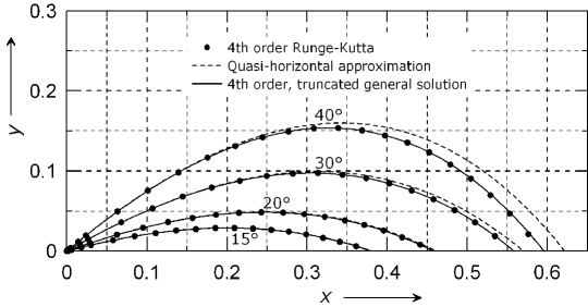
Figure 1: Trajectories for the motion of a particle under quadratic drag in a stationary medium. The units are chosen such that $\alpha=g=1$. The initial conditions are $v_{0}=1$ and (a) $\theta_{0}=15^{\circ}$, (b) $\theta_{0}=20^{\circ}$, (c) $\theta_{0}=30^{\circ}$ and (d) $\theta_{0}=40^{\circ}$. The 4th order Runge-Kutta solution of the initial value problem (14)–(17) is compared with the quasi-horizontal approximation (57) and the fourth-order solution obtained from the general solution (34)–(36).

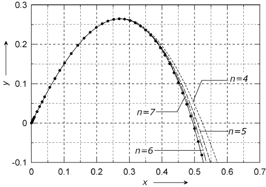
Figure 2: Trajectory of an object released at a velocity $v_{0}=1$ and an initial angle of $\theta_{0}=60^{\circ}$ in units such that $\alpha=g=1$. The numerical solution of Eqs. (14)–(17) by a 4th order Runge-Kutta method (•) is compared with the solution obtained from (35)–(36) upon truncation of $\Phi$ after the term of order $n=4,5,6,7$.

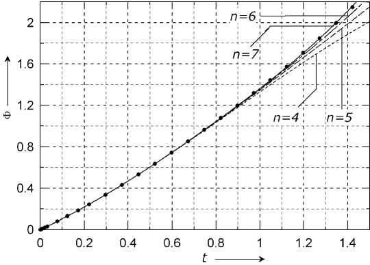
Figure 3: The resolvent variable $\Phi$ of an object released at $v_{0}=1$ and initial angle $\theta_{0}=60^{\circ}$ as a function of time. The numerical solution of (14)–(17) by a 4th order Runge-Kutta method (•) is compared with the solution obtained from (35)–(36) upon truncation of $\Phi$ after the term of order $n=4,5,6,7$.

4 Generalizations

In this section, two possible generalizations of the basic problem are discussed. First, more general drag laws are considered. Second, the requirement of constant fluid velocity is relaxed in order to include fluid velocity profiles which depend on the vertical coordinate.

4.1 Generalized Drag Laws

Here, the drag force is assumed to be of the form

$${\bf F}_{\rm d}=-m_{\rm p}\left(\alpha\|{\bf v}-{\bf V}\|^{2k}+\beta\right)\left({\bf v}-{\bf V}\right)\,,$$ (62)

where $\alpha,\beta$ and $k$ denote real non-negative constants. The reason this form of drag presents such an interesting object of study is two-fold. First, from a mathematical point of view, this law is a formal generalization of several simpler laws. Observe that setting $\alpha=0$ reduces (62) to the well-known linear Stokesian drag. For $\beta=0$, one recovers the general power law, and further setting $k=1/2$ yields Newtonian drag as used in (11). Finally, arbitrary $\alpha,\beta$ and $k=1/2$ corresponds to the generalization of the quadratic drag law proposed by Newton Newton (1687). From a physical perspective, the form of (62) comprises as a special case an often used correlation for the drag force of a sphere proposed by Schiller and Naumann Schiller and Naumann (1933). In Clift et al. (1978) it is reported that the Schiller-Naumann correlation is accurate to within $5\%$ for Reynolds numbers between $0.2$ to $10^{3}$. This drag law hence bridges the grey area between the Stokesian and the Newtonian regime.

4.1.1 Mathematical formulation

Inserting (62) into the general force balance (1) yields

$$\frac{{\rm d}{\bf v}}{{\rm d}t}=-\left(\alpha\|{\bf v}-{\bf V}\|^{2k}+\beta\right)\left({\bf v}-{\bf V}\right)+{\bf g}\;.$$ (63)

Rewriting the above in terms of the relative velocity ${\bf u}={\bf v}-{\bf V}$ and noting that ${\bf V}={\rm const.}$ yields

$$\frac{{\rm d}{\bf u}}{{\rm d}t}=-\left(\alpha\|{\bf u}\|^{2k}+\beta\right){\bf u}+{\bf g}\;.$$ (64)

In a Cartesian coordinate system identical to the one used in the previous sections, this equation may be written in components as

$$\frac{{\rm d}u_{x}}{{\rm d}t}+\left[\alpha\left(u_{x}^{2}+u_{y}^{2}\right)^{k}+\beta\right]u_{x} =0$$ (65)

$$\frac{{\rm d}u_{y}}{{\rm d}t}+\left[\alpha\left(u_{x}^{2}+u_{y}^{2}\right)^{k}+\beta\right]u_{y} =-g$$ (66)

The initial conditions are ${\bf u}(0)=\left(u_{x,0},u_{y,0}\right)$.

4.1.2 Solution

Let us begin by recasting the equations of motion into the form considered in section 2, setting $P=\alpha(u_{x}^{2}+u_{y}^{2})^{k}+\beta$ and ${\bf Q}=\left(0,-g\right)$. Observe that, as in the previous problem, $\nabla_{{\bf u}}{\bf Q}$ is still a null matrix and therefore trivially of strict lower triangular form. Therefore, this problem is of the class of equations considered in section 2 and the reduction principle may be used in order to define the appropriate resolvent variable and derive the resolvent equation:

$$\phi \equiv\exp\left\{\int_{0}^{t}\!\displaystyle\left[\alpha\left(u_{x}^{2}+u_{y}^{2}\right)^{k}+\beta\right]{\rm d}\tau\right\}$$ (67)

$$u_{x} =\frac{u_{x,0}}{\phi}$$ (68)

$$u_{y} =\frac{1}{\phi}\left(u_{y,0}-g\displaystyle\int_{0}^{t}\!\phi\,{\rm d}\tau\right)$$ (69)

$$\frac{{\rm d}\phi}{{\rm d}t} =\alpha\!\left[u_{x,0}^{2}+\left(u_{y,0}-g\int_{0}^{t}\!\phi\,{\rm d}\tau\right)^{2}\right]^{k}\phi^{1-2k}+\beta\phi$$ (70)

Introducing $\Phi$ according to (28) yields an ordinary differential equation of second order:

$$\frac{{\rm d}^{2}\Phi}{{\rm d}t^{2}}=\alpha\left[u_{x,0}^{2}+\left(u_{y,0}-g\Phi\right)^{2}\right]^{k}\left(\frac{{\rm d}\Phi}{{\rm d}t}\right)^{1-2k}+\beta\frac{{\rm d}\Phi}{{\rm d}t}\;.$$ (71)

The initial conditions remain the same as in the previous problem. A power series ansatz is now used, setting

$$\Phi=b_{0}+b_{1}t+b_{2}t^{2}+b_{3}t^{3}+\cdots$$ (72)

The initial conditions require that $b_{0}=0$ and $b_{1}=1$. All further coefficients then follow from Taylor’s theorem and may be computed recursively using

$$b_{n+2}=\frac{1}{\left(n+2\right)!}\left.\frac{{\rm d}^{n}}{{\rm d}t^{n}}\left\{\alpha\left[u_{x,0}^{2}+\left(u_{y,0}-g\Phi\right)^{2}\right]^{k}\left(\frac{{\rm d}\Phi}{{\rm d}t}\right)^{1-2k}+\beta\frac{{\rm d}\Phi}{{\rm d}t}\right\}\right|_{t=0}.$$ (73)

The first few terms of the solution hence read

$$b_{0} =0$$

$$b_{1} =1$$

$$b_{2} =\frac{\alpha u_{0}^{2k}+\beta}{2}$$

$$b_{3} =\frac{\left(1-2k\right)\alpha^{2}u_{0}^{4k}-2k\,\alpha gu_{0}^{2k-1}\sin\theta+2\left(1-k\right)\alpha\beta u_{0}^{2k}+\beta^{2}}{2\cdot 3}$$

$$\cdots \quad\,\cdots\quad\cdots\quad\cdots\quad\cdots\quad\cdots\quad\cdots\quad\cdots\quad\cdots\quad\cdots\quad\cdots\quad\cdots$$

Remark

The general nature of the coefficients is a bit more transparent if one chooses units such that $u_{0}=g=1$. Then the coefficients are bivariate polynomials in $\alpha$ and $\beta$. Each coefficient comprises terms of three different kinds. First, there are terms which depend only on $\alpha$ and thus represent the effect of the general power drag law, which is associated with high Reynolds numbers. Secondly, there are terms which represent the effect of Stokes drag, i.e. low Reynolds numbers. Other than these pure terms, there are mixed terms which are responsible for the transition between these two regimes. Although the underlying drag law is, formally, a linear superposition of a general power law and a linear law, the solution itself is not a sum of the solutions corresponding to the respective drag laws. As such, the existence of the mixed terms illustrates the nonlinearity of the problem. Nonetheless, this behaviour only becomes apparent from the third-order term onwards.

It is readily checked that upon setting $\beta=0$ and $k=1/2$, one obtains the same expansion as established in section 3 above. On the other hand, for $\alpha=0$, one obtains $\Phi=t+\beta t^{2}/2!+\beta^{2}t^{3}/3!+\cdots=\left({\rm e}^{\beta t}-1\right)/\beta$, whence $u_{x}=u_{x,0}{\rm e}^{-\beta t}$ and $u_{y}=\left(u_{y,0}+g/\beta\right){\rm e}^{-\beta t}-g/\beta$, which is the well-known closed-form solution for Stokes drag (cf. Synge and Griffith Synge and Griffith (1949), p. 159). This serves as a consistency check.

4.2 Accounting for a Velocity Profile

As a final step of generalization, the effect of velocity profiles on projectile motion is considered. After deriving the mathematical formulation, i.e. the equations of motion, the solution is obtained using the result of section 2. Finally, some properties of the solution are pointed out.

4.2.1 Equations of Motion

The equations of motion for projectile motion subject to quadratic drag in a fluid of velocity ${\bf V}$ are given by

$$\frac{{\rm d}{\bf v}}{{\rm d}t}=-\alpha\|{\bf v}-{\bf V}\|\left({\bf v}-{\bf V}\right)+{\bf g}\;.$$ (74)

The usual Cartesian coordinate system is chosen. Unlike in the previous problems, however, the fluid velocity ${\bf V}$ is now allowed to vary with height. We assume a unidirectional horizontal flow along the $x$-axis with the velocity depending only on the vertical coordinate $y$, i.e.

$${\bf V}=\left(V_{x}(y),0\right)\;,$$ (75)

so that $V_{x}$ is a sufficiently well-behaved function of $y$, subject to the condition $V_{x}(y=0)=0$. Physically, this represents a flow in the $x$-direction over a horizontal wall placed at $y=0$ with the fluid obeying the no-slip condition of a viscous fluid at a solid wall. Here, we restrict ourselves to the case where the velocity of the fluid varies linearly with height, setting $V_{x}=\gamma y.$ Such a law is valid for flows (both laminar and turbulent) close to a smooth wall. In principle, a body moving in a viscous shear flow experiences a torque proportional to its size due to the velocity gradient. In the present context, the extension of the body is assumed to be negligible compared to the velocity gradient, so that this effect can safely be disregarded. The differential equations describing the motion may then be written in coordinate form as

$$\frac{{\rm d}v_{x}}{{\rm d}t}+\alpha\left(v_{x}-\gamma y\right)\sqrt{\left(v_{x}-\gamma y\right)^{2}+v_{y}^{2}} =0$$ (76)

$$\frac{{\rm d}v_{y}}{{\rm d}t}+\alpha v_{y}\sqrt{\left(v_{x}-\gamma y\right)^{2}+v_{y}^{2}} =-g$$ (77)

The initial conditions are, as usual, $v_{x}(0)=v_{x,0}\mbox{ }\textrm{and}\mbox{ }v_{y}(0)=v_{y,0}$. In addition, it is assumed that the particle is released into the flow at $x(0)=0$ and $y(0)=y_{0}\geqslant 0$. Recalling that $v_{y}={\rm d}y/{\rm d}t$, one recognizes that due to the occurence of the vertical position $y$ the equations of motion actually constitute, in their present form, a second-order system of coupled differential equations (the second equation involving ${\rm d}v_{y}/{\rm d}t={\rm d}^{2}y/{\rm d}t^{2}$). The problem can, of course, be reformulated as a larger system of first order (including $y$ governed by ${\rm d}y/{\rm d}t=v_{y}$ as the third component). Doing so, however, violates the structure exploited in the reduction principle (7)–(8) introduced before in section 2. This inconvenience can be resolved if the problem is reformulated in terms of the relative velocity ${\bf u}={\bf v}-{\bf V}=\left(v_{x}-\gamma y,v_{y}\right)\equiv\left(u_{x},u_{y}\right)$ yielding

$$\frac{{\rm d}u_{x}}{{\rm d}t}+\alpha u_{x}\sqrt{u_{x}^{2}+u_{y}^{2}} =-\gamma u_{y}$$ (78)

$$\frac{{\rm d}u_{y}}{{\rm d}t}+\alpha u_{y}\sqrt{u_{x}^{2}+u_{y}^{2}} =-g$$ (79)

subject to the initial conditions $u_{x}(0)=u_{x,0}$ and $u_{y}(0)=u_{y,0}$.

4.2.2 Solution

In order to recast the system into the form considered in (2), the formulation of $P$ may be adopted without change from (23), since the same form of drag applies here as well. On the other hand, as an effect of the fluid velocity profile, the inhomogenous term now reads ${\bf Q}=\left(-\gamma v_{y},-g\right)$. The gradient of ${\bf Q}$ hence is

$$\nabla_{\!{\bf u}}{\bf Q}=\left(\begin{array}[]{@{}cc@{}}0&-\gamma\\ 0&{\color[rgb]{1,1,1}-}0\end{array}\right)\;,$$ (80)

i.e. no longer zero. Therefore, the traditional methods as in Bernoulli (1719) or Parker (1977) are inadequate. However, the problem is still within the scope of the reduction principle from section 2, because $\nabla_{\!{\bf u}}{\bf Q}$ is, up to numeration of indices, a strictly lower triangular matrix. The procedure then yields

$$\phi \equiv\exp\left(\alpha\displaystyle\int_{0}^{t}\!\sqrt{u_{x}^{2}+u_{y}^{2}}\,{\rm d}\tau\right)$$ (81)

$$u_{y} =\frac{1}{\phi}\left(u_{y,0}-g\displaystyle\int_{0}^{t}\!\phi\,{\rm d}\tau\right)$$ (82)

$$u_{x} =\frac{1}{\phi}\left(u_{x,0}-\gamma\displaystyle\int_{0}^{t}\!u_{y}(\phi)\,\phi\,{\rm d}\tau\right)$$ (83)

$$=\frac{1}{\phi}\left[u_{x,0}-\gamma\displaystyle\int_{0}^{t}\!\left(u_{y,0}-g\displaystyle\int_{0}^{\tau}\!\phi\,{\rm d}s\right){\rm d}\tau\right]$$ (84)

This may be further simplified by setting

$$\Psi\equiv\int\!\!\!\!\int\phi\,{\rm d}t\,{\rm d}t\;.$$ (85)

The first initial condition is imposed by the definition of $\phi={\rm d}^{2}\Psi/{\rm d}t^{2}$, namely

$$\frac{{\rm d}^{2}\Psi(0)}{{\rm d}t^{2}}=1\;.$$ (86)

Two other initial values are still necessary in order to determine $\Psi$ uniquely. This may be accomplished, e.g., by fixing the choice of integration constants in (85). The need to satisfy the physical initial conditions $u_{x}(0)=u_{x,0}$ and $u_{y}(0)=u_{y,0}$ suggests the choice

$$\Psi(0) =\frac{u_{x,0}}{g\gamma}$$ (87)

$$\frac{{\rm d}\Psi(0)}{{\rm d}t} =\frac{-u_{y,0}}{g}$$ (88)

Now, the solutions may be rewritten in terms of the auxiliary function $\Psi$ as

$$u_{x} =\,\gamma g\frac{\Psi}{{\rm d}^{2}\Psi/{\rm d}t^{2}}$$ (89)

$$u_{y} =-g\frac{{\rm d}\Psi/{\rm d}t}{{\rm d}^{2}\Psi/{\rm d}t^{2}}$$ (90)

Inserting this into (79), yields

$$\frac{{\rm d}^{3}\Psi}{{\rm d}t^{3}}=\alpha g\sqrt{\left(\gamma\Psi\right)^{2}+\left({\rm d}\Psi/{\rm d}t\right)^{2}}\;.$$ (91)

This is the new auxiliary equation to which the original coupled system has been reduced. One can now develop $\Psi$ in a power series $\Psi=c_{0}+c_{1}t+c_{2}t^{2}+c_{3}t^{3}+\cdots$ with

$$c_{n}=\frac{1}{n!}\frac{{\rm d}^{n}\Psi}{{\rm d}t^{n}}$$ (92)

according to Taylor’s theorem. The first three coefficients are given by the initial conditions. Differentiation of (91) $n$ times yields the recursive formula

$$c_{n+3}=\frac{\alpha g}{(n+3)!}\left.\frac{{\rm d}^{n}}{{\rm d}t^{n}}\sqrt{\left(\gamma\Psi\right)^{2}+\left({\rm d}\Psi/{\rm d}t\right)^{2}}\right|_{t=0},$$ (93)

which can be used to evaluate all the coefficients of the series solution, the first few terms reading

$$c_{0} =\frac{u_{0}\cos\theta_{0}}{g\gamma}$$

$$c_{1} =-\,\frac{u_{0}\sin\theta_{0}}{g}$$

$$c_{2} =1/2$$

$$c_{3} =\frac{\alpha u_{0}}{2\cdot 3}$$

$$c_{4} =-\,\frac{\alpha\left[g\sin\theta_{0}+\frac{1}{2}\gamma u_{0}\sin(2\theta_{0})\right]}{2\cdot 3\cdot 4}$$

$$\cdots \quad\,\cdots\quad\cdots\quad\cdots\quad\cdots\quad\cdots\quad\cdots$$

The solution then is

$$u_{x} =\frac{u_{x,0}}{1+\alpha u_{0}t+\cdots}-\gamma t\times\frac{u_{0}\sin\theta_{0}-\frac{1}{1\cdot 2}gt-\frac{1}{1\cdot 2\cdot 3}\alpha u_{0}gt^{2}+\cdots}{1+\alpha u_{0}t+\cdots}$$

$$u_{y} =\frac{u_{y,0}}{1+\alpha u_{0}t+\cdots}-gt\times\frac{1+\frac{1}{1\cdot 2}\alpha u_{0}t+\cdots}{1+\alpha u_{0}t+\cdots}$$

Using the transformation equations given earlier, one can deduce $v_{x},v_{y},x$ and $y$ from the above.

4.2.3 Properties

Comment on the auxiliary variable

Here, in section 4.2, the abstractly defined resolvent variable $\Psi$ no longer has the usual connotation of being (up to linear transformations) the slope of the trajectory of the projectile. This also explains why the usual approach (cf. Parker (1977)) of assuming a resolvent variable linearly related to $u_{y}/u_{x}$ is not fruitful in this case. It may be of interest to note that

$$\frac{u_{y}}{u_{x}}=-\frac{1}{\gamma\,\Psi}\frac{{\rm d}\Psi}{{\rm d}t}\;,$$ (94)

which is, up to constant factors, the logarithmic derivative of $\Psi$. From a similar point of view, the hodograph technique also appears to be problematic because expressing $\Psi$ in terms of $\tan\theta=u_{y}/u_{x}$ and inserting the resultant expression into (91) would yield an integro-differential equation involving non-trivial kernels.

Particular Solutions

Although the complete solution could not be expressed in closed form, surprisingly, there are several distinct non-trivial particular solutions that may be expressed in terms of elementary functions. To this end, assume an exponential ansatz of the form $\Psi=C\exp\left(\lambda t\right)$, where $C$ is an arbitrary constant and $\lambda\in\mathbb{C}$. Inserting this into (91) yields the characteristic equation

$$\lambda^{3}=\alpha g\sqrt{\gamma^{2}+\lambda^{2}}\;.$$ (95)

for $\lambda$. Upon squaring this equation, one obtains a bi-cubic equation with solutions $\lambda=\pm\lambda_{i}$ for $i\in\left\{1,2,3\right\}$, whereby the values $\mu_{i}=\lambda_{i}^{2}$ satisfy the cubic equation

$$\mu^{3}=\alpha^{2}g^{2}\left(\gamma^{2}+\mu\right)\;.$$ (96)

Since the principle value of the square root in (95) must be taken, this rules out one of the possible signs of $\lambda=\pm\lambda_{i}$, so that (95) indeed has three roots in $\mathbb{C}$ corresponding to three separate solutions for the set of initial conditions $\Psi(0)=C,{\rm d}\Psi(0)/{\rm d}t=\lambda C$, ${\rm d}^{2}\Psi(0)/{\rm d}t^{2}=\lambda^{2}C$. Since there is only one free parameter contained in the solution, a general set of initial conditions cannot be fulfilled, neither can the general solution be obtained by linear superposition owing to the nonlinearity of the problem. It would appear, nevertheless, that the properties of the particular solutions reflect the behaviour of the general solution, so that knowledge of the former would be instructive in comprehending the latter. This may be visualized by means of phase plots in the $\left(\Psi,{\rm d}\Psi/{\rm d}t\right)$ plane. In figure 4, a family of phase trajectories is displayed for $\gamma=1$ and various initial conditions, with $\alpha=g=1$ achieved by an appropriate choice of units. The qualitative shape may indeed be derived from the nature of the particular solutions found before. The solutions of (95) are such that one is positive real and two of them are complex conjugates with negative real part. The complex conjugate solutions are associated with exponentially damped sinusoidals, translating into a spiralling ellipse in the phase plane. Their influence, however, decays with time due to the damping. The real root, representing a growing exponential function, quickly begins to dominate the solution, so that the long-term behaviour of the solution in figure 4 is a straight line. The slope is given by the real solution of $\lambda^{3}=\sqrt{\lambda^{2}+1}$, i.e.

$$\lambda=\frac{1}{\sqrt{3}}\sqrt{\sqrt[3]{\frac{27-3\sqrt{69}}{2}}+\sqrt[3]{\frac{27+3\sqrt{69}}{2}}}\approx 1.15096$$

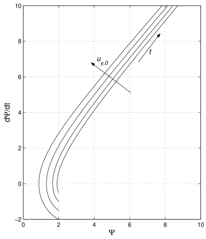
Figure 4: Family of phase trajectories for $\Psi$ in normalized units such that $\alpha=g=1$ and fixed $\gamma=1$. The initial conditions are: fixed $u_{x,0}=1$ and varying $u_{y,0}=0.5,1,1.5,\mbox{ }\textrm{and}\mbox{ }2.$

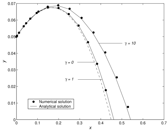
Figure 5: Situation of a particle released at $y_{0}=0.05$ in units such that $\alpha=g=1$ and with initial conditions $v_{x,0}=1,v_{y,0}=1/5$. Displayed are the trajectories for different values of the slope of the fluid velocity profile, $\gamma$. The solution obtained from truncating $\Psi$ after the fifth-order term (solid line) is compared with the numerical solution by a Runge-Kutta method. For reference, the Runge-Kutta solution without velocity profile ($\gamma=0$) is also depicted (dotted line).

5 Conclusions and Outlook

In this paper, the motion of a body in a resistant medium and a constant gravitational field was investigated. The nonlinear nature of the drag force leads to a coupled nonlinear system of ordinary differential equations, thus demanding a more involved approach in the analytical treatment. To this end, a useful technique for reducing a particular class of coupled systems of ODEs was proposed in order to facilitate the solution of such problems using analytical means.

This technique was applied to projectile motion under quadratic drag, yielding an equation of motion for a single auxiliary variable. On this basis, an exact explicit solution to the problem using elementary operations on analytic expressions was proposed. Relations to limiting cases from earlier studies were then shown. Although an exact radius of convergence could not be provided so far, the good behaviour of the solution was demonstrated by considering partial sums with different truncations. In particular, the solution was also validated numerically by comparing it with direct solutions of the original system of equations using a Runge-Kutta method. Furthermore, it was demonstrated that, when expressed in terms of appropriate variables, the constant of motion for this problem known in a different form from the literature can be interpreted as the conserved Hamiltonian of the system. Within this framework, it was further pointed out that the resolvent variable provided by the reduction principle together with its time derivative constitute the canonical or Darboux coordinates of the motion.

The reduction technique was carried over to handle a more general drag law containing quadratic and general power drag laws. A special case of this law is the Schiller-Naumann correlation valid for the transition regime between Stokesian and Newtonian drag. An exact explicit solution in the form of a ratio of time-dependent power series was presented for this case as well.

Lastly, the reduction principle was also used in order to deal with another nontrivial generalization of the basic problem, the motion of an object with quadratic drag in shear flow with a linear velocity profile. This was motivated by the fact that no study investigating projectile motion under the effect of a fluid velocity profile and nonlinear drag could be found in the literature. Again, a solution in the form of a ratio of power series was presented. Furthermore, closed-form nontrivial particular solutions for the resolvent variable were identified and the close relation between their properties and the nature of the general solution was discussed. These could be the basis of new studies, either from the perspective of the construction of a general solution from the particular solutions (nonlinear superposition) or from the point of view of semi-analytical approximations, e.g., using the method proposed by Churchill and Usagi Churchill and Usagi (1972).

While in practical applications a numerical solution of the class of systems of ODEs considered here may be more efficient in computing a solution for given initial conditions, the present results are important as they provide a means of investigating the mathematical properties of the system and, ultimately, gaining access to more physical insight, even in more general cases as demonstrated.

Several extensions of the present work are now possible: The proposed reduction technique may be applied to other ODE systems representing other phenomena, even possibly outside physics. An extension of the method to other possibly more general classes of differential equations may also be of interest.

Second, it seems appealing to generalize the shape of the background velocity profile of the fluid to some classes of nonlinear functions. Finally, the considered problem can be enhanced by considering other forces as well, of which the Magnus force presumably is the most significant, requiring an additional equation for the angular momentum of the particle.

References

- Arnol’d (1992) Arnol’d, V.I.: Ordinary Differential Equations. Springer Textbook Series, Springer Science & Business Media, New York (1992), title of the original Russian: Obyknovennye differentsial’nye uravneniya, 3rd edition, Publisher Nauka, Moscow 1984; translated by Cooke, R.
- Benacka (2010) Benacka, J.: Classroom notes: Solution to projectile motion with quadratic drag and graphing the trajectory in spreadsheets. Int. J. Math. Educ. Sci. Technol. 41(3), 373–378 (2010)
- Benacka (2011) Benacka, J.: On high-altitude projectile motion. Can. J. Phys. 89(10), 1003–1008 (2011)
- Bernoulli (1719) Bernoulli, J.: Responsio ad nonneminis provocationem, ejusque solutio quaestionis ipsi ab eodem propositae, de invenienda linea curva quam describit projectile in medio resistente. Acta Eruditorum Maji, 216–226 (1719)
- de Borda (1772) de Borda, J.C.: Sur la courbe décrite par les boulets & les bombes, en égard á la résistance de l’air. In: Histoire de l’Académie Royale des Sciences / Année M. DCCLXIX / Avec les Mémoires de Mathématique & de Physique de la même Année, Tirés des Registres de cette Académie, pp. 116–121. L’Imprimerie Royale, Paris (1772)
- Churchill and Usagi (1972) Churchill, S.W., Usagi, R.: A general expression for the correlation of rates of transfer and other phenomena. AIChE 18, 1121–1128 (1972)
- Clift et al. (1978) Clift, R., Grace, J.R., Weber, M.E.: Bubbles, Drops and Particles. Academic, New York (1978)
- Didion (1860) Didion, I.: Traité de balistique. Mallet-Bachelier, Paris, 2nd edn. (1860)
- Dominici (2003) Dominici, D.: Nested derivatives: a simple method for computing series expansions of inverse functions. Int. J. Math. Math. Sci. 2003, 3699–3715 (2003)
- Euler (1745) Euler, L.: Neue Grundsätze der Artillerie enthaltend die Bestimmung der Gewalt des Pulvers nebst einer Untersuchung über den Unterscheid des Wiederstands der Luft in schnellen und langsamen Bewegungen, aus dem Englischen des Hrn. Benjamin Robins übersezt und mit den nöthigen Erläuterungen und vielen Anmerkungen versehen von Leonhard Euler. A. Haude, Berlin (1745)
- Hackborn (2006) Hackborn, W.W.: The science of ballistics: Mathematics serving the dark side. Proc. Can. Soc. Hist. Phil. Math. 19, 109–119 (2006)
- Hardy (1940) Hardy, G.H.: A Mathematician’s Apology. Cambridge University Press, Cambridge (1940), reprinted in 1992
- Hayen (2003) Hayen, J.C.: Projectile motion in a resistant medium. Part I: exact solution and properties. Int. J. Nonlin. Mech. 38(3), 357–369 (2003)
- Lagrange (1809) Lagrange, J.L.: Mémoire sur la théorie générale de la variation des constantes arbitraires dans tous les problèmes de la méchanique. Mémoires de l’Institute national, classe des Sciences mathématiques et physiques 9, 257–302 (1809), reprinted in Œuvres, VI, pp. 771–804
- Lamb (1923) Lamb, H.: Dynamics. Cambridge University Press, London, 2nd edn. (1923)
- Lambert (1767) Lambert, J.H.: Mémoire sur la résistance des fluides avec la solution du problème ballistique. In: Histoire de l’Académie royale des sciences et belles-lettres á Berlin / Année M. DCCLXV, pp. 102–188. Haude et Spener, Berlin (1767)
- Le Gendre (1782) Le Gendre, A.M.: Dissertation sur la question de balistique proposée par l’Académie royale des sciences et belles-lettres de Prusse pour le prix de 1782. G. J. Decker, Berlin (1782)
- Liao (2004) Liao, S.J.: Beyond Perturbation: Introduction to the Homotopy Analysis Method. Chapman & Hall, London (2004)
- Nalpanis et al. (1993) Nalpanis, P., Hunt, J.C.R., Barret, C.F.: Saltating particles over flat beds. Journal of Fluid Mechanics 251, 661–685 (1993)
- Newton (1687) Newton, I.: Philosophiæ Naturalis Principia Mathematica. S. Pepys, London, 1st edn. (1687)
- Parker (1977) Parker, G.W.: Projectile motion with air resistance quadratic in the speed. Am. J. Phys. 45(7), 606–610 (1977)
- Schiller and Naumann (1933) Schiller, L., Naumann, A.: A drag coefficient correlation. VDI Zeitschrift 77, 318–320 (1933)
- Synge and Griffith (1949) Synge, J.L., Griffith, B.A.: Principles of Mechanics. McGraw-Hill Book Company, Toronto, 2nd edn. (1949)
- Tsuboi (1996) Tsuboi, K.: On the optimum angle of takeoff in long jump. Trans. Jap. Soc. Ind. Appl. Math 6, 393 (1996)
- Walter (2000) Walter, W.: Gewöhnliche Differentialgleichungen / Eine Einführung. Springer-Verlag, Heidelberg, 7th edn. (2000)
- Weinacht et al. (2005) Weinacht, P., Cooper, G.R., Newill, J.F.: Analytical prediction of trajectories for high-velocity direct-fire munitions. Tech. Rep. ARL-TR-3567, U.S. Army Research Laboratory (2005)
- Yabushita et al. (2007) Yabushita, K., Yamashita, M., Tsuboi, K.: An analytic solution of projectile motion with the quadratic resistance law using the homotopy analysis method. J. Phys. A-Math. Theor. 40, 8403–8416 (2007)