Breaking $so(4)$ symmetry without degeneracy lift

Abstract

We argue that in the quantum motion of a scalar particle of mass $m$ on $S^{3}_{R}$, perturbed by the trigonometric Scarf potential (Scarf I) with one internal quantized dimensionless parameter, $\ell$, the 3D orbital angular momentum, and another, an external scale introducing continuous parameter, $B$, a loss of the geometric hyper-spherical $so(4)$ symmetry of the free motion can occur that leaves intact the unperturbed ${\mathcal{N}}^{2}$-fold degeneracy patterns, with ${\mathcal{N}}=(\ell+n+1)$ and $n$ denoting the nodes of the wave function. Our point is that although the number of degenerate states for any ${\mathcal{N}}$ matches dimensionality of an irreducible $so(4)$ representation space, the corresponding set of wave functions do not transform irreducibly under any $so(4)$. Indeed, in expanding the Scarf I wave functions in the basis of properly identified $so(4)$ representation functions, we find power series in the perturbation parameter, $B$, where 4D angular momenta $K\in[\ell,{\mathcal{N}}-1]$ contribute up to the order $\left(\frac{2mR^{2}B}{\hbar^{2}}\right)^{{\mathcal{N}}-1-K}$. In this fashion, we work out an explicit example on a symmetry breakdown by external scales that retains the degeneracy. The scheme extends to $so(d+2)$ for any $d$.

1 Introduction

The theory of Lie algebras provides, in terms of its invariants, a power tool for the description of observed constants of motion both in free and interacting systems and enables in this manner uncovering of universal physical laws. In spectral problems, symmetry as a rule is signaled by energy values degenerate with respect to certain sets of quantum numbers, an indication that a Lie algebra might exist whose irreducible representations have dimensionalities that match the number of states in the levels. In this fashion, a relationship between symmetry and degeneracy can be established. Any ${N}$-fold degenerate system is $gl({N},R)$ symmetric in so far as by virtue of Sturm-Liouvill’s theory of differential equations, any linear superposition of solutions characterized by a common eigenvalue is again a solution to the same eigenvalue. The case of our interest here is the one in which the degeneracy patterns can be mapped on the irreducible representations of a Lie algebra distinct from $gl({N},R)$. Popular examples are the spectra of the Harmonic-Oscillator–, and the Coulomb problems, whose Hamilton operators can be cast in their turn as $su(3)$, and $so(4)$ invariants, respectively. Especially in the latter case, the ${\mathcal{N}}^{2}$-fold degeneracies of the states in a level (${\mathcal{N}}$ being the principal quantum number, ${\mathcal{N}}=n+\ell+1\in[1,\infty)$, and $\ell$ and $n$ denoting the orbital angular momentum value, and the number of nodes, respectively) has been explained in terms of $so(4)$ irreducible representations of dimensionalities, ${\mathcal{N}}^{2}$. It has been realized already in the early days of quantum mechanics that a Hamiltonian with Coulombic interaction can be cast in the form of a Casimir invariant of the isometry algebra $so(4)$ of the three-dimensional (3D) sphere, $S^{3}_{R}$ with $R$ being the hyper-radius Fock . This example shows that a relationship between symmetry and degeneracy can be at the very root of spectroscopic studies, a reason for which it is important to understand as to what extent Lie-algebraic degeneracy patterns are at par with the correct transformation properties of the wave functions under the algebra in question. Our point is that degeneracy alone is not sufficient to claim a particular Lie algebraic symmetry of the Hamiltonian. On the example of the quantum motion of a scalar particle on $S^{3}_{R}$, perturbed by the trigonometric Scarf potential (Scarf I), we show that the perturbation completely retains the $so(4)$ degeneracies of the free motion without that the “perturbed” wave functions would behave as eigenfunctions of an $so(4)$ Casimir operator.

The contribution is structured as follows. In the next section we study the $so(4)$ symmetry properties of the hyper-geometric differential equation for the Gegenbauer polynomials, ${\mathcal{G}}_{n}^{\lambda}(x)$, for $\lambda=(\ell+1)$ with $\ell$ non-negative integer. First we observe that in subjecting the eigenvalue problem of the canonical $so(4)$ Casimir operator to a similarity transformation by $(1-\sin^{2}\chi)^{\frac{\lambda}{2}-\frac{1}{4}}$, the square-root of the weight function of the Gegenbauer polynomials, and setting $x=\sin\chi$, with $\chi$ standing for the second polar angle in $E_{4}$, amounts to the Gegenbauer equation, thus making the $so(4)$ symmetry of the latter manifest. As long as free quantum motion on $S^{3}_{R}$ can be cast as the eigenvalue problem of the Casimir operator of the transformed $so(4)$, whose wave functions are the Gegenbauer polynomials, $so(4)$ has been proved to be the relevant symmetry both of the spectrum and the wave functions. This contrasts the case of the Jacobi polynomials, $P_{n}^{\alpha\beta}(x)$, considered in section III for the following parameter values, $\alpha_{\ell}=\ell+\frac{1}{2}-b$, and $\beta_{\ell}=\ell+\frac{1}{2}+b$, which present themselves as linear combinations of Gegenbauer polynomials of equal $\lambda=(\ell+1)$ parameters but different degrees, $n$, and do not behave as $so(4)$ representation functions. Nonetheless, because of the above specific choice of the parameters, the Jacobi polynomial equation can be transformed to a motion on $S^{3}_{R}$ perturbed by the trigonometric Scarf potential, whose spectrum carries by chance same $so(4)$ degeneracy patterns as the free motion, without that this symmetry is shared by the wave functions. In this manner, we explicitly work out an example of breaking $so(4)$ by a perturbation without degeneracy lift. The paper closes with brief conclusions.

2 The Gegenbauer polynomial equation as eigenvalue problem of an $so(4)$ Casimir operator

The Gegenbauer polynomial equation Abr for the special choice of the parameter, $\lambda=\ell+1$, with $\ell$ non-negative integer, is given by

$$\left(1-x^{2}\right)\frac{{\mathrm{d}}^{2}{\mathcal{G}}_{n}^{\ell+1}(x)}{{\mathrm{d}}x^{2}}-\left(2\ell+3\right)x\frac{{\mathrm{d}}{\mathcal{G}}_{n}^{\ell+1}(x)}{{\mathrm{d}}x}+n(n+2\ell+2){\mathcal{G}}_{n}^{\ell+1}(x)=0.$$ (1)

At the same time, the eigenvalue problem of the well known Casimir operator, ${\mathcal{K}}^{2}$, of the $so(4)$ isometry algebra of the three dimensional (3D) unit sphere, to be denoted by $S^{3}$, reads

$$\left[{\mathcal{K}}^{2}-K(K+2)\right]Y_{K\ell m}(\chi,\theta,\varphi)=0,\,\,{\mathcal{K}}^{2}=\frac{(-1)}{\cos^{2}\chi}\frac{\partial}{\partial\chi}\cos^{2}\chi\frac{\partial}{\partial\chi}+\frac{{\mathbf{L}}^{2}(\theta,\varphi)}{\cos^{2}\chi},$$

$$Y_{K\ell m}(\chi,\theta,\varphi)=\cos^{\ell}\chi{\mathcal{G}}_{n=K-\ell}^{\ell+1}(\sin\chi)Y_{\ell m}(\theta,\varphi),\,\,\quad K=n+\ell,$$

$${\mathbf{L}}^{2}(\theta,\varphi)Y_{\ell m}(\theta,\varphi)=\ell(\ell+1)Y_{lm}(\theta,\varphi).\,\,\qquad\qquad$$ (2)

Here, ${\mathbf{L}}(\theta,\varphi)$ is the 3D angular momentum operator, $K$, $\ell$ and $m$ are in turn the 4D-, 3D, and 2D angular momentum values, $Y_{K\ell m}(\chi,\theta,\varphi)$ are the 4D spherical harmonics, with $\chi\in\left[-\frac{\pi}{2},+\frac{\pi}{2}\right]$, and $\theta\in\left[0,\pi\right]$ standing for the two polar angles parametrizing $S^{3}$, and $\varphi\in\left[0,2\pi\right]$ denoting the ordinary azimuthal angle. In the so called quasi-radial variable Kalnin , $\chi$, the equation  (2) reduces to

$$\left[-\frac{1}{\cos^{2}\chi}\frac{\partial}{\partial\chi}\cos^{2}\chi\frac{\partial}{\partial\chi}+\frac{\ell(\ell+1)}{\cos^{2}\chi}-K(K+2)\right]\cos^{\ell}\chi{\mathcal{G}}_{K-\ell}^{\ell+1}(\sin\chi) = 0,$$ (3)

and it is straightforward to check that (3) is equivalent to

$$\left[{\widetilde{\mathcal{K}}}^{2}-(n+l)(n+l+2))\right]{\mathcal{G}}_{K-\ell}^{\ell+1}(\sin\chi) = 0,$$

$$\mbox{ with}\qquad{\widetilde{\mathcal{K}}}^{2}=\cos^{-\ell}\chi{\mathcal{K}}^{2}\cos^{\ell}\chi,$$ (4)

because of

$${\widetilde{\mathcal{K}}}^{2}=\cos^{-\ell}\chi{\mathcal{K}}^{2}\cos^{\ell}\chi = -\frac{{\mathrm{d}}^{2}}{{\mathrm{d}}\chi^{2}}+\left(2\ell+2\right)\tan\chi\frac{{\mathrm{d}}}{{\mathrm{d}}\chi}+\ell(\ell+2).$$ (5)

The $\cos^{\ell}\chi$ function relates to the square-root of the weight function, $\omega^{\lambda}(x)$, of the Gegenbauer polynomials, ${\mathcal{G}}_{n}^{\lambda}(x)$, as,

$$\omega^{\lambda}(x)=(1-x^{2})^{\lambda-\frac{1}{2}}, x=\sin\chi,\quad\lambda=(\ell+1),$$

$$\cos^{\ell}\chi = \sqrt{\frac{\omega^{\ell+1}(\sin\chi)}{\frac{{\mathrm{d}}x}{{\mathrm{d}}\chi}}}.$$ (6)

Therefore, upon changing variable in (5) to $x=\sin\chi$, and back-substituting in (3), one obtains the claimed equality between the $so(4)$ Null operator,

$$\left[{\widetilde{\mathcal{K}}}^{2}-K(K+2)\right],\quad K=n+\ell,$$ (7)

and the Gegenbauer polynomial equation as,

$$\left[{\widetilde{\mathcal{K}}}^{2}-(n+l)(n+l+2)\right]{\mathcal{G}}_{K-\ell}^{\ell+1}(x) = \left(1-x^{2}\right)\frac{{\mathrm{d}}^{2}{\mathcal{G}}_{K-\ell}^{\ell+1}(x)}{{\mathrm{d}}x^{2}}-\left(2\ell+3\right)\frac{{\mathrm{d}}{\mathcal{G}}^{\ell+1}_{K-\ell}(x)}{{\mathrm{d}}x}$$ (8)

$$+ n(n+2\ell+2){\mathcal{G}}_{{K-\ell}}^{\ell+1}(x)=0.$$

The latter equation means that the Gegenbauer polynomials, occasionally termed to as ultra-spherical polynomials, are representation functions to an $so(4)$ algebra obtained from the canonical one according to (6) through a similarity transformation by the square-root of their weight function and upon accounting for a change of variable. An interesting connection between the latter equation and the 1D Schrödinger equation with the $\sec^{2}\chi$ potential can be established upon substituting,

$$\cos^{\ell}\chi{\mathcal{G}}_{K-\ell}^{\ell+1}(\sin\chi)=\frac{{\mathcal{U}}_{n}^{\ell}(\chi)}{\cos\chi},\quad n=K-\ell.$$ (9)

In so doing, one finds that ${\mathcal{U}}_{n}^{\ell}(\chi)$ satisfies the 1D Schrödinger equation with the $\sec^{2}\chi$ potential according to,

$$\left[-\frac{{\mathrm{d}}^{2}}{{\mathrm{d}}\chi^{2}}+\frac{\ell(\ell+1)}{\cos^{2}\chi}\right]{\mathcal{U}}_{n}^{\ell}(\chi)=(K+1)^{2}{\mathcal{U}}_{n}^{\ell}(\chi),$$ (10)

whose spectrum is characterized by $(K+1)^{2}$-fold degeneracy of the levels, just as the H atom, due to $\sum_{\ell=0}^{\ell=K}(2\ell+1)=(K+1)^{2}$. Therefore, the $so(4)$ symmetry of the Gegenbauer polynomials shows up as $so(4)$ degeneracy patterns in the spectrum of the corresponding 1D Schrödinger equation with the $\sec^{2}\chi$ interaction. More general, there are several two-parameter potentials, $v(z;\alpha,\beta)$ for which the Schrödinger equation,

$$\left[-\frac{{\mathrm{d}}^{2}}{{\mathrm{d}}z^{2}}+v(z;\alpha,\beta))\right]R^{\alpha\beta}_{n}(z)=\epsilon R^{\alpha\beta}_{n}(z),$$ (11)

can be exactly solved by reducing it to a hyper-geometric differential equation by means of a point-canonical transformation of the type Levai ,

$$R_{n}^{\alpha\beta}(z)=R_{n}^{\alpha\beta}\left(z=f(x)\right):\stackrel{{\scriptstyle\mbox{\footnotesize def}}}{{=}}g^{\alpha\beta}_{n}(x)=\sqrt{\omega^{\alpha\beta}(x)}J_{n}^{\alpha\beta}(x)\frac{1}{\sqrt{\frac{{\mathrm{d}}f(x)}{{\mathrm{d}}x}}},\quad x\in[a,b],$$ (12)

where $J_{n}^{\alpha\beta}(x)$ are polynomials of degree $n$ and orthogonal with respect to their weight-function $\omega^{\alpha\beta}(x)$ according to

$$\int_{0}^{\infty}R^{\alpha\beta}_{n}(z)R^{\alpha\beta}_{n^{\prime}}(z){\mathrm{d}}z=\int_{a}^{b}g_{n}^{\alpha\beta}(x)g_{n^{\prime}}^{\alpha\beta}(x){\mathrm{d}}f(x)=\int_{a}^{b}\omega^{\alpha\beta}(x)J_{n}^{\alpha\beta}(x)J_{n^{\prime}}^{\alpha\beta}(x){\mathrm{d}}x.$$ (13)

And vice verse, any hyper-geometric differential equation can be brought back to an 1D Schrödinger equation in (11) by inverting the transformation in (12).

The above procedure establishes an interesting link between the symmetry properties of orthogonal polynomials and the degeneracies in the corresponding potential spectra. In the next subsection we shall see that a Lie algebraic degeneracy in the Schrödinger spectrum can appear by chance and without it being shared by the polynomial equation.

3 A Jacobi polynomial equation as eigenvalue problem of a “frustrated” $so(4)$ Casimir operator

The hyper-geometric differential equation solved by the Jacobi polynomial reads Abr ,

$$\left(1-x^{2}\right)\frac{{\mathrm{d}}^{2}{P}_{n}^{\alpha\beta}(x)}{{\mathrm{d}}x^{2}}+\left[(\beta-\alpha)-\left(\alpha+\beta+2\right)x\right]\frac{{\mathrm{d}}{P}_{n}^{\alpha\beta}(x)}{{\mathrm{d}}x}+n(n+\alpha+\beta+1){P}_{n}^{\alpha\beta}(x)=0,$$ (14)

and acquires a shape pretty close to (1) for the following special choice of the parameters,

$$\alpha_{\ell}=\ell-b+\frac{1}{2},\quad\beta_{\ell}=\ell+n+\frac{1}{2},$$ (15)

namely,

$${\Big{(}}{\widetilde{\mathcal{K}}^{2}}-(n+\ell)(n+\ell+2)+2b\frac{{\mathrm{d}}}{{\mathrm{d}}x}{\Big{)}}{P}_{n}^{\ell-b+\frac{1}{2},\ell+b+\frac{1}{2}}(x)$$

$$=\left(1-x^{2}\right)\frac{{\mathrm{d}}^{2}{P}_{n}^{\ell-b+\frac{1}{2},\ell+b\frac{1}{2}}(x)}{{\mathrm{d}}x^{2}}+\left[2b-\left(2\ell+3\right)x\right]\frac{{\mathrm{d}}{P}_{n}^{\ell-b+\frac{1}{2},\ell+b+\frac{1}{2}}(x)}{{\mathrm{d}}x}$$

$$+n(n+2\ell+2){P}_{n}^{\ell-b+\frac{1}{2},\ell+b+\frac{1}{2}}(x)=0.$$ (16)

The latter relation reveals the Jacobi equation as the $so(4)$ Null-operator in (7), “frustrated” by the gradient term $\left[-2b\frac{{\mathrm{d}}}{{\mathrm{d}}x}\right]$. In consequence, the Jacobi polynomials do not behave as $so(4)$ representation functions. This is best illustrated through the finite series decomposition of a Jacobi polynomial of degree $n$ in Gegenbauer polynomials of degrees running from $0$ to $n$, shown in Table I. In recalling that the degrees of the Gegenbauer polynomials under considerations express in terms of the 4D angular momentum values, $K$, as $n=(K-\ell)$, the decompositions present themselves as mixtures of $so(4)$ representation functions of different 4D angular momentum values, $K\in\left[\ell,\ell+n\right]$.

Despite the absence of $so(4)$ symmetry of the Jacobi polynomials, a curiosity occurs insofar as the associated 1D Schrödinger equation (in units of $\hbar^{2}/(2mR^{2})$),

$$\left[-\frac{{\mathrm{d}}^{2}}{{\mathrm{d}}\chi^{2}}+v_{\mbox{\footnotesize ScI}}\left(\chi;\alpha_{\ell},\beta_{\ell}\right)\right]\,R_{n}^{\ell-b+\frac{1}{2},\ell+b+\frac{1}{2}}\left(\chi\right)=\epsilon\,R_{n}^{\ell-b+\frac{1}{2},\ell+b+\frac{1}{2}}\left(\chi\right),$$ (17)

$$v_{\textup{ScI}}\left(\chi;\alpha_{\ell},\beta_{\ell}\right)=\frac{b^{2}+\ell(\ell+1)}{\cos^{2}\chi}-\frac{b(2\ell+1)\tan\chi}{\cos\chi},\,\,b=\frac{B(2mR^{2})}{\hbar^{2}},$$ (18)

$$R_{n}^{\ell-b+\frac{1}{2},\ell+b+\frac{1}{2}}\left(\chi\right)=e^{-b\tanh^{-1}\sin\chi}\cos^{\ell+1}\chi P_{n}^{\ell-b+\frac{1}{2},\ell+b+\frac{1}{2}}\left(\sin\chi\right),$$ (19)

$${\mathcal{N}}=n+\ell+1,\quad\epsilon={\mathcal{N}}^{2},\quad\epsilon=\frac{E(2mR^{2})}{\hbar^{2}},[E],[B]=\mbox{MeV},$$ (20)

reduced to the hyper-geometric differential equation along the line of the above eqs. (13)–(12) for $\chi=f(x)=\sin^{-1}x$, and

$$\omega^{\ell-b+\frac{1}{2},\ell+b+\frac{1}{2}}(x)=e^{-b\tanh^{-1}x}(1-x^{2})^{\ell+\frac{1}{2}},$$ (21)

exhibits same degeneracy patterns as the fully $so(4)$ symmetric problem in (10) and the underlying (8). In (18), the $v_{\mbox{\footnotesize ScI}}\left(\chi;\alpha_{\ell},\beta_{\ell}\right)$ potential is known under the name of the trigonometric Scarf potential, abbreviated, Scarf I (Levai and references therein). Under the substitution,

$$R_{n}^{\ell-b+\frac{1}{2},\ell+b+\frac{1}{2}}\left(\chi\right)=\frac{U_{n}^{\ell-b+\frac{1}{2},\ell+b+\frac{1}{2}}\left(\chi\right)}{\cos\chi},$$ (22)

the equation (18) is transformed to motion on $S^{3}$ perturbed by Scarf I. The expansions in Table I apply equally well to the wave functions $U_{n}^{\ell-b+\frac{1}{2},\ell+b+\frac{1}{2}}\left(\chi\right)$ which can not transform as $so(4)$ representation functions despite the $so(4)$ degeneracy patterns in the spectrum. In this fashion, we worked out an example that a Lie algebraic symmetry in a spectral problem does not necessarily imply same symmetry of the Hamiltonian. The Figure 1 is illustrative of this type of $so(4)$ breaking.

Table 1: Decompositions of some of the Jacobi polynomials $P_{n}^{\ell-b+\frac{1}{2},\ell+b+\frac{1}{2}}(\sin\chi)$ in (15) for fixed $\ell$ in $so(4)$ representation functions of 4D angular momenta $K\in\left[\ell\,,\kappa\right]$ with $\kappa=n+\ell={\mathcal{N}}-1$. The $K$ labeled Gegenbauer polynomials contribute to the order ${\mathcal{O}}\left(b^{\kappa-K}\right)$ to the expansion and give the order to which the $so(4)$ symmetry fades away, with $b$ defined in (15) and (18).

$\ell$	K	$P_{n=\kappa-{\ell}}^{(\alpha_{\ell},\beta_{\ell})}(\sin\chi)$	=	$\sum_{{K}={\ell}}^{\kappa}c_{K\kappa}(b)\,\mathcal{G}_{K-{\ell}}^{{\ell}+1}(\sin\chi)$
$\kappa$	K=$\kappa$	$P_{0}^{(\alpha_{k},\beta_{k})}(\sin\chi)$	=	$\mathcal{G}_{0}^{k+1}(\sin\chi)$
$\kappa-1$	K$\in\left[\kappa-1,\kappa\right]$	$P_{1}^{(\alpha_{k-1},\beta_{k-1})}(\sin\chi)$	=	$\frac{(2k+1)}{4k}\,\mathcal{G}_{1}^{k}(\sin\chi)-b\,\mathcal{G}_{0}^{k}(\sin\chi)$
$\kappa-2$	K $\in\left[\kappa-2,\kappa\right]$	$P_{2}^{(\alpha_{k-2},\beta_{k-2})}(\sin\chi)$	=	${1\over 8}\frac{(2k+1)}{(k-1)}\,\mathcal{G}_{2}^{k-1}(\sin\chi)-{b\over 2}\frac{k}{(k-1)}\,\mathcal{G}_{1}^{k-1}(\cot\chi)+\frac{b^{2}}{2}\,\mathcal{G}_{0}^{k-1}(\sin\chi)$
$\kappa-3$	K$\in\left[\kappa-3,\kappa\right]$	$P_{3}^{(\alpha_{k-3},\beta_{k-3})}(\sin\chi)$	=	${1\over 32}\frac{(4\kappa^{2}-1)}{(\kappa^{2}-3\kappa+2)}\,\mathcal{G}_{3}^{(k-2)}(\sin\chi)-{b\over 8}\frac{(2\kappa^{2}-\kappa)}{(\kappa^{2}-3\kappa+2)}\,\mathcal{G}_{2}^{(k-2)}(\sin\chi)+{b^{2}\over 8}\frac{(2k-1)}{(k-2)}\,\mathcal{G}_{1}^{(k-2)}(\sin\chi)$
				$-{b\over 24}\frac{(4b^{2}k-4b^{2}+2k+1)}{(k-1)}\,\mathcal{G}_{0}^{(k-2)}(\sin\chi)$

[scale=.4]degenerado3.eps

Figure 1: The breaking of the $so(4)$ symmetry of the free motion of a scalar particle on $S^{3}$ in (3)-(5) and (10), through the external scale $B=\frac{\hbar^{2}b}{2mR^{2}}$, due to a perturbation by the trigonometric Scarf potential (17)–(20). The wave function $U_{3}^{\frac{3}{2}-b,\frac{3}{2}+b}(\chi)$ in (22) (right) in comparison to its counterpart, $\cos^{\ell}\chi{\mathcal{G}}_{3}^{2}(\sin\chi)$ in (4) (left) describing the unperturbed $so(4)$ symmetric motion. These functions describe equal energies in the respective potential problems in eqs. (10) and (20).

t]

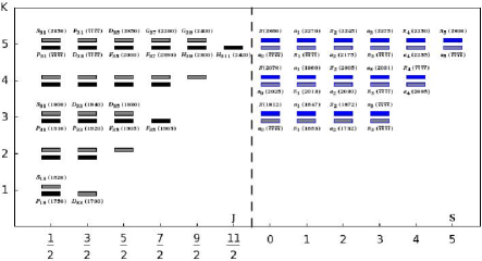
Figure 2: Hydrogen like (conformal type) degeneracy in the reported spectra of the excited $L_{3(2J)}$, i.e. $\Delta$ baryons (left) and the high-lying light flavored mesons (right) (for details on the notations and more references see Kirchbach2010 ,PART ). Full and shadowed bricks denote degenerate hadron states of opposite parities. The numbers inside of the parenthesis give the masses (in MeV) while the question marks denote “missing” states. The meson sector is close to parity doubled, a possible hint on chiral symmetry restoration from the spontaneously broken Nambu-Goldstone– to the manifest Wigner-Wyle mode. Remarkable, the pronounced supersymmetric baryon-meson degeneracy.

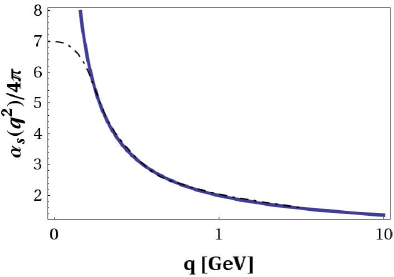
Figure 3: Schematic presentation of the walking (dashed line) of the strong coupling constant in the infrared according to Deur .

4 Conclusions

In this work we constructed an explicit example for the possibility to remove a Lie algebraic symmetry of a Hamiltonian by perturbation and without lifting the unperturbed degeneracy patterns in the spectrum. The clue of this observation is that Lie algebraic degeneracy patterns can throughout be tolerant towards external scales, such as masses, temperatures, lengths etc. Such a type of $so(4)$ symmetry lift could reconcile the experimentally detected conformal symmetry patterns in the spectra of the high-lying light flavored hadrons, both baryons and mesons, with the conformal symmetry removal through the dilaton mass. The relevance of the conformal symmetry for QCD is predicted by the AdS₅/CFT₄ duality and is compatible with spectroscopic data on the light-flavored hadron spectra (see Fig. 2) due to the walking of the strong coupling constant in the infrared towards a fixed value Deur , sketched in Fig. 3. The relevance of the hyper-spherical geometry in conformal field theories is derived from the possibility of mapping a flat space-time QFT on Einstein’s closed universe, ${\mathcal{R}}^{1}\otimes S^{3}_{R}$, whose isometry algebra is the covering of the conformal one, a result due to LuMack . The so called compactified Minkowski space time, in being of finite 3D volume, provides a natural scenario for the QCD confinement phenomenon Witten and the inverse of the $S^{3}_{R}$ radius provides a natural scale that can be interpreted as the temperature Tommy .

References

• (1)
• (2) V. A. Fock, Zur Theorie des Wasserstoffatoms, Z.Β Phys.Β 98 (1935) 145-154
• (3) M.Β  Abramovic and I.Β A.Β Stegun, Handbook of mathematical functions with formulas, graphs and tables (Dover publications, Inc., New York, 1972)
• (4) E.Β Kalnins, W.Β Miller, and G.Β S.Β Pogosyan, The Coulomb-oscillator relation on n-dimensional spheres, Physics of Atomic Nuclei 65 (2002) 1086-1094
• (5) G.Β Levai, Solvable potentials associated with su(1,1) algebras:a systematic study, J.Β Phys.Β A:Math. Gen. 27 (1994) 3809-3828
• (6) A.Β Deur, V.Β  Burker, J.Β P.Β  Chen, and W.Β Korsch, Determination of the effective strong coupling constant alpha(s, g(1)) (Q**2) from CLAS spin structure function data, Phys.Β Lett. 665 (2008) 349-351
• (7) M.Β Kirchbach and C.Β Compean, Conformal symmetry and light flavor baryon spectra, Phys.Β Rev.Β  D 82Β  (2010) 034008
• (8) M.Β LΓΌscher and G.Β Mack, Global conformal invariance in quantum field theory, Comm. Math. Phys. 41 (1975) 203-234
• (9) E. Witten, Anti de Sitter space and holography, Adv.Β Theor.Β Math.Β Phys.Β 2 (1998) 233-291
• (10) S.Β Hands, T.Β J.Β Hollowood, and J.Β C.Β  Myers, QCD with chemical potential in a small hyperspherical box, JHEP 1007 (2010) 086
• (11) J.Β Beringer et al.(Particle Data Group), Review of Particle Physics, Phys.Β Rev.Β D 86 (2012), 010001