Weak-coupling analysis of the single-site large-N gauge theory coupled to adjoint fermions

Abstract

We consider the leading-order expression at weak coupling for a single-site large-$N$ gauge theory coupled to adjoint fermions. We study the case of overlap and Wilson fermions. We extend the theory to real values of the number of fermion flavors and restrict ourselves to asymptotically free theories. Using a four-dimensional density function for the distribution of the eigenvalues of the link variables, we show that it is possible to recover the infinite-volume continuum limit for a certain range of fermion flavors if we use fermions with a bare mass of zero. Our use of the four-dimensional density function is supported by a direct analysis of the lattice action.

I Introduction

Nonabelian gauge field theories coupled to fermions in some representation of the gauge group are asymptotically free as long as the number of fermion flavors is less than a certain number. Within this allowed range of fermion flavors, the theory is expected to be confining in some range at the lower end and it is expected to be conformal at the higher end. Identification of the critical number of fermion flavors that separate the confining region from the conformal region is a non-perturbative task that has recently received considerable attention within the lattice field theory community Hasenfratz:2013uha –Appelquist:2007hu . Several issues need to be resolved before such an endeavor can make some physics conclusions. These include (a) How does one deal with a conformal theory on a lattice; (b) How does one conclude that a certain model exhibits features of near conformal features; (c) How does one compute the location of the infra-red fixed point in a lattice model. Since finite-volume effects need to be understood carefully and since one has to be close to the chiral limit to understand the above issues, the numerical simulations are inherently large scale in nature.

An attractive alternative has been proposed to study large-$N$ gauge field theories coupled to adjoint fermions on a single-site lattice. It has been argued that reduction to a single-site lattice should hold in such theories Kovtun:2007py and tested numerically using a variety of methods to see if one can reproduce the continuum infinite-volume theory by working on a single-site lattice Bedaque:2009md –Gonzalez-Arroyo:2013gpa . With the exception of Gonzalez-Arroyo:2013gpa ; GonzalezArroyo:2012st , all attempts have considered the Eguchi-Kawai reduction and numerically argued that the single-site theory is in the correct continuum phase. Asymptotic freedom is maintained in these theories if the number of Dirac flavors is less than $\frac{11}{4}$. Two-loop perturbative beta function would suggest the existence of an infra-red fixed point if the the number of fermion flavors is greater than $\frac{17}{16}$. With this in perspective, the single-site model with one massless adjoint overlap-Dirac fermion was extensively studied in Hietanen:2012ma . Numerical results suggest that the coupling runs much faster than what is predicted by continuum two-loop perturbation theory at the lattice couplings that were considered. In order to better understand the connection between single-site lattice models and infinite-volume continuum theories, we decided to revisit the problem of perturbation theory on the single-site lattice in this paper.

We will consider the weak-coupling limit and the only parameters we will consider are the number of fermion flavors which we will extend to take on all real values in the range $\left[0,\frac{11}{4}\right]$ and the fermion mass. The main aim of this paper is to use a four-dimensional density function to answer two questions:

1. What is the range of fermion flavors for which the single-site massless theory can be expected to reproduce the infinite-volume continuum theory?

2. Can we reproduce the infinite-volume continuum theory with massive fermions?

We will provide an answer to both these questions using Wilson fermions and overlap fermions. We will not consider the case of twisted reduction in this paper.

II The single-site model

The single-site partition function for a $\operatorname{SU}(N)$ gauge theory coupled to $f$ flavors of fermions in the adjoint representation is

$$Z=\int\prod_{\mu}dU_{\mu}e^{S_{g}+fS_{f}}$$ (1)

with Haar measure $dU$. The Wilson gauge action is

$$S_{g}=bN\sum_{\mu,\nu=1}^{d}\operatorname{Tr}\left[U_{\mu}U_{\nu}U_{\mu}^{\dagger}U_{\nu}^{\dagger}-1\right].$$ (2)

The fermion action is

$$S_{f}=\ln\det H_{w,o}$$ (3)

with the subscript $w$ for Wilson fermions and $o$ for overlap fermions. The Hermitian Wilson Dirac operator for massive adjoint fermions is given by

$$H_{w}(m_{w})=\begin{pmatrix}4+m_{w}-\frac{1}{2}\sum_{\mu}\left(A_{\mu}+A_{\mu}^{t}\right)&\frac{1}{2}\sum_{\mu}\sigma_{\mu}\left(A_{\mu}-A_{\mu}^{t}\right)\cr-\frac{1}{2}\sum_{\mu}\sigma^{\dagger}_{\mu}\left(A_{\mu}-A_{\mu}^{t}\right)&-4-m_{w}+\frac{1}{2}\sum_{\mu}\left(A_{\mu}+A_{\mu}^{t}\right)\cr\end{pmatrix}\,,$$ (4)

where $m_{w}$ is the bare Wilson fermion mass. The adjoint gauge fields are given by

$$A_{\mu}^{ab}=\frac{1}{2}\operatorname{Tr}\left[T^{a}U_{\mu}T^{b}U^{\dagger}_{\mu}\right],$$ (5)

where $T^{a}$, $a=1,\ldots,(N^{2}-1)$ are traceless Hermitian matrices that generate the $\operatorname{su}(N)$ Lie algebra and satisfy

$$\operatorname{Tr}T^{a}T^{b}=2\delta^{ab}\,;\ \ \ \ [T^{a},T^{b}]=\sum_{c}if^{ab}_{c}T^{c}.$$ (6)

The Hermitian massive overlap Dirac operator is defined by

$$H_{o}(m_{o})=\frac{1}{2}\left[\left(1+m_{o}\right)\gamma_{5}+\left(1-m_{o}\right)\epsilon\left[H_{w}(m_{w})\right]\right]\,,$$ (7)

where $m_{o}\in[0,1]$ is the bare overlap fermion mass and $m_{w}<0$ is the irrelevant Wilson mass parameter.

The total action depends on $d$ $\operatorname{SU}(N)$ matrices and the gauge transformation is

$$U_{\mu}\to gU_{\mu}g^{\dagger}.$$ (8)

Note that the eigenvalues of $U_{\mu}$ are gauge invariant. We cannot fix a gauge such that one of the $U_{\mu}=1$ since we are on a single-site lattice. The action has an additional $\operatorname{U}^{d}(1)$ symmetry given by

$$U_{\mu}\to e^{i\alpha_{\mu}}U_{\mu}$$ (9)

with $0\leq\alpha_{\mu}<2\pi$. Restricting $\alpha_{\mu}$ to $\frac{2\pi k_{\mu}}{N}$ with integers $0\leq k_{\mu}<N$ keeps it in $\operatorname{SU}(N)$; otherwise we have trivially extended the $\operatorname{SU}(N)$ theory to a $\operatorname{U}(N)$ theory. The four Polyakov loop operators, given by

$$P_{\mu}=\operatorname{Tr}U_{\mu}\,,$$ (10)

are gauge invariant but not invariant under (9). If the $\operatorname{U}^{d}(1)$ symmetry is not broken, then the eigenvalues of all $U_{\mu}$ are uniformly distributed on the unit circle and $P_{\mu}=0$ (the reverse statement is not necessarily true because the eigenvalues in different directions might be correlated). In the following, we set the number of Euclidean space-time dimensions $d$ to $4$.

III Leading-order perturbation theory and the density function

The symmetry given by (9) is spontaneously broken in the weak-coupling limit if we do not have adjoint fermions even when there are a finite number of flavors of fundamental fermions Bhanot:1982sh . We want to study if this symmetry is spontaneously broken in the weak-coupling limit in the presence of adjoint fermions. We set

$$U_{\mu}=V_{\mu}D_{\mu}V^{\dagger}_{\mu}\,;\ \ \ \ D_{\mu}^{jk}=e^{i\theta^{j}_{\mu}}\delta^{jk},$$ (11)

and expand around $V_{\mu}=1$ to compute observables in perturbation theory.

The expression for the partition function at leading order at weak coupling is known Hietanen:2009ex and is given by

$$Z^{0} =\int\left[\prod_{\mu}\prod_{i}d\theta^{i}_{\mu}\right]e^{S^{0}}\,; S^{0} =S_{g}^{0}+fS_{f}^{0}\,;$$ (12)

$$S_{g}^{0} =-\sum_{i\neq j}\ln\hat{p}^{ij}\,; \hat{p}^{ij} =\sum_{\mu}4\sin^{2}\frac{\theta_{\mu}^{i}-\theta_{\mu}^{j}}{2}\,.$$ (13)

The fermionic contribution is

$$S_{w,o}^{0}=2\sum_{i\neq j}\ln\gamma_{w,o}^{ij}(m_{w,o})\,,$$ (14)

where we have removed a $\theta$-independent term that arises from the zero modes for massless fermions and assumed that $\hat{p}^{ij}\neq 0$ if $i\neq j$. The non-zero modes are given by

$$\gamma_{w}^{ij}(m_{w}) =\left(m_{w}+\frac{\hat{p}^{ij}}{2}\right)^{2}+\bar{p}^{ij}\,;\qquad\qquad\bar{p}^{ij}=\sum_{\mu}\sin^{2}\left(\theta_{\mu}^{i}-\theta_{\mu}^{j}\right)\,;$$ (15)

$$\gamma_{o}^{ij}(m_{o},m_{w}) =\frac{1+m_{o}^{2}}{2}+\frac{1-m_{o}^{2}}{2}\frac{m_{w}+\frac{\hat{p}^{ij}}{2}}{\sqrt{\gamma_{w}^{ij}(m_{w})}}\,.$$ (16)

Owing to the symmetry given by (9) $S^{0}$ is invariant under $\theta_{\mu}^{i}\to\theta_{\mu}^{i}+\alpha_{\mu}$ for any choice of $\alpha_{\mu}$.

As $N\to\infty$, we assume that we can define a joint distribution, $\rho(\theta)$, in the following sense: At any finite $N$, for a fixed choice of $\theta_{\mu}^{i}$, $i=1,\ldots,N$ and $\mu=1,\ldots,4$, let

$$\rho(\theta)=\frac{1}{N}\sum_{i}\prod_{\mu}\delta(\theta_{\mu}-\theta_{\mu}^{i})\,;\qquad\qquad\int\prod_{\mu}d\theta_{\mu}\rho(\theta)=1\,,$$ (17)

where $\delta$ denotes the $2\pi$-periodized delta function normalized to $\int_{-\pi}^{\pi}d\theta\delta(\theta)=1$. We can then rewrite $S^{0}$ in (13) as

$$S^{0}_{g,f} =N^{2}\mathchoice{{\vbox{\hbox{$\textstyle-$}}\kern-4.86108pt}}{{\vbox{\hbox{$\scriptstyle-$}}\kern-3.25pt}}{{\vbox{\hbox{$\scriptscriptstyle-$}}\kern-2.29166pt}}{{\vbox{\hbox{$\scriptscriptstyle-$}}\kern-1.875pt}}\!\int d^{4}\theta d^{4}\phi\,\rho(\theta)S_{g,f}(\theta-\phi)\rho(\phi)\,;$$ (18)

$$S_{g}(\theta) =-\ln\hat{p}\,;\qquad\hat{p}=\sum_{\mu}4\sin^{2}\frac{\theta_{\mu}}{2}\,;$$ (19)

$$S_{f}(\theta) =2\ln\gamma_{w,o}(m_{w,o})\,;$$ (20)

$$\gamma_{w}(m_{w}) =\left(m_{w}+\frac{\hat{p}}{2}\right)^{2}+\bar{p}\,;\qquad\bar{p}=\sum_{\mu}\sin^{2}\theta_{\mu}\,;$$ (21)

$$\gamma_{o}(m_{o},m_{w}) =\frac{1+m_{o}^{2}}{2}+\frac{1-m_{o}^{2}}{2}\frac{m_{w}+\frac{\hat{p}}{2}}{\sqrt{\gamma_{w}(m_{w})}}\,.$$ (22)

Since there is a restriction in the sum that appears in (13) and (14), we have to evaluate the principal value of the integral appearing in (22) by excluding a small region around $\theta=\phi$. The integral, $\mathchoice{{\vbox{\hbox{$\textstyle-$}}\kern-4.86108pt}}{{\vbox{\hbox{$\scriptstyle-$}}\kern-3.25pt}}{{\vbox{\hbox{$\scriptscriptstyle-$}}\kern-2.29166pt}}{{\vbox{\hbox{$\scriptscriptstyle-$}}\kern-1.875pt}}\!\int$, indicates the Cauchy Principal Value. Finally, we can write

$$Z^{0}=\int[d\rho]e^{S^{0}}\,;\qquad\qquad S^{0}=S_{g}^{0}+fS_{f}^{0}\,,$$ (23)

where by $\int[d\rho]$ we mean the integral over all possible choices for $\theta_{\mu}^{j}$, $j=1,\ldots,N$ and $\mu=1,\ldots,4$.

We now assume that, as $N\to\infty$, the integral in (23) will be dominated by a single distribution $\rho(\theta)$, maximizing $S^{0}[\rho]$. We will only allow distributions that are non-negative everywhere with the normalization condition in (17). Furthermore, we assume that the dominating distribution $\rho(\theta)$ is smooth and finite for all $\theta$ (in contrast to $\rho$ defined in (17) for angle configurations at finite $N$). Since the singular nature of $S(\theta)$ in (22) is only logarithmic, the integrals are then finite even if we drop the principal-value restriction $\theta\neq\phi$. Clearly, $S^{0}$ in (22) is invariant under $\rho(\theta)\to\rho(\theta+\alpha)$ for any choice of $\alpha$, corresponding to the invariance under (9).

Owing to the periodic and symmetric nature of $S_{g,f}(\theta)$, it follows that

$$\int_{-\pi}^{\pi}\prod_{\nu}\frac{d\phi_{\nu}}{2\pi}\,S_{g,f}(\theta-\phi)\,e^{i\sum_{\mu}k_{\mu}\phi_{\mu}}=\lambda^{(g,f)}_{k}\,e^{i\sum_{\mu}k_{\mu}\theta_{\mu}}\,;$$ (24)

$$\lambda^{(g,f)}_{k}= \int_{0}^{\pi}\prod_{\nu}\frac{d\phi_{\nu}}{\pi}\,S_{g,f}(\phi)\prod_{\mu}\cos(k_{\mu}\phi_{\mu})\,.$$ (25)

Therefore, Fourier expanding

$$\rho(\theta)=\frac{1}{(2\pi)^{4}}\sum_{k}c_{k}e^{i\sum_{\mu}k_{\mu}\theta_{\mu}}\qquad\textnormal{with}\qquad c_{-k}=c_{k}^{\ast}\,,\quad c_{0}=1$$ (26)

results in

$$S^{0}_{g,f}=N^{2}\sum_{k}c_{k}c_{k}^{\ast}\lambda_{k}^{(g,f)}\,,$$ (27)

provided $\rho(\theta)$ is such that we can interchange the order of principal-value integration and sums over Fourier modes when we insert (26) in (22). (If this is not the case, e.g. if $\rho(\theta)$ is of the form (17), we expect the infinite sum in (27) to be diverging.)

If all the eigenvalues,

$$\lambda_{k}=\lambda^{(g)}_{k}+f\lambda^{(f)}_{k}$$ (28)

for $k\neq 0$ are smaller than zero, the constant mode, $\rho(\theta)=\frac{1}{(2\pi)^{4}}$, will dominate in the large-$N$ limit (i.e., $c_{k}\to 0$ for $k\neq 0$) and the single-site model will be in the correct continuum phase and possibly reproduce the infinite-volume continuum theory. In the next section, we will obtain the region in the $(f,m_{w})$ plane for Wilson fermions and in the $(f,m_{o},m_{w})$ space for overlap fermions where this is the case. Focusing on certain points in the allowed space we will compare the infinite-$N$ action from (22) with a numerically obtained maximum of the finite-$N$ action in (13) to get a feel for the size of the finite-$N$ effects.

If some of the eigenvalues are larger than zero, then the action $S^{0}$ in (22) will not be maximized by $\rho(\theta)=\frac{1}{(2\pi)^{4}}$ and some $c_{k}$ ($k\neq 0$) will be non-zero. Since the action in (27) is quadratic, the maximum will be obtained at the boundary of the domain of allowed values for the $c_{k}$’s, which is determined by the condition $\rho(\theta)\geq 0$ for all $\theta$. Therefore, $S[\rho]$ will be maximized by a $\rho(\theta)$ which is zero at least at one point in the four-dimensional Brillouin zone. Due to the shift-invariance, there will then be a class of densities, related by $\rho(\theta)\to\rho(\theta+\alpha)$ with arbitrary $\alpha$, having identical maximum action resulting in a spontaneous breaking of the $\operatorname{U}^{d}(1)$ symmetry in (9).

IV Investigation of the allowed regions

IV.1 Overlap fermions

We will start with the action for $S^{0}$ as given in (22) and find the eigenvalues $\lambda_{k}$ defined in (24) for all $k_{\mu}\leq 7$ ($\lambda_{k}$ is invariant under sign changes and permutations of the $k_{\mu}$). In the following, we consider only $k\neq 0$. In order to compute the eigenvalues, we need to perform the integral in (25) numerically and we will do this using a four-dimensional uniform Riemann sum.

A sample plot is shown in Fig. 1 where we have computed the eigenvalues $\lambda_{k}=\lambda_{k}^{(g)}+f\lambda_{k}^{(f)}$ for massless overlap fermions with $f=1$ and $m_{w}=-1$. The results are obtained with $M^{4}$ equally spaced points in the four-dimensional integration space and we used $M=41$ and $M=71$ to show that we have reached the limit of the continuum integral. Since two eigenvalues are positive, $(f=1,m_{o}=0,m_{w}=-1)$ is not a point in the allowed region for overlap fermions.

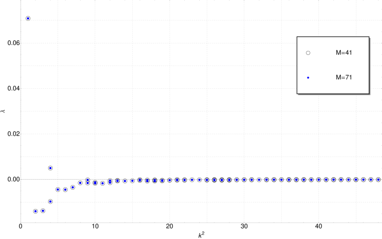
Figure 1: Eigenvalues $\lambda_{k}=\lambda_{k}^{(g)}+f\lambda_{k}^{(o)}$ as a function of $k^{2}$ for the massless overlap Dirac operator with $f=1$ and $m_{w}=-1$ obtained using numerical integration with $M^{4}$ equally spaced points in the four-dimensional integration space.

As a second example, we set $f=2$, keeping $m_{o}=0$ and $m_{w}=-1$. In this case, we find all eigenvalues $\lambda_{k}$ to be negative, making this a point inside the allowed region. In Fig. 2, we have plotted $\ln(-\lambda_{k})$ as a function of $k^{2}$ to show that even in the log-scale we have a good estimate for the continuum integral.

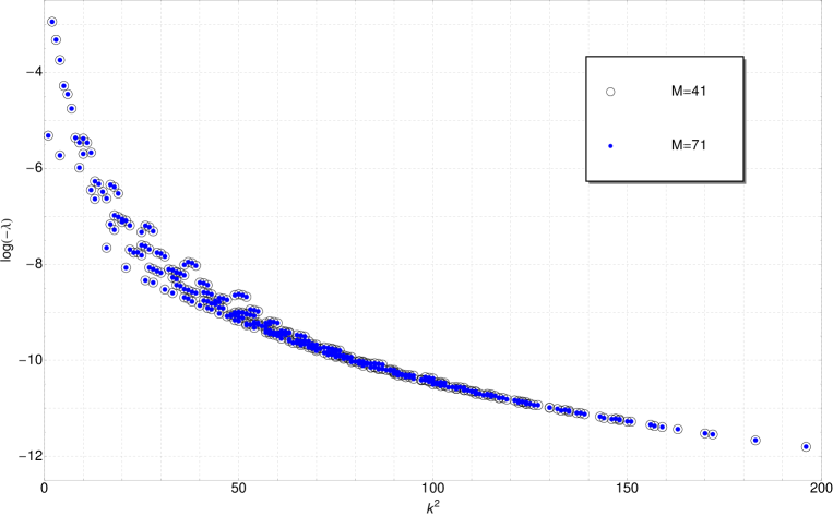
Figure 2: Logarithm of the eigenvalues for the massless overlap Dirac operator with $f=2$ and $m_{w}=-1$ obtained using numerical integration with $M^{4}$ equally spaced points in the four-dimensional integration space.

Numerically, we find that $\lambda_{k}^{(g)}>0$ for all $k$, which means that a point $(f,m_{o},m_{w})$ will be inside the allowed region (defined by $\lambda_{k}=\lambda_{k}^{(g)}+f\lambda_{k}^{(f)}<0$ for all $k$) iff

1. $\lambda_{k}^{(o)}(m_{o},m_{w})<0$ for all $k$,

2. $f>\max_{k}\left\{-\lambda^{(g)}_{k}/\lambda^{(o)}_{k}\right\}$.

We observe that the eigenvalues $\lambda_{k}^{(g)}$ and $\lambda_{k}^{(o)}$ go to zero as $k\to\infty$. As they approach zero from opposite sides ($\lambda^{(g)}>0$, $\lambda^{(o)}<0$), we potentially have to consider all $k$ in order to be able to determine the boundary of the allowed region in the $(f,m_{o},m_{w})$ space.

Let us first consider the case $m_{o}=0$. As $k\to\infty$, the integrals determining the eigenvalues in (25) are dominated by $\phi_{\nu}\in(0,2\pi/k_{\nu}]$ since both $S_{g}$ and $S_{o}$ diverge as $\phi\to 0$. Furthermore, expanding $S(\phi)$ around $\phi=0$, we obtain

$$S_{g}(\phi)=-\ln(\phi^{2})+\ldots\,;\qquad\qquad S_{o}(\phi)=2\ln(\phi^{2})+\ldots\,,$$ (29)

indicating that $-\lambda^{(g)}_{k}/\lambda^{(o)}_{k}\to\frac{1}{2}$ as $k\to\infty$ for all $m_{w}<0$. Computing the eigenvalues numerically, we indeed find that $-\lambda^{(g)}_{k}/\lambda^{(o)}_{k}$ rapidly converges to $\frac{1}{2}$ for large $k$ (cf. Fig. 3 for an example). Therefore, for $m_{o}=0$, the allowed region in the $(m_{w},f)$-plane is determined by eigenvalues $\lambda_{k}$ with $k$ being small (cf. Fig. 3). Considering only $f\leq\frac{11}{4}$, we find numerically that the maximum $-\lambda^{(g)}_{k}/\lambda^{(o)}_{k}$, which leads to the boundary of the allowed region, is obtained at $k=(2,2,2,2)$ for $m_{w}\in[-1.21,-1.15]$, at $k=(1,0,0,0)$ for $m_{w}\in[-1.15,-0.843]$, and at $k=(2,0,0,0)$ for $m_{w}\in[-0.843,-0.780]$. $m_{w}\notin[-1.21,-0.780]$ is not allowed. For a plot of the boundary of the allowed region in the $(m_{w},f)$-plane for $m_{o}=0$ see Fig. 4.

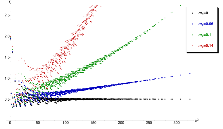
Figure 3: Plots of $f_{0}\equiv-\lambda^{(g)}_{k}/\lambda^{(o)}_{k}$ (for $k_{\mu}\leq 9$) at $m_{w}=-1$ and different choices for $m_{o}$. For $m_{o}=0$, $f_{0}\to 0.5$ as $k^{2}\to\infty$; for all $m_{o}>0$, $f_{0}\to\infty$ as $k^{2}\to\infty$. The boundary of the allowed region is determined by $\max_{k}f_{0}(k)$.

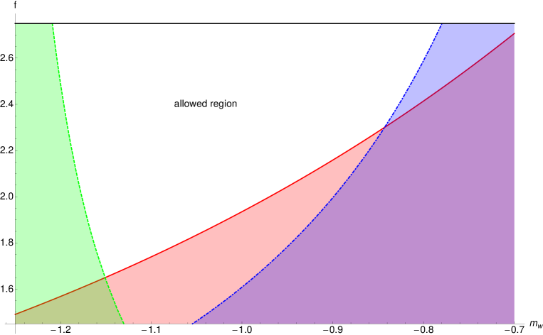
Figure 4: Boundary of the allowed region in the $(m_{w},f)$-plane for massless overlap fermions ($m_{o}=0$). The different lines show $-\lambda^{(g)}_{k}/\lambda^{(o)}_{k}$ for $k=(2,2,2,2)$ (green, dashed), $k=(1,0,0,0)$ (red, solid), and $k=(2,0,0,0)$ (blue, dot-dashed). The intersection points are at $(m_{w},f)\approx(-0.843,2.30)$ and $(m_{w},f)\approx(-1.15,1.65)$.

For $m_{o}>0$, the divergence of $S_{o}(\phi)$ at $\phi=0$ is regulated and therefore $\lambda_{k}^{(o)}(m_{o})/\lambda_{k}^{(o)}(m_{o}=0)\to 0$ as $k\to\infty$. Fig. 5 shows some examples for the dependence of $\lambda_{k}^{(o)}(m_{o})$ on $m_{o}$ and $k$ at $m_{w}=-1$. Together with our results for the massless case, this immediately implies that $-\lambda^{(g)}_{k}/\lambda^{(o)}_{k}\to\infty$ as $k\to\infty$ (see Fig. 3 for numerical results). Therefore, it is necessary to keep $m_{0}=0$ in the weak-coupling limit.

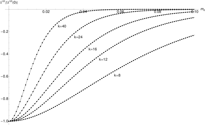
Figure 5: Plots of $\lambda_{k}^{(o)}(m_{o})/|\lambda_{k}^{(o)}(m_{o}=0)|$ at $m_{w}=-1$ for modes with $k_{\mu}=k\ \forall\mu$ and different choices of $k$. The ratio goes to zero as $k\to\infty$ for every $m_{o}>0$, with the rate of convergence increasing with $m_{o}$.

IV.2 Wilson fermions

The scenario for Wilson fermions is very similar to the overlap case described above, with $m_{w}$ now playing the role of $m_{o}$ and no additional irrelevant parameter. For $m_{w}=0$, we have $S_{w}(\phi)=2\ln(\phi^{2})+\ldots$ for small $\phi$, and therefore $-\lambda^{(g)}_{k}/\lambda^{(w)}_{k}\to\frac{1}{2}$ as $k\to\infty$, while for $m_{w}>0$, we find $-\lambda^{(g)}_{k}/\lambda^{(w)}_{k}\to\infty$ as $k\to\infty$, which means that $m_{w}>0$ is not allowed. Some numerical results are shown in Figs. 6 and 7, which directly correspond to Figs. 3 and 5 for the overlap case. For $m_{w}=0$, the maximum $-\lambda^{(g)}_{k}/\lambda^{(w)}_{k}$ is obtained at $k=(1,1,1,1)$, for which $-\lambda^{(g)}_{k}/\lambda^{(w)}_{k}=2.39$ (cf. Fig. 6). Therefore, only $m_{w}=0$ and $f>2.39$ is allowed for Wilson fermions in the weak-coupling limit.

Figure 6: Plots of $f_{0}\equiv-\lambda^{(g)}_{k}/\lambda^{(w)}_{k}$ (for $k_{\mu}\leq 9$) for different choices of $m_{w}$. For $m_{w}=0$, $f_{0}\to 0.5$ as $k^{2}\to\infty$; for $m_{w}>0$, $f_{0}\to\infty$ as $k^{2}\to\infty$.

Figure 7: Plots of $\lambda_{k}^{(w)}(m_{w})/|\lambda_{k}^{(w)}(m_{w}=0)|$ for modes with $k_{\mu}=k\ \forall\mu$ and different choices of $k$.

V Approach to the infinite-$N$ limit

Given the leading-order partition function in (13), we view the action as a function of the $4N$ angles subject to the condition that they belong to $\operatorname{SU}(N)$ and perform a maximization of the action using the Hybrid Monte Carlo algorithm as described in Hietanen:2009ex . Instead of looking at the distribution of the angles which can look uniform due to the action being invariant under $\theta_{\mu}^{i}\to\theta_{\mu}^{i}+\frac{2\pi k_{\mu}}{N}$ for arbitrary integers $k_{\mu}$, we look at the action $S^{0}$ and compare to what one would get if we replace $\rho(\theta)$ by the constant distribution $\frac{1}{(2\pi)^{4}}$ in (22) which we will be $N^{2}\lambda_{0}$. If the distributions at finite $N$ given by (17) for the maximum action configurations approach the uniform distribution as $N\to\infty$, we expect the action density, $s^{0}=\frac{S^{0}}{N^{2}}$, to approach $\lambda_{0}$. The plots in the top left panel of Fig. 8 are for two points in the allowed region and there is evidence for $s^{0}$ approaching $\lambda_{0}$ as $N\to\infty$. Contrary to this result, we see that $s^{0}$ does not approach $\lambda_{0}$ for two points outside the allowed region shown in the top right panel where we have only changed $f$ and kept $m_{w}=-1$ compared to the points shown in the top left panel. The bottom panel shows two other cases outside the allowed region where the parameters coincide with previous numerical work Hietanen:2012ma .

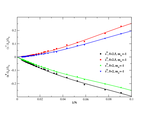
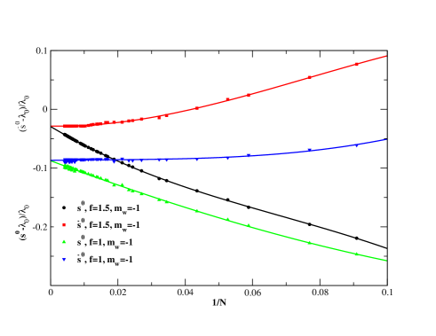
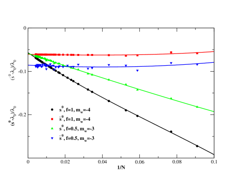
Figure 8: Approach of the lattice action density to the large-$N$ limit. The left panel shows that we approach a uniform distribution in the allowed region. The right panel shows that we do not approach a uniform distribution in the region that is not allowed. The bottom panel shows two other cases where we do not approach a uniform distribution in the region that is not allowed (note that $\lambda_{0}<0$, i.e., $\lim_{N\to\infty}s^{0}>\lambda^{0}$).

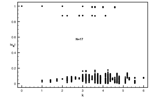
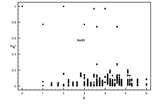
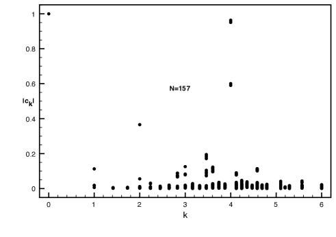
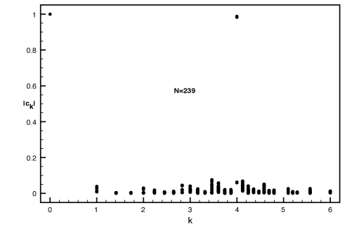
Figure 9: The Fourier coefficients, $|c_{k}|$, of $\rho(\theta)$ as a function of $k=\sqrt{k^{2}}$ for several values of $N$ with $f=2$ flavors of massless overlap fermions and the Wilson mass parameter set to $m_{w}=-1$.

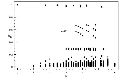
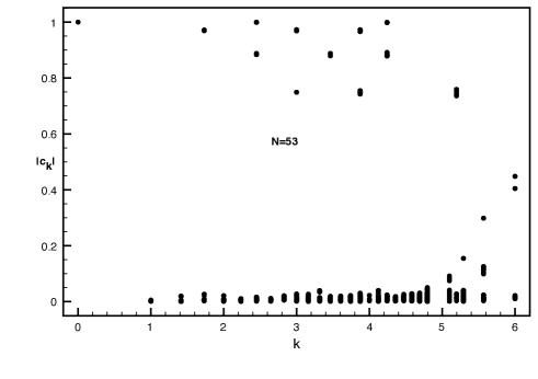
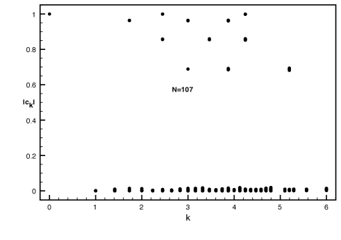
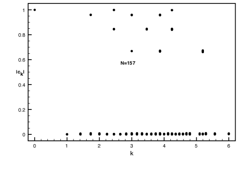
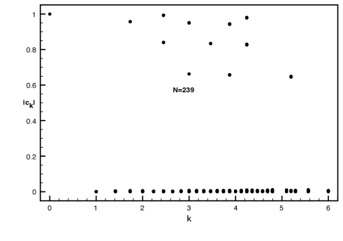
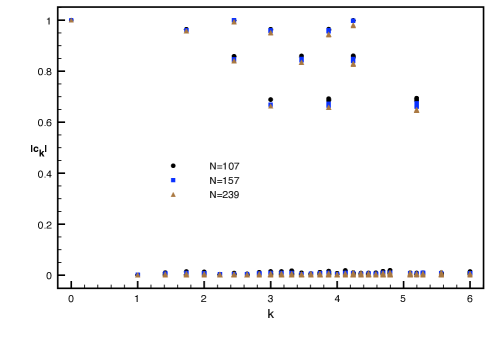
Figure 10: The Fourier coefficients, $|c_{k}|$, of $\rho(\theta)$ as a function of $k=\sqrt{k^{2}}$ for several values of $N$ with $f=1$ flavors of massless overlap fermions and the Wilson mass parameter set to $m_{w}=-4$.

In order to provide further support for the argument in the previous paragraph, we will start with the distribution at finite $N$ as given in (17) for the maximum action configuration $\{\theta_{\mu}^{i}\}$ and compute all Fourier coefficients

$$c_{k}=\int\prod_{\mu}d\theta_{\mu}\rho(\theta)e^{-i\sum_{\nu}k_{\nu}\theta_{\nu}}=\frac{1}{N}\sum_{j=1}^{N}e^{-i\sum_{\nu}k_{\nu}\theta_{\nu}^{j}}=\frac{1}{N}\operatorname{Tr}\left(\prod_{\nu}D_{\nu}^{k_{\nu}}\right)^{\dagger}$$ (30)

for all $k$ with $-3\leq k_{\mu}\leq 3$. The results for several values of $N$ for one point in the allowed region ($f=2$, $m_{o}=0$, $m_{w}=-1$) that coincides with a point in the top left panel of Fig. 8 are shown in Fig. 9. Results for one point outside the allowed region ($f=1$, $m_{o}=0$, $m_{w}=-4$) that coincides with a point in the bottom panel of Fig. 8 are shown in Fig. 10. We expect all the Fourier coefficients shown in Fig. 9 to approach zero and there is some evidence for this. We can imagine constructing a sequence of distributions for $N=n^{4}$ (with $n=2,3,\ldots$) that approaches a uniform distribution in the large-$N$ limit by locating $\delta$-functions on all sites of a four-dimensional periodic hypercubic lattice with lattice spacing $2\pi/n$. The corresponding Fourier coefficients $c_{k}$ would by $1$ if all $k_{\mu}$ are multiplies of $n$ and zero otherwise. It is therefore not surprising that we obtain non-zero Fourier coefficients $c_{k}$ with $k$ being of order $N^{\frac{1}{4}}$ in Fig. 9 even though we expect all coefficients to vanish in the large-$N$ limit.

On the other hand, we expect some of the Fourier coefficients shown in Fig. 10 to approach a non-zero limit and there is some evidence for this particularly when we look at the combined plot for $N=107,157,239$ shown in the bottom right panel.

If some of the Fourier coefficients shown in Fig. 10 indeed approach a non-zero limit, the partial continuum action density defined as

$$\bar{s}^{0}=\sum_{|k_{\mu}|\leq 3}c_{k}c_{k}^{*}\lambda_{k}\,,$$ (31)

should not approach $\lambda_{0}$. There is clear evidence for it when we look at the plots in the top right and bottom panels of Fig. 8. Note that the approach to $N\to\infty$ is quite flat consistent with the convergence seen in the combined plot for $N=107,157,239$ shown in the bottom right panel. Furthermore, the limit of $s^{0}$ and $\bar{s}^{0}$ do not seem to coincide in the bottom panel of Fig. 8 for the case of $f=0.5$ and $m_{w}=-3$ suggesting that there are modes with $k$ not in $-3\leq k_{\mu}\leq 3$ that approach a non-zero limit at infinite $N$.

Only in the limit of infinite $N$, we are allowed to ignore the restriction of the principal value and sum the infinite series in (27) to obtain a finite action density provided the distribution has a smooth limit. The partial sum $\bar{s}^{0}$, on the other hand, is finite at any $N$ but will only agree with $s^{0}$ at infinite $N$ if all the coefficients not included in the sum approach zero excluding some accidental cancellation due to eigenvalues with different signs. If the distribution is uniform in the infinite-$N$ limit as is expected for points in the allowed region, we expect $s^{0}$ and $\bar{s}^{0}$ to coincide with $\lambda_{0}$. There is evidence for this in the top left panel of Fig. 8.

The computation of $\lambda_{k}$ in (25) should exclude a small region of order $\epsilon$ around $\phi=0$ in order to properly account for the principal value required at finite $N$ due to the form of the distribution in (17). One has to tune $\epsilon$ as a function of $N$ and include a sum over all modes in (27) (which will be finite) to match with $s^{0}$ at finite $N$. The difference between $s^{0}$ and $\bar{s}^{0}$ at finite $N$ seen in Fig. 8 is a combination of two effects: not excluding a small region of order $\epsilon$ and not including a sum over all modes.

VI Discussion of previous numerical work

Previous numerical work described in Hietanen:2009ex only looked at one Fourier mode, namely, $k_{\mu}=(1,0,0,0)$ and its permutations. We know from the analysis of the Fourier modes in this paper, that some coefficients could be accidentally small and it is necessary to look at several Fourier modes. The wilson mass parameter was set to $m_{w}=-5$ in the numerical analysis performed in Hietanen:2009ex at finite lattice coupling and we know from the analysis performed here that this is not in the allowed region for any value of $f$ in the weak-coupling limit.

Numerical work in Hietanen:2012ma falls under a slightly different category. The running of the coupling studied in that paper at the range of lattice couplings did not agree with two loop perturbation theory. Since the theory studied used massless overlap fermions with $f=1$ and $m_{w}=-4$, we know from the analysis performed here that we cannot obtain an infinite-volume continuum limit by going to $b\to\infty$ (weak-coupling limit). The speculative part in Hietanen:2012ma suggests the possibility of a continuum limit away from $b=\infty$. If this is the case, then the analysis performed in this paper does not shed light into such a scenario.

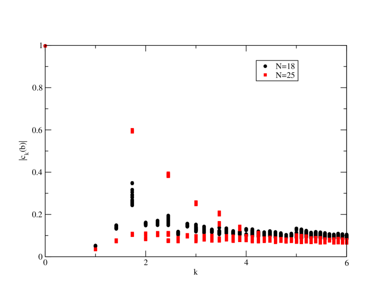
Figure 11: The Fourier coefficents, $c_{k}(b),$ as a function of $k=\sqrt{k^{2}}$ at finite lattice coupling, $b=0.65,$ with one flavor of massless overlap Dirac fermions and $m_{w}=-4$.

Numerical studies with two flavors of Wilson fermions (both massless and massive) were carried out in Bringoltz:2011by . From Fig. 6 in this paper, we know that we cannot obtain the infinite-volume continuum limit with one or two flavors of Wilson fermions. Evidence for being in the correct continuum phase was obtained by a study of operators of the form $|\operatorname{Tr}U_{\mu}|$, $|\operatorname{Tr}U_{\mu}U_{\nu}|$ and $|\operatorname{Tr}U_{\mu}U_{\nu}^{\dagger}|$. These can be considered as special cases of

$$c_{k}(b)=\operatorname{Tr}U_{1}^{k_{1}}U_{2}^{k_{2}}U_{3}^{k_{3}}U_{4}^{k_{4}}$$ (32)

which will tend to $c_{k}$ in (30) in the weak-coupling limit, $b\to\infty$. The ordering of the operators will matter at finite lattice coupling if more than two of the $k_{\mu}$ are non-zero. We do not have the gauge field data for Wilson fermions used in Bringoltz:2011by but we do have them for massless overlap fermions at $b=0.65$, $f=1$ and $m_{w}=-4$ in Hietanen:2012ma . The results for $c_{k}(b)$ are plotted in Fig. 11 and should be compared with Fig. 10. We see that $b=0.65$ is far away from the weak-coupling limit consistent with the results in Hietanen:2012ma . Furthermore, the coefficients with small $k$ could be accidentally small. This suggests that the conclusions in Bringoltz:2011by possibly result from being far away from the weak-coupling limit and not looking at a sufficient number of Fourier modes.

In addition, we can also conclude that we cannot use a single-site model with heavy Wilson fermions and obtain the continuum limit of a pure gauge theory in contrast to the claims made in Hanada:2013ota . The eigenvalues of Wilson fermions are doubly degenerate Hietanen:2009ex but they do not come in pairs of opposite chirality. Therefore, it is not apriori clear how to deal with half a flavor of Wilson fermions making it essentially impossible to study the continuum limit of any infinite-volume theory using adjoint Wilson fermions on a single-site lattice.

Since we cannot keep the bare mass finite and non-zero as we take the weak-coupling limit, the proposal in Azeyanagi:2010ne to use single-site models with massive adjoint fermions in order to extract physics of pure gauge theories is ruled out.

VII Future Work

The allowed regions plotted in Fig 4 provide for an interesting scenario when it comes to the usefulness of single-site theories to describe correct infinite-volume continuum physics. We cannot study theories with $f\leq\frac{3}{2}$ unless we entertain the possibility that the continuum limit occurs away from $b=\infty$ but this would be a radical deviation from conventional wisdom. We can study $f\geq 2$ theories without a fermion mass. It is possible we can study $f\geq 2$ theories with a fermion mass provided we can stay in the correct phase by taking the bare mass to zero as we go to the weak-coupling limit such that the physical mass is kept constant. Since this theory is expected to be conformal for massless fermions, it is not clear how a single-site theory will exhibit conformal behavior. This is certainly a case worth further investigation.

- (1) A. Hasenfratz, A. Cheng, G. Petropoulos and D. Schaich, arXiv:1303.7129 [hep-lat].
- (2) B. Svetitsky, arXiv:1301.1877 [hep-lat].
- (3) Y. Iwasaki, arXiv:1212.4343 [hep-lat].
- (4) G. Petropoulos, A. Cheng, A. Hasenfratz and D. Schaich, PoS LATTICE 2012, 051 (2012) [arXiv:1212.0053 [hep-lat]].
- (5) T. DeGrand, Y. Shamir and B. Svetitsky, Phys. Rev. D 85, 074506 (2012) [arXiv:1202.2675 [hep-lat]].
- (6) T. DeGrand, Phys. Rev. D 84, 116901 (2011) [arXiv:1109.1237 [hep-lat]].
- (7) G. Voronov [LSD Collaboration], PoS LATTICE 2011, 093 (2011).
- (8) A. Patella, L. Del Debbio, B. Lucini, C. Pica and A. Rago, PoS LATTICE 2011, 084 (2011) [arXiv:1111.4672 [hep-lat]].
- (9) S. Catterall, L. Del Debbio, J. Giedt and L. Keegan, Phys. Rev. D 85, 094501 (2012) [arXiv:1108.3794 [hep-ph]].
- (10) Z. Fodor, K. Holland, J. Kuti, D. Nogradi and C. Schroeder,
- (11) S. Catterall, J. Giedt, F. Sannino and J. Schneible, arXiv:0910.4387 [hep-lat].
- (12) T. Appelquist, G. T. Fleming and E. T. Neil, Phys. Rev. D 79, 076010 (2009) [arXiv:0901.3766 [hep-ph]].
- (13) A. Hietanen, J. Rantaharju, K. Rummukainen and K. Tuominen, PoS LATTICE 2008, 065 (2008) [arXiv:0810.3722 [hep-lat]].
- (14) T. Appelquist, G. T. Fleming and E. T. Neil, Phys. Rev. Lett. 100, 171607 (2008) [Erratum-ibid. 102, 149902 (2009)] [arXiv:0712.0609 [hep-ph]].
- (15) P. Kovtun, M. Unsal, L. G. Yaffe, JHEP 0706, 019 (2007). [hep-th/0702021 [HEP-TH]].
- (16) P. F. Bedaque, M. I. Buchoff, A. Cherman and R. P. Springer, JHEP 0910, 070 (2009) [arXiv:0904.0277 [hep-th]].
- (17) B. Bringoltz, JHEP 0906, 091 (2009). [arXiv:0905.2406 [hep-lat]].
- (18) B. Bringoltz and S. R. Sharpe, Phys. Rev. D 80, 065031 (2009) [arXiv:0906.3538 [hep-lat]].
- (19) E. Poppitz, M. Unsal, JHEP 1001, 098 (2010). [arXiv:0911.0358 [hep-th]].
- (20) A. Hietanen, R. Narayanan, JHEP 1001, 079 (2010). [arXiv:0911.2449 [hep-lat]].
- (21) T. Azeyanagi, M. Hanada, M. Unsal, R. Yacoby, Phys. Rev. D82, 125013 (2010). [arXiv:1006.0717 [hep-th]].
- (22) S. Catterall, R. Galvez, M. Unsal, JHEP 1008, 010 (2010). [arXiv:1006.2469 [hep-lat]].
- (23) A. Hietanen, R. Narayanan, Phys. Lett. B698, 171-174 (2011). [arXiv:1011.2150 [hep-lat]].
- (24) B. Bringoltz, M. Koren, S. R. Sharpe, [arXiv:1106.5538 [hep-lat]].
- (25) A. Hietanen and R. Narayanan, Phys. Rev. D 86, 085002 (2012) [arXiv:1204.0331 [hep-lat]].
- (26) M. Hanada, J. -W. Lee and N. Yamada, arXiv:1302.3532 [hep-lat].
- (27) A. Gonzalez-Arroyo and M. Okawa, PoS LATTICE 2012, 046 (2012) [arXiv:1210.7881 [hep-lat]].
- (28) A. González-Arroyo and M. Okawa, arXiv:1304.0306 [hep-lat].
- (29) G. Bhanot, U. M. Heller and H. Neuberger, Phys. Lett. B 113, 47 (1982).