Quantisation of the effective string with TBA

Abstract:

In presence of a static pair of sources, the spectrum of low-lying states of whatever confining gauge theory in D space-time dimensions is described, at large source separations, by an effective string theory. In the far infrared the latter flows, in the static gauge, to a two-dimensional massless free-field theory. It is known that the Lorentz invariance of the gauge theory fixes uniquely the first few subleading corrections of this free-field limit. We point out that the first allowed correction - a quartic polynomial in the field derivatives - is exactly the composite field $T\bar{T}$, built with the chiral components, $T$ and $\bar{T}$, of the energy-momentum tensor. This irrelevant perturbation is quantum integrable and yields, through the thermodynamic Bethe Ansatz (TBA), the energy levels of the string which exactly coincide with the Nambu-Goto spectrum. We obtain this way the results recently found by Dubovsky, Flauger and Gorbenko. This procedure easily generalizes to any two-dimensional CFT. It is known that the leading deviation of the Nambu-Goto spectrum comes from the boundary terms of the string action. We solve the TBA equations on an infinite strip, identify the relevant boundary parameter and verify that it modifies the string spectrum as expected.

1 Introduction

Even though a rigorous proof of quark confinement in Yang-Mills theories is still missing, numerical experiments and theoretical arguments leave little doubt that this phenomenon is associated to the formation of a thin string-like flux tube, the confining string, which generates, for large quark separations, a linearly rising of confining potential.

The string-like nature of the flux tube is particularly evident in the strong coupling region of lattice gauge theories, where the vacuum expectation value of large Wilson loops is given by a sum over certain lattice surfaces which can be considered as the world-sheet of the underlying confining string. When the coupling constant decreases, this two-dimensional system undergoes a roughening transition [1] where the sum of these surfaces diverges and the colour flux tube of whatever lattice gauge theory undergoes a transition towards a rough phase, which is connected to the continuum limit. It is widely believed that such a phase transition belongs to the Kosterlitz-Thouless universality class [2]. Accordingly, the renormalisation group equations imply that the effective string action $S$ describing the dynamics of the flux tube in the whole rough phase flows at large scales towards a massless free-field theory. Thus, for large enough inter-quark separations it is not necessary to know explicitly the specific form of the effective string action $S$, but only its infrared limit

$$S[X]=S_{cl}+S_{0}[X]+\dots,$$ (1)

where the classical action $S_{cl}$ describes the usual perimeter-area term, $X$ denotes the two-dimensional bosonic fields $X_{i}(\xi_{1},\xi_{2})$, with $i=1,2,\dots,D-2$, describing the transverse displacements of the string with respect the configuration of minimal energy, $\xi_{1},\xi_{2}$ are the coordinates on the world-sheet and $S_{0}[X]$ is the Gaussian action

$$S_{0}[X]=\frac{\sigma}{2}\int d^{2}\xi\left(\partial_{\alpha}X\cdot\partial^{\alpha}X\right)~{}.$$ (2)

This action is written in the physical or static gauge, where the only degrees of freedom taken into account are the physical ones i.e. the transverse displacements $X_{i}$. Even in this infrared approximation the effective string is highly predictive, indeed it predicts the leading correction to the linear quark-anti-quark potential, known as Lüscher term [3, 4]

$$V(R)=\sigma R-\frac{\pi(D-2)}{24R}+O(1/R^{2})~{}.$$ (3)

Accurate numerical simulations have shown the validity of that expectation [5, 6, 7, 8, 9, 10]. This infrared limit also accounts for the logarithmic broadening of the string width as a function of the inter-quark separation [11]. This phenomenon was first observed long time ago in the $\mathbb{Z}_{2}$ 3D gauge theory [12] and only recently, using the very efficient Lüscher-Weisz algorithm [9], has also been observed in a non-abelian Yang-Mills theory [13, 14].

In the last few years there has been a substantial progress in lattice simulations in measuring various properties of the flux tube, in particular the interquark potential and the energy of the excited string states (see e.g. [15, 16, 17, 18, 19, 20, 21, 22, 23, 24, 25, 26]) which is now sensible to the first few subleading corrections of the free-field infrared limit of the effective action. The latter is the sum of all the terms respecting the symmetry of the system, which in an Euclidean space is $SO(2)\times ISO(D-2)$. The first few terms are

$$S=S_{cl}+S_{0}[X]+\sigma\int d^{2}\xi\left[c_{2}(\partial_{\alpha}X\cdot\partial^{\alpha}X)^{2}+c_{3}(\partial_{\alpha}X\cdot\partial^{\beta}X)(\partial_{\beta}X\cdot\partial^{\alpha}X)\right]+S_{b}+\dots~{},$$ (4)

where $S_{b}$ is the boundary action characterizing the open string. Indeed quantum field theories on space-time manifolds with boundaries require, in general, the inclusion in the action of contributions localized at the boundary. If the boundary is a Polyakov line in the $\xi_{0}$ direction, on which we assume Dirichlet boundary conditions, the first few terms are

$$S_{b}=\int d\xi_{0}\left[b_{1}(\partial_{1}X\cdot\partial_{1}X)+b_{2}(\partial_{1}\partial_{0}X\cdot\partial_{1}\partial_{0}X)+b_{3}(\partial_{1}X\cdot\partial_{1}X)^{2}+\dots\right]\,.$$ (5)

Of course the addition of these terms modifies the spectrum of the physical states. For instance the interquark potential (3) becomes, at first order in $b_{1}$ [9],

$$V(R)=\sigma R-\frac{\pi(D-2)}{24R}-b_{1}\frac{\pi(D-2)}{6R^{2}}+O(1/R^{3})~{}.$$ (6)

In 2004 Lüscher and Weisz [27] noted that the comparison of the string partition function on a cylinder (Polyakov correlator) with the sum over closed string states in a Lorentz (or rotation) invariant theory yields strong constraints (called open-closed string duality). In particular they showed in this way that $b_{1}=0$. This property was then further generalized in [28]. It was subsequently recognized that an essential ingredient of these constraints is the Lorentz invariance of the bulk space-time [29, 30, 31]. The confining string action could be regarded as the effective action obtained from the underlying Yang-Mills theory of the confining vacuum in presence of a large Wilson loop by integrating out all the massive degrees of freedom [31]. This integration does not spoil the original Poincaré invariance of the underlying gauge theory, however this symmetry is no longer manifest, being spontaneously broken. As expected, it is realized through non-linear transformations of the $X^{i}$’s. The effective string action (4) should be invariant under the infinitesimal Lorentz transformation in the plane $(\alpha,j)$

$$\delta X^{i}=-\epsilon^{\alpha j}\delta^{ij}\xi_{\alpha}-\epsilon^{\alpha j}X_{j}\partial_{\alpha}X^{i}\,.$$ (7)

For instance, if we apply the transformation (7) to the term $S_{b_{1}}$ proportional to $b_{1}$ in the boundary action $S_{b}=S_{b_{1}}+S_{b2}+\dots$ we get at once

$$\delta(S_{b_{1}})=-b_{1}\int\epsilon^{1i}d\xi_{0}\,\partial_{1}X_{i}+{\rm higher~{}order~{}terms~{}}\not=0\,,$$ (8)

thus such a term breaks explicitly Lorentz invariance, hence $b_{1}=0$. In a similar way [31] it is possible to show that $b_{3}=0$ . On the contrary the $b_{2}$ term is compatible with Lorentz invariance provided we add an infinite sequence of terms generated by the non-linearity of the transformation. The associated recursion relations can be easily solved and the final expression can be written in a closed form [32]

$$S_{2}=b_{2}\int d\xi_{0}\left[\frac{\partial_{1}\partial_{0}X\cdot\partial_{1}\partial_{0}X}{1+\partial_{1}X\cdot\partial^{1}X}+\frac{(\partial_{1}\partial_{0}X\cdot\partial_{1}X)^{2}}{(1+\partial_{1}X\cdot\partial^{1}X)^{2}}\right]\,.$$ (9)

It is easy to construct in this way boundary terms of higher order [32]. Actually this procedure was first applied to the bulk action and it was shown that the requirement of Lorentz invariance of the infrared free-field limit (1) generates the whole Nambu-Goto (NG) action [30, 31, 33]. In the latter reference this method was generalized to the construction of the effective action of higher dimensional extended objects as D-branes on which other massless modes, besides the $X^{i}$’s, are propagating. It can also be used to construct the allowed bulk corrections to the Nambu-Goto action [34, 35, 36]; further informations on the bulk corrections of the NG can be found working in a gauge where the Lorentz invariance is manifest [37, 38] (see also a general discussion on this argument in [39]).

A formal light-cone quantisation of the Nambu-Goto action [40] suggested a simple Ansatz for the energy spectrum of the closed string of length $R$

$$E_{(n,\bar{n})}(R)=\sqrt{\sigma^{2}R^{2}+4\pi\sigma\left(n+\bar{n}-\frac{D-2}{12}\right)+\left(\frac{2\pi(n-\bar{n})}{R}\right)^{2}}\,,$$ (10)

where the integers $n,\bar{n}$ define the total energy $2\pi n/R$ $(2\pi\bar{n}/R)$ of the left (right) moving massless phonons. Similarly for the open string with fixed ends, where $n=\bar{n}$, one has

$$E_{n}(R)=\sqrt{\sigma^{2}R^{2}+2\pi\sigma\left(n-\frac{D-2}{24}\right)}\,.$$ (11)

We refer to (10) and (11) as the exact Nambu-Goto spectrum even if we know that this Ansatz is incompatible with Lorentz invariance in $D<26$ [41], except maybe in $D=3$ [42].

For large enough $R$ one can expand (10) and (11) in powers of $1/\sigma R^{2}$. Lattice simulations of confining gauge theories in 2+1 and 3+1 dimensions show that the ground state and the first excitations of the confining string have an energy spectrum very close to that of NG. This suggests that the effective action constructed along the lines illustrated above can be considered as small perturbations of NG action that can be evaluated using a suitable regularization and a standard expansion in perturbative diagrams [27, 43]. It turns out that only first order calculations on the parameters $c_{i}$ and $b_{i}$ are practically feasible.

Recently, a new powerful non-perturbative method has been introduced in this context [38]. It is based on the study of the $S$ matrix describing the scattering of the quanta of the string excitations, the phonons, in the word-sheet. Assuming a reasonably simple form for $S$ it turns out that the system is quantum integrable [44], hence one can apply the method of thermodynamic Bethe Ansatz (TBA) to calculate the non-perturbative spectrum of the effective string. Taking the simplest form of the $S$ matrix and some assumptions on the way of interacting of the phonons with different flavours (i.e. transverse indices), it turns out the spectrum coincides with the exact NG spectrum of the closed string [44]. This method was also applied to describe some apparent deviations of the spectrum of the closed string [45].

In the present paper we re-derive the NG spectrum starting from the observation that the first non-Gaussian correction of the string action (4), once the coefficients $c_{i}$ assume the values required by Lorentz invariance of the target space, namely $c_{2}=\frac{1}{8}$ and $c_{3}=-\frac{1}{2}$, coincide with the composite field $T\bar{T}$, where $T$ and $\bar{T}$ are the chiral components of the energy momentum tensor $T_{\alpha\beta}$. Thus the effective string action is, at this perturbative order, a two-dimensional integrable quantum field theory formed by a conformal field theory (the infrared Gaussian limit) perturbed by $T\bar{T}$. We do not need any further assumption to derive, through the TBA, the NG spectrum.

We also show that a similar spectrum emerges from a general class of CFT’s perturbed by $T\bar{T}$. The energy levels for the identity primary field and its descendents coincides with (10) and (11) once one replaces $D-2$ with the central charge $c$. The level degeneracy differs in an intriguing way: it is know that the degeneracy of the closed string grows exponentially for large $E$ as $\sim\exp(E/T_{H})$, where $T_{H}=\sqrt{3\sigma/\pi(D-2)}$ -the Hagedorn temperature- coincides with the inverse of the distance $R_{c}$ where the ground state of the NG spectrum develops a tachyon, i.e. where the argument of the square root in (10) vanishes. A similar relationship between the position of the tachyonic singularity of the ground state and the degeneracy of highly excited states holds for general CFT’s. We shall check it in the critical Ising model where this degeneracy can be calculated exactly.

The interplay between quantum integrability and Lorentz invariance in the target space is an intriguing issue: the first non-Gaussian contribution of the string action is an integrable perturbation only if $c_{2}/c_{3}=-\frac{1}{4}$ as required by Lorentz invariance, however this does not imply that the generated NG spectrum agrees with that of a Lorentz-invariant string theory. As already mentioned, a pure NG spectrum is compatible with Lorentz invariance in the Minkowski target space only for $D=26$ (and perhaps $D=3$) and perturbative calculations show that the NG spectrum deviates from that of a Lorentz-invariant string already at the order $1/R^{5}$ in $D>3$ dimensions , and starting at the order $1/R^{7}$ non-universal terms are expected to contribute to the energy levels [43, 38, 39]. These contributions could be inserted in the TBA approach by assuming that at shorter distances other perturbations contribute, besides $T\bar{T}$.

Actually the leading deviation of the NG spectrum comes from the boundary action (9). This is also the most significant from a phenomenological point of view, being associated with the first non-NG correction of the interquark potential. We have indeed [27, 43]

$$V(R)=\sigma R-\frac{\pi(D-2)}{24R}-\frac{1}{2\sigma R^{3}}\left(\frac{\pi(D-2)}{24}\right)^{2}-b_{2}\frac{\pi^{3}(D-2)}{60R^{4}}+O(1/R^{5})~{},$$ (12)

where the third term comes from the $c_{2}$ and $c_{3}$ terms in (4) [27]. This deviation of the interquark potential has been already observed in lattice gauge theories and the $b_{2}$ parameter has been evaluated [46, 32].

In this paper we introduce the TBA equations describing these boundary effects by generalizing the approach of [38] to an infinite strip with Dirichlet boundary conditions. We find that also in this case the equations are solvable explicitly and the energy spectrum is given by (11). It is also easy to derive the corrections of the open string NG spectrum due to the boundary constants $b_{i}$ and we recover in particular eq. (12).

Even though the non-perturbative method we used is very powerful and the calculations of the level corrections due to these coupling constants could be easily pushed to any perturbative order, we do not think that this formulation of the effective string is ultraviolet complete. The reason is that the whole spectrum of the theory includes an infinite set of negative energy levels: because of the square root in eq. (10), the complete energy spectrum is actually $\{\pm E_{(n,\bar{n})}(R)\}$. The theory can be fermionized and one may assume that the sea of negative energy levels is completely filled, however we did not succeeded in finding the zero-point energy produced by this sea, because of the huge degeneracy of the string states. As far as this problem is not completely solved, one should regard this formulation as an effective theory.

In the next Section we provide an elementary calculation of the $T\bar{T}$ nature of the quartic term along with some quantum check. In Section 3 we describe in detail the exact $S$ matrix for a critical RG flow of the Ising model in the limit of the massless phonons, following the method of Aliosha Zamoldchikov in the study of the flux between the tricritical Ising model and the critical Ising model and obtain the spectrum of the $T\bar{T}$ perturbed Ising model in a closed form. In Section 4 we study the degeneracy of the spectrum and compare it with the degeneracy of the string. Then in Section 5 we put the theory in an infinite strip, define a consistent reflection factor and, in Section 6, solve the boundary TBA for the open string in the case $D=3$ and compare it with the perturbative calculations. Finally, in Appendix A, we show that Nambu-Goto like spectra emerge from a large class of $T\bar{T}$ perturbed CFT’s and Section 7 contains our conclusions with a summary of the main results.

2 The composite perturbation $T\bar{T}$ and its expectation value

The energy-momentum tensor of the free-field theory (2) can be written as

$$T_{\alpha\beta}=\partial_{\alpha}X\cdot\partial_{\beta}X-\frac{1}{2}\delta_{\alpha\beta}\left(\partial^{\gamma}X\cdot\partial_{\gamma}X\right)\,.$$ (13)

Note that this tensor is symmetric, traceless and conserved, as it should. Once we put in eq. (4) the values of $c_{2}$ and $c_{3}$ prescribed by Lorentz invariance, we have, as anticipated in the Introduction,

$$S=S_{cl}+S_{0}[X]-\frac{\sigma}{4}\int d^{2}\xi\,T_{\alpha\beta}T^{\alpha\beta}+S_{b}+\dots$$ (14)

In two-dimensional CFT it is useful to introduce the chiral components $T_{zz}=\frac{1}{2}(T_{11}-iT_{12})$ and $T_{\bar{z}\bar{z}}=\frac{1}{2}(T_{11}+iT_{12})$ and use the normalized quantities $T=-2\pi\sigma T_{zz}$, $\bar{T}=-2\pi\sigma T_{\bar{z}\bar{z}}$ in such a way the operator product expansion begins with

$$T(z)T(w)=\frac{D-2}{2}\frac{1}{(z-w)^{4}}+\dots$$ (15)

and similarly for $\bar{T}$. Thus at the end we have

$$S=S_{cl}+S_{0}[X]-\frac{1}{2\pi^{2}\sigma}\int d^{2}\xi\,T\bar{T}+S_{b}+\dots$$ (16)

There is a consistency check based on some general properties of the expectation value of the composite field $T\bar{T}$ pointed out by Sasha Zamolodchikov [47] for any two-dimensional quantum field theory. In the particular case of a CFT on a infinite strip we have

$$\langle T\bar{T}\rangle=\langle T\rangle\langle\bar{T}\rangle\,.$$ (17)

Under a conformal mapping $z\to w=f(z)$, $T$ transforms as

$$T(z)=\left(\frac{df}{dz}\right)^{2}T(w)+\frac{c}{12}\{f,z\}\,,$$ (18)

where $\{f,z\}=-2\sqrt{f^{\prime}}\frac{d^{2}}{dz^{2}}\frac{1}{\sqrt{f^{\prime}}}$ is the Schwarzian derivative and $c$ the central charge.

Starting from the observation that $\langle T\rangle=0$ in the complex $w$ plane and that the transformation $f(z)=\exp(\pi z/R)$ maps conformally the infinite strip into the upper half plane $\Im m(w)\geq 0$, we get, as it is well known,

$$\langle T\rangle_{\rm strip}=\langle\bar{T}\rangle_{\rm strip}=\frac{c}{12}\{f,z\}=-\frac{c}{24}\left(\frac{\pi}{R}\right)^{2}\,,$$ (19)

therefore in the infinite strip limit $L\to\infty$ we should find

$$\int d^{2}\xi\,\langle T\bar{T}\rangle=RL\langle T\rangle^{2}_{\rm strip}\,.$$ (20)

On the other hand, the vacuum expectation value of the quartic term of the string action on a cylinder -i.e. the correlator of two Polyakov lines- has been calculated many years ago [48] in the $\zeta$-function regularization and more recently [27] in the dimensional regularization. The result is

$$-\frac{1}{2\pi^{2}\sigma}\int d^{2}\xi\,\langle T\bar{T}\rangle=-\frac{1}{2\pi^{2}\sigma}\frac{(D-2)\pi^{4}L}{24^{2}R^{3}}\left[(D-4)E_{2}(\tau)^{2}+2E_{4}(\tau)\right]\,,~{}\tau=i\frac{L}{2R}\,,$$ (21)

where $L$ is the circumference of the cylinder. We do not need the explicit expression of the Eisenstein series $E_{2}$ and $E_{4}$ because in the infinite strip limit $L\to\infty$ they become $E_{2}=E_{4}=1$. In this limit we recover eq. (20).

We conclude this Section with the following remark. The free-field action (14), once perturbed with $T\bar{T}$, has a new energy-momentum tensor which is no longer the one defined in (13) as it includes a quartic polynomial in the derivatives of $X_{i}$. Inserting this new $T\bar{T}$ perturbation generates a new energy-momentum tensor made with a polynomial of higher degree, and so on. It would be interesting to see whether this kind of recursion generates the same sequence produced by the request of Lorentz invariance in the target space.

3 The exact $S$ matrix for massless flows

More than twenty years ago, Aliosha Zamolodchikov [49] has proposed an interesting variant of the thermodynamic Bethe Ansatz [50] and the exact $S$ matrix approach to two-dimensional quantum field theory describing interpolating trajectories among pairs of nontrivial CFTs. The simplest instance discussed in [49], concerns the line of second order phase transitions connecting the tricritical Ising model (TIM) –identified with the conformal minimal model ${\cal M}_{4,5}$ perturbed by $\phi_{13}$– to the Ising model (IM). The latter system corresponding to the CFT ${\cal M}_{3,4}$ underlying the infrared fixed point of the RG flow.

Massless excitations confined on a infinite line or a ring naturally separate into right and left movers. In this simple example, only one species of particles is present. The right-right and left-left mover scattering is trivial, while the left-right scattering is described by the amplitude

$$S(p,q)=\frac{2\sigma+ipq}{2\sigma-ipq}~{},$$ (22)

where the real parameter $\sigma$ sets the scale; it plays the role of string tension in the energy spectrum. In (22) $p$ is the momentum of the right mover and $-q$ the momentum of the left mover. In the limit $\sigma\rightarrow\infty$, $S(p,q)\rightarrow 1$, right and left mover excitations decouple and the scale invariance of the model is fully restored at $\sigma=\infty$. Starting from the $S$ matrix (22), Zamolodchikov was then able to derive the thermodynamic Bethe Ansatz equations for the vacuum energy of the theory defined on a infinite cylinder with circumference $R$. The relevant equations are

$$\epsilon(p)=Rp-\int_{0}^{\infty}\frac{dq}{2\pi}\phi(p,q)\,\bar{L}(q),~{}~{}~{}\bar{\epsilon}(p)=Rp\ -\int_{0}^{\infty}\frac{dq}{2\pi}\phi(p,q)\,L(q)~{},$$ (23)

where $\epsilon(p)$ and $\bar{\epsilon}(p)$ are the pseudoenergies for the right and the left movers, respectively,

$$\phi(p,q)=-i\partial_{q}\text{ln}\;S(p,q)~{},$$ (24)

and

$$L(p)=\text{ln}(1+e^{-\epsilon(p)})~{},~{}~{}\bar{L}(p)=\text{ln}(1+e^{-\bar{\epsilon}(p)})~{}.$$ (25)

The ground state energy is

$$E^{(\text{TBA})}(R)=-\frac{\pi}{6R}c(\sqrt{\sigma}R)=-\int_{0}^{\infty}\frac{dp}{2\pi}(L(p)+\bar{L}(p))~{},$$ (26)

where $c(R\sqrt{\sigma})$ is the (flowing) effective central charge with

$$\text{c}_{\text{UV}}=c_{\text{TIM}}=c(0)=\frac{7}{10}~{},~{}~{}\text{c}_{\text{IR}}=c_{\text{IM}}=c(\infty)=\frac{1}{2}~{}.$$ (27)

The energy levels obtained through the TBA method are automatically defined with respect to the vacuum energy in infinite space,

$$\lim_{R\rightarrow\infty}E^{(\text{TBA})}_{0}(R)=0~{}.$$ (28)

Within a pure two-dimensional setup, the normalization (28) is perfectly acceptable but it differs from the perturbative definition about the ultraviolet fixed point by a bulk vacuum contribution $F_{0}R$ which is not analytic in the perturbing parameter [50]

$$E_{0}^{(\text{TBA})}(R)=-\frac{\pi\text{c}_{\text{UV}}}{6R}-F_{0}R+\text{regular terms}~{},~{}(R\simeq 0)~{}.$$ (29)

(For the TIM $\rightarrow$ IM massless flow, $F_{0}=2\sigma$.) The alternative normalisation for the energy levels

$$E_{n}(R)=E^{(\text{TBA})}_{n}(R)+F_{0}R~{},$$ (30)

agrees with the definition coming from the short distance expansion, it seems to be a more natural choice in view of a possible embedding in an higher dimensional space and it highlights the similarity between the bulk energy, exactly computable within the TBA scheme, and the linear term in the quark-anti-quark potential (3), whose origin traces back to the classical contribution $S_{cl}$ to the effective string action (4)

$$E_{0}(R)=F_{0}R-\frac{\pi\text{c}_{\text{IR}}}{6R}+\dots~{},~{}(\sqrt{\sigma}R\gg 1)~{}.$$ (31)

In the far infrared limit, equations (23) lead to an exact asymptotic expansion for $E^{(\text{TBA})}(R)$ [49, 51]

$$\begin{split}f^{(\text{TBA})}(t)=\frac{1}{2\pi}RE^{(\text{TBA})}_{0}(R)&=-\frac{1}{24}-\frac{1}{48}t-\frac{1}{48}t^{2}+\left(-\frac{5}{192}+\frac{49}{400}\pi^{2}\right)t^{3}\\ &+\left(-\frac{7}{192}+\frac{49}{100}\pi^{2}\right)t^{4}+\left(-\frac{7}{128}+\frac{441}{320}\pi^{2}-\frac{2883}{245}\pi^{4}\right)t^{5}\\ &+\left(-\frac{11}{128}+\frac{539}{160}\pi^{2}-\frac{723819}{9800}\pi^{4}\right)t^{6}+\dots\end{split}$$ (32)

where $f^{(\text{TBA})}(t)$ is the scaling function [49] and $t=\pi/(12\sigma R^{2})$. The first three terms in (32) reproduce the large $\sigma$ expansion of the effective action

$$S_{\sigma}=S_{\text{IM}}-\frac{1}{2\pi^{2}\sigma}\int d^{2}\xi\,T\bar{T}~{},$$ (33)

where $S_{\text{IM}}$ is the Ising model CFT action. Correspondingly, the scaling function on the cylinder admits the perturbative expansion

$$\begin{split}f^{(\text{pert})}(t)&=-\frac{\text{c}_{\text{IR}}}{12}+\left(\frac{\text{c}_{\text{IR}}}{24}\right)^{2}\alpha-\left(\frac{\text{c}_{\text{IR}}}{24}\right)^{3}\alpha^{2}+O(\alpha^{3})\\ &=-\frac{1}{24}-\frac{1}{48}t-\frac{1}{48}t^{2}+O(t^{3})~{},~{}~{}(\alpha=-48t)~{}.\end{split}$$ (34)

The appearance in (32) of coefficients with nonzero trascendentality at order $O(t^{3})$ and greater is a clear signal of contributions from other irrelevant operators [49].

However, what had not been realised until the work [38] was that certain TBA equations lead to the full Nambu-Goto closed string spectrum. One of the main achievements of the present paper is to generalize the results of [38] to other important families of models by showing that the corresponding TBA spectra are a direct generalization of (10) and that the leading part $S_{1}(p,q)$ of the Zamolodchikov’s $S$ matrix (22) at large $\sigma$

$$S(p,q)=e^{ipq/\sigma-i(pq/\sigma)^{3}/12+\dots}=S_{1}(p,q)e^{-i(pq/\sigma)^{3}/12+\dots}$$ (35)

selects precisely the zero trascendentality terms in (32) which form the large $R$ expansion of the NG ground state energy. Therefore, following [38], we replace the kernel in (23) with

$$\phi(p,q)=-i\partial_{q}\text{ln}\;S_{1}(p,q)=p/\sigma~{},$$ (36)

the resulting TBA equations are

$$\begin{split}\epsilon(p)&=Rp-\frac{p}{\sigma}\int_{{\bar{\cal C}}}\frac{dq}{2\pi}\bar{L}(q)=Rp+\frac{p}{\sigma}\int_{{\bar{\cal C}}}\frac{dq}{2\pi}q\partial_{q}\bar{L}(q)~{},~{}\\ \bar{\epsilon}(p)&=Rp-\frac{p}{\sigma}\int_{{\cal C}}\frac{dq}{2\pi}L(q)=Rp+\frac{p}{\sigma}\int_{{\cal C}}\frac{dq}{2\pi}q\partial_{q}L(q)~{},\end{split}$$ (37)

with

$$L(q)=\text{ln}_{{\cal C}}(1+\lambda_{\pm}e^{-\epsilon(q)})~{},~{}~{}\bar{L}(q)=\text{ln}_{{\bar{\cal C}}}(1+\lambda_{\pm}e^{-\bar{\epsilon}(q)})~{}.$$ (38)

In (38) $\lambda_{+}=1$ selects the descendents of the identity and energy primary fields, while $\lambda_{-}=-1$ selects the conformal family of the spin field [52]. $\text{ln}_{{\cal C}}$ is the continuous branch logarithm, ${\cal C}$ and ${\bar{\cal C}}$ are certain integration contours running from $q=0$ to $q=\infty$ on the real axis for the ground states in each subsector $\lambda_{\pm}$, but for excited states they circle around a finite number of poles $\{q_{i}\}$ and $\{\bar{q}_{i}\}$ of $\partial_{q}L(q)$ and $\partial_{q}\bar{L}(q)$ (see Figure 1) :

$$\epsilon(q_{j})=i\pi(2n_{j}+(1-\lambda_{\pm})/2)~{},~{}~{}~{}\bar{\epsilon}(\bar{q}_{j})=-i\pi(2\bar{n}_{j}+(1-\lambda_{\pm})/2)~{},~{}~{}(n_{j},\bar{n}_{j}\in{\mathbb{N}})~{}.$$ (39)

Figure 1: Possible excited state integration contours for the $\lambda_{+}$ sector.

Setting

$$\epsilon(p)=Rp\kappa~{},~{}~{}\bar{\epsilon}(p)=Rp\bar{\kappa}~{},$$ (40)

we find the constraints

$$\kappa=1+\frac{4}{\pi\bar{\kappa}\sigma R^{2}}\text{Li}_{2}(-\lambda_{\pm},{\bar{\cal C}})~{},~{}~{}\bar{\kappa}=1+\frac{4}{\pi\kappa\sigma R^{2}}\text{Li}_{2}(-\lambda_{\pm},{\cal C})~{}.$$ (41)

In (41) $\text{Li}_{2}(z,{\cal C})$ denotes the continuous branch dilogarithm (see e.g. [53]):

$$\text{Li}_{2}(z,{\cal C})=-\int_{{\cal C}}\frac{dq}{2\pi}\text{ln}_{{\cal C}}(1-ze^{-q})=\text{Li}_{2}(z)+4\pi^{2}m-i2\pi n\text{ln}(z)~{},~{}(m,n\in{\mathbb{N}})$$ (42)

with $\text{Li}_{2}(-1)=-\frac{\pi^{2}}{12}$, $\text{Li}_{2}(1)=\frac{\pi^{2}}{6}$,

$$\text{Li}_{2}(-1,{\cal C})=\left\{\begin{aligned} -&\frac{\pi^{2}}{6}(\text{c}_{\text{IR}}-24h_{(0,0)}-24n)~{},~{}(n=0,2,3,\dots)\\ -&\frac{\pi^{2}}{6}(\text{c}_{\text{IR}}-24h_{(1,3)}-24n)~{},~{}(n=0,1,2,\dots)\end{aligned}\right.$$ (43)

and

$$\text{Li}_{2}(1,{\cal C})=\text{Li}_{2}(1)+4\pi^{2}n=-\frac{\pi^{2}}{6}(\text{c}_{\text{IR}}-24h_{(1,2)}-24n)~{},~{}(n=0,1,2,\dots)$$ (44)

where

$$n=\sum_{j}n_{j}~{},~{}\bar{n}=\sum_{j}\bar{n}_{j}~{},~{}~{}$$ (45)

and $h_{(0,0)}=0$, $h_{(1,2)}=\frac{1}{16}$, $h_{(1,3)}=\frac{1}{2}$ are the conformal dimensions of the primary fields of the minimal model ${\cal M}_{3,4}$. Therefore

$$\begin{split}E^{(\text{TBA})}_{(n,\bar{n})}(R)&+\sigma R=\sigma R(\kappa+\bar{\kappa}-1)\\ &=\sqrt{\sigma^{2}R^{2}+\frac{\sigma}{\pi}(\text{Li}_{2}(-\lambda_{\pm},{\cal C})+\text{Li}_{2}(-\lambda_{\pm},{\bar{\cal C}}))+\left(\frac{\text{Li}_{2}(-\lambda_{\pm},{\cal C})-\text{Li}_{2}(-\lambda_{\pm},{\bar{\cal C}})}{2\pi R}\right)^{2}}\\ &=\sqrt{\sigma^{2}R^{2}+4\pi\sigma\left(n+\bar{n}-\frac{\tilde{\text{c}}_{\text{IR}}}{12}\right)+\left(\frac{2\pi(n-\bar{n})}{R}\right)^{2}}~{},\end{split}$$ (46)

with $\tilde{\text{c}}_{\text{IR}}=\text{c}_{\text{IR}}-24h$, ($h\in\{h_{(0,0)},h_{(1,2)},h_{(1,3)}\}$), or

$$\tilde{E}^{(\text{TBA})}_{(n,\bar{n})}(R)=-2\sigma R-E^{(\text{TBA})}_{(n,\bar{n})}(R)~{}.$$ (47)

The result (46) reproduces precisely the zero trascendentality coefficients appearing in (32)

$$\begin{split}f^{(\text{TBA})}(t)&=\frac{1}{2\pi}RE^{(\text{TBA})}_{(0,0)}(R)=\frac{1}{24t}-\sqrt{\frac{1}{(24t)^{2}}-\frac{\text{c}_{\text{IR}}}{144t}}\\ &=-\frac{1}{24}-\frac{1}{48}t-\frac{1}{48}t^{2}-\frac{5}{192}t^{3}-\frac{7}{192}t^{4}-\frac{7}{128}t^{5}-\frac{11}{128}t^{6}+\dots\end{split}$$ (48)

Although, as it will be discussed in greater detail in Section 4 below and similarly to the cases studied in [38], this simple model of quantum field theory does not possess a standard ultraviolet fixed point, it still seems reasonable to identify the bulk contribution with the linear term in the short distance expansion

$$\partial_{R}E^{(\text{TBA})}_{(0,0)}(R)\simeq-F_{0}+\dots=-\sigma+\dots~{},~{}~{}(\text{for}~{}\tilde{\text{c}}_{\text{IR}}\neq 0)~{}.$$ (49)

Adding $F_{0}R=\sigma R$, a nice match with the Nambu-Goto formula (10) at $D-2=\tilde{\text{c}}_{\text{IR}}$ is finally obtained:

$$E_{(n,\bar{n})}(R)=E^{(\text{TBA})}_{(n,\bar{n})}(R)+\sigma R~{}.$$ (50)

Naively, we may be tempted to discard completely the negative energy sector $\tilde{E}_{(n,\bar{n})}(R)=-E_{(n,\bar{n})}(R)$, however, the two branches are not completely disconnected as there is a spectral singularity (exceptional point) at the tachyonic critical point

$$R_{c}=\sqrt{\frac{\pi\text{c}_{\text{IR}}}{3\sigma}}~{},$$ (51)

in the ground state $n=\bar{n}=0$ and, for the other levels, singular points at complex values of $R$. The appearance of the negative energy sector, absent in the original work [49], is a signal of the somehow pathological nature of the -explicitly solvable- CFT perturbation considered. At the level of the TBA this fact is a direct consequence of the non-localized form of the scattering amplitude $S_{1}(p,q)$ used for the kernel (36). Still, even with a range of validity restricted to low energy, the appearance of the NG spectrum in the framework of two-dimensional integrable modes is a very striking result that may have a highly non trivial impact to the study of effective strings in confining gauge theory.

The results obtained in this Section, although discussed from a slightly different perspective, heavily rely on [38]. Our model differs from those studied in [38] in two ways:

• In [38] Bose statistics was used for the derivation of the TBA equations. The Ising model and almost all the known integrable models obey instead an exclusion principle in the momentum space even when they are unmistakably associated to Bose type Lagrangians as, for instance, in the quantum affine Toda field models [54]. A well known exception is the theory of a single (non compactified) free Bose field which indeed corresponds to infrared limit of the the $D=3$ case of [38]. However, even this example does not really represent an exception since an alternative Fermi type TBA with an additional delta-function in the kernels may fully replace the original equations. The change of variable is

  $$\epsilon_{B}(p)\rightarrow\epsilon_{F}(p)+\text{ln}(1+e^{-\epsilon_{F}(p)})~{},~{}~{}-\text{ln}(1-e^{-\epsilon_{B}(p)})\rightarrow\text{ln}(1+e^{-\epsilon_{F}(p)})~{}.$$ (52)

• The general case discussed in [38], consists in $D-2$ species of particles with left-right mover scattering amplitude $S_{ij}(p,q)=S_{1}(p,q)$, ($i,j=1,2,\dots D-2$). Thus microscopically the $D-2$ species are actually indistinguishable as their mutual interaction is totally independent from their flavour $i$ and $j$, a property difficult to understand on physical grounds.

In the following Section we study the degeneracy of the string levels and in Appendix A, starting from a more general family of exact scattering theories, we shall describe the generalization of these results to more complicated conformal field theories.

4 Spectrum degeneracy

The degeneracy of the energy levels (50) is given by the number of ways of writing $n$ and $\bar{n}$ in (45) i.e. the number of decompositions of $n$ and $\bar{n}$ into distinct integer summands without regard to the order. This is of course the degeneracy of a free fermionic system on a circle. The generating function is

$$\sum_{n=0}^{\infty}\varphi(n)q^{n}=\prod_{n=1}^{\infty}(1+q^{n})=\frac{1}{\prod_{n=1}^{\infty}(1-q^{2n-1})}\,.$$ (53)

The asymptotic behaviour of the level degeneracy for large $n$ and $\bar{n}$ is known to be

$$\varphi(n)\varphi(\bar{n})\simeq\varphi(n)^{2}=\frac{1}{16\sqrt{3n^{3}}}e^{2\pi\sqrt{n/3}}\,.$$ (54)

For large $n\simeq\bar{n}$ the energy (50) is $E\simeq\sqrt{8\pi\sigma n}$, so the Ising degeneracy $\rho_{I}(n)$ is

$$\rho_{I}(n)=3\left(\frac{\pi\mathcal{T}_{H}}{3E}\right)^{3}e^{E/\mathcal{T}_{H}}=\rho_{I}(E)\frac{dE}{dn}\,,$$ (55)

where

$$\mathcal{T}_{H}=\sqrt{\frac{3\sigma}{\pi\text{c}_{\text{IR}}}}\,,$$ (56)

is the Hagedorn’s temperature $\mathcal{T}_{H}=\text{sup}(T(E))$ with $T(E)=1/\partial_{E}\text{ln}\rho_{I}(E)$ and $\text{c}_{\text{IR}}=\frac{1}{2}$. Comparison with the tachyonic singularity (51) at $R_{c}$ we obtain, as anticipated in the Introduction, $R_{c}\mathcal{T}_{H}=1$. Notice that the degeneracy of the energy levels of the closed string in $D$ dimensions is asymptotically

$$\rho_{D}(n)=12(D-2)^{D}\left(\frac{\pi T_{H}}{3E}\right)^{D+1}e^{E/T_{H}}\,,$$ (57)

where $T_{H}$ differs from $\mathcal{T}_{H}$ by the substitution $\text{c}_{\text{IR}}\to D-2$. Further details on this degeneracy as well as its thermodynamic implications in lattice gauge theory at finite temperature can be found in Appendix B of [55].

5 The infinite strip

Consider a single quantum particle confined on a segment of length $R$. The standard quantization condition for the momentum $p$ of the particle is

$$e^{i2p_{i}R}{\cal R}_{\alpha}(p_{i}){\cal R}_{\beta}(p_{i})=1~{},$$ (58)

where $\delta_{\alpha}(p)=-i\text{ln}{\cal R}_{\alpha}(p)$ and $\delta_{\beta}(p)=-i\text{ln}{\cal R}_{\beta}(p)$ are the contributions to the total phase shift from the reflections on the left and right boundary, respectively.

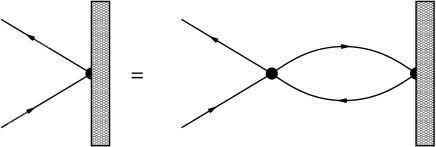
Figure 2: ${\cal R}$ matrix constraint.

Although, for an interacting integrable two-dimensional quantum field theory confined on a space segment of length $R$ equation (58) becomes exact only in the asymptotically large $R$ limit, it reveals that one of the main ingredients for the computation of the spectrum is, beside the exact bulk $S$ matrix a consistent reflection factor ${\cal R}(p)$. For massive integrable quantum field theories, the basic axiomatic constraints linking the boundary reflection factor ${\cal R}(p)$ to the two body $S$ matrix amplitude were discussed in [66, 67, 68]. The generalization of these results to a generic massless perturbed conformal field theories is a nice and partially open problem that certainly deserves further attention. However a full discussion of this topic would take us too far afield, and we shall postpone it to the future.

For the time being, we restrict the discussion to the $D=3$ case of [44], i.e. the theory of a single Bose field in two dimensions with left-right scattering amplitude

$$S_{1}(p,q)=e^{ipq/\sigma}~{}.$$ (59)

Partially based on $\text{TIM}\rightarrow\text{IM}$ boundary flows discussed in [69], we identify the relevant constraints to be

$${\cal R}(p){\cal R}^{*}(p)=1~{},$$ (60)

which coincides with unitary constraint for ${\cal R}(p)$, and

$${\cal R}(p){\cal R}(-p)=S_{1}(p,p)~{},$$ (61)

corresponding to the equality between the two scattering diagrams represented in Figure 2.

Given the $S$ matrix (59), the minimal solution to equations (60) and (61) is

$${\cal R}_{0}(p)=\sqrt{S_{1}(p,p)}=e^{ip^{2}/(2\sigma)}~{},$$ (62)

while multi parameter solutions have the general form

$${\cal R}(p)={\cal R}_{0}(p)\prod_{j=1}^{\infty}{\cal R}^{(2j-1)}_{\delta_{j}}(p)~{},$$ (63)

with

$${\cal R}^{(m)}_{\delta}(p)=e^{(ip)^{m}\delta}~{},~{}(\text{m~{}odd})~{}.$$ (64)

The functions (64) satisfy the simpler equation

$${\cal R}^{(m)}_{\delta}(p){\cal R}^{(m)}_{\delta}(-p)=1~{}.$$ (65)

The signs of the real parameters $\delta$’s appearing (63) are not constrained by (60) or (61). However, as it will clear from the results described in Section 6.2 below, for left-right symmetrical boundary conditions, the terms with the largest power $2j-1\geq 3$ of $p$ and $\delta_{j}\neq 0$ appearing in (63) should have a coefficient $\delta_{j}>0$, to ensure a proper convergence of the TBA integrals and consequently also the validity of the boundary TBA approach itself.

In conclusion, the number of possible reflection factors is infinite. Since, even for a simple conformal field theory such as the ${\cal M}_{3,4}$ model, the set of all possible boundary conditions corresponding to the superposition of Cardy’s boundary (pure) states [70] is infinite dimensional, such a proliferation of free parameter reflection factors is not totally surprising.

6 The boundary TBA

The relevant TBA equation for our simple system, obeying Bose type statistics and defined on a infinite strip of size $R$ and boundary conditions $(\alpha,\beta)$, is [71, 72]

$$\epsilon(p)=2Rp+\Lambda(p)+\frac{p}{\sigma}\int_{{\bar{\cal C}}}\frac{dq}{2\pi}L(q)~{},$$ (66)

with

$$L(q)=\text{ln}_{{\bar{\cal C}}}\left(1-e^{-\epsilon(q)}\right)~{},~{}~{}\Lambda(p)=\text{ln}\left({\cal R}_{\alpha}(-ip)/{\cal R}_{\beta}(ip)\right)~{},$$ (67)

and vacuum and excited state energies

$$E^{(\text{TBA})}_{n}(R)=\int_{{\bar{\cal C}}}\frac{dp}{2\pi}L(p)~{}.$$ (68)

6.1 Basic boundary conditions

Let us first consider the basic boundary conditions

$$\Lambda(p)=\text{ln}\left({\cal R}_{0}(-ip)/{\cal R}_{0}(ip)\right)=0~{},$$ (69)

the TBA equation reduces to

$$\epsilon(p)=2Rp+\frac{p}{\sigma}\int_{{\bar{\cal C}}}\frac{dq}{2\pi}L(q)~{}.$$ (70)

The same logical steps described in Section A can be repeated to find the following simple algebraic constraint

$$E^{(\text{TBA})}_{n}(R)=-\frac{\pi c({\bar{\cal C}})}{12(2R+E^{(\text{TBA})}_{n}(R)/\sigma)}~{},$$ (71)

with $c({\bar{\cal C}})=1-24n$, ($n\in{\mathbb{N}}$). Considering only the positive energy solutions, we have

$$E^{(\text{TBA})}_{n}(R)+\sigma R=\sqrt{\sigma^{2}R^{2}+2\pi\sigma\left(n-\frac{1}{24}\right)}~{}.$$ (72)

Equation (72) coincides with the NG open string spectrum (11) at $D=3$. To check the full consistency with the BA equation (58), let us consider the single particle excited state

$$\epsilon(p)=2Rp+\text{ln}S_{1}(p,-ip_{j})+\frac{p}{\sigma}\int_{0}^{\infty}\frac{dq}{2\pi}L(q)~{},$$ (73)

where $q=-ip_{j}$ is the branch point of $L(q)$ corresponding to $\epsilon(-ip_{j})=-i2\pi n_{j}$, ($n_{j}=1,2,\dots$). At large $R$, setting $\epsilon(ip_{j})=i2\pi n_{j}$ on the LHS of (73) and dropping the exponentially subdominant term on the RHS

$$i2\pi n_{j}\simeq i2Rp_{j}+\text{ln}S_{1}(ip_{j},-ip_{j})=i2Rp_{j}+\text{ln}S_{1}(p_{j},p_{j})~{},$$ (74)

or

$$e^{i2Rp_{j}}S_{1}(p_{j},p_{j})=e^{i2Rp_{j}}{\cal R}_{0}(p_{j}){\cal R}_{0}(p_{j})\simeq 1~{}.$$ (75)

The result (75) nicely fits equation (58).

6.2 More general boundary conditions

Let us now consider the case

$${\cal R}(p)={\cal R}_{0}(p){\cal R}_{\delta_{1}}^{(1)}(p)=e^{ip^{2}/2\sigma}e^{i\delta_{1}p}~{},~{}~{}$$ (76)

since

$$\Lambda(p)=\text{ln}\left({\cal R}(-ip)/{\cal R}(ip)\right)=2p\delta_{1}~{},$$ (77)

we see that these boundary conditions simply correspond to a shift $R\rightarrow R+\delta_{1}$, the resulting exact spectrum is

$$E^{(\text{TBA})}_{n}(R,\delta_{1})=E^{(\text{TBA})}_{n}(R+\delta_{1})~{}.$$ (78)

Note that this case corresponds to the $b_{1}$ term in the boundary action (5). This correction was first calculated at first order in $b_{1}$ in [9] using the $\zeta-$function regularization and in [27] using dimensional regularization. In the latter reference it was also noted that this boundary term corresponds to a shift in $R$ and that this rule actually extends to the next order in $b_{1}$. In our approach this “shift” property is valid at any order of $\delta_{1}$ and the precise relation between $\delta_{1}$ and $b_{1}$ is $\delta_{1}=-4b_{1}$.

Further, we know that Lorentz symmetry of the target space, as pointed out in (8), makes this term inconsistent, yet the TBA approach is perfectly consistent. This clearly shows that the quantum integrability does not imply Lorentz invariance on the target space, as anticipated in the Introduction.

Consider now the case

$${\cal R}(p)={\cal R}_{0}(p){\cal R}_{\delta_{2}}^{(3)}(p)=e^{ip^{2}/(2\sigma)}e^{-ip^{3}\delta_{2}}~{},~{}~{}\Lambda(p)=\text{ln}\left({\cal R}(-ip)/{\cal R}(ip)\right)=2p^{3}\delta_{2}~{}.$$ (79)

The corresponding TBA equations are

$$\epsilon(p)=2Rp+2p^{3}\delta_{2}+\frac{p}{\sigma}\int_{{\bar{\cal C}}}\frac{dq}{2\pi}L(q)~{}.$$ (80)

The solution to (80) is of the form

$$\epsilon(p)=2R\kappa p+2p^{3}\beta~{},$$ (81)

with

$$\kappa+\frac{p^{2}}{R}\beta=1+\frac{p^{2}}{R}\delta_{2}+\frac{1}{2R\sigma}\int_{{\bar{\cal C}}}\frac{dq}{2\pi}\text{ln}\left(1-e^{-2R\kappa q-2q^{3}\beta}\right)~{}.$$ (82)

Then it must be exactly $\beta=\delta_{2}$ and the TBA yields an exact equation for the energy in terms of $\kappa=\kappa(\sqrt{\sigma}R,\delta_{2}/R^{3})$

$$\kappa=1+\frac{1}{2R\sigma}\int_{{\bar{\cal C}}}\frac{dq}{2\pi}\text{ln}\left(1-e^{-2R\kappa q-2q^{3}\delta_{2}}\right)~{},$$ (83)

which can be easily solved numerically for $R>0$ and $\delta_{2}>0$. Yet, in the literature there are interesting, large $R$, asymptotic corrections to the NG formula which we can match very easily. In fact, we can expand in the form

$$\text{ln}\left(1-e^{-2R\kappa p-2p^{3}\delta_{2}}\right)=\text{ln}\left(1-e^{-2R\kappa p}\right)+\left(\frac{2p^{3}\delta_{2}}{e^{2\kappa pR}-1}\right)+\dots$$ (84)

obtaining, for $\delta_{2}/R^{3}$ small,

$$\kappa=1+\frac{1}{4\pi\sigma R}\left(-\frac{\text{Li}_{2}(1,{\bar{\cal C}})}{2R\kappa}+\frac{3\delta_{2}}{4R^{4}}\text{Li}_{4}(1,{\bar{\cal C}})\right)+\dots~{},$$ (85)

which has solution

$$\kappa=\frac{1}{2}\left(1+\sqrt{1-\frac{1}{2\pi\sigma R^{2}}\text{Li}_{2}(1,{\bar{\cal C}})}\right)+\frac{1}{4\pi\sigma R}\frac{3\delta_{2}}{4R^{4}}\text{Li}_{4}(1,{\bar{\cal C}})+\dots.$$ (86)

The continuous branch extension of $\text{Li}_{4}(1,{\bar{\cal C}})$ is given by  [53]

$$\text{Li}_{4}(1,{\bar{\cal C}})=\text{Li}_{4}(1)+\frac{8}{3}\pi^{4}\sum_{i}(n_{i})^{3}=\frac{\pi^{4}}{90}+\frac{8}{3}\pi^{4}\sum_{i}(n_{i})^{3}~{},~{}~{}n_{i}\in{\mathbb{N}}~{},$$ (87)

and the resulting modification to the Nambu-Goto spectrum turns out to be

$$E_{\{n_{i}\}}^{(\text{TBA})}(R,\delta_{2})=\sigma R(2\kappa-2)=E_{n}^{(\text{TBA})}(R)+\frac{\delta_{2}\pi^{3}}{4R^{4}}\left(\frac{1}{60}+4\sum_{i}(n_{i})^{3}\right)+\dots$$ (88)

with $n_{i}=0,1,\dots$, $n=\sum_{i}n_{i}$. Equation (88) matches the results displayed in the Table on page 9 of [43], provided we set $D=3$ and identify $\delta_{2}=-4b_{2}$.

Returning to the positivity issue, briefly mentioned at the end of Section 5, notice that the integral appearing in equation (80) is divergent for $\delta_{2}<0$. It is therefore important to check the sign of the latter coefficient obtained from numerical simulations.

The $n=0$ state of the spectrum (88) was compared with numerics in the case of the three dimensional $SU(2)$ lattice gauge theory in [46]: $({\sigma})^{3/2}b_{2}\simeq-0.015(6)(6)$. $b_{2}$ was also evaluated in [31] for a class of holographic confining gauge theories and also in this case, with Dirichlet’s boundary conditions, the $b_{2}$ coefficient is negative. Thus, in both cases, the TBA equation (80) should provide a qualitatively good description of the deviation of the Nambu-Goto spectrum (11), caused by the presence of $b_{2}$-perturbed boundaries, over a wide range of $1/\sigma R^{2}$ about the infrared fixed point.

Further, an high precision numerical simulation of the three dimensional Ising gauge model was reported very recently in [32]. The agreement with the theoretical prediction turned out to be very good allowing a precise estimate of the boundary parameter $b_{2}$. The numerical outcome, $({\sigma})^{3/2}b_{2}\simeq 0.032(2)$, leads now to a negative sign for $\delta_{2}$. We interpret this result as a clear signal of the presence of additional (infrared subleading) contributions associated to extra terms with higher powers of $p$ in the boundary factor $\Lambda(p)$ and/or in the TBA convolution kernel. We shall postpone a more complete discussion on this issue and a comparison between TBA and Monte Carlo results to the future.

7 Conclusions

In this paper we pointed out that the effective string theory describing the confining colour flux tube which joins a static quark-antiquark pair can be seen as a two-dimensional CFT of central charge $D-2$ perturbed by the composite field $T\bar{T}$ made with the energy momentum tensor $T$. This perturbation is quantum integrable and the spectrum can be calculated with the TBA, as first noted in [44]. We generalized this result to a large class of conformal models. In the case of periodic boundary conditions the energy levels $E_{(n,\bar{n})}(R)$ are labeled by two integers $n$ and $\bar{n}$ which depend on the monodromy of the dilogarithm in the complex plane of the momentum $p$. In a generic ADE system these energies can be parametrised in the form $E_{(n,\bar{n})}(R)=\sigma R+\mathcal{E}+\bar{\cal E}$, where the two quantities $\mathcal{E}$ and $\bar{\cal E}$ obey the following consistency conditions

$$\mathcal{E}=-\frac{\pi(\tilde{\text{c}}_{\text{IR}}-24n)}{12(R+\bar{\cal E}/\sigma)}~{},~{}~{}~{}\bar{\cal E}=-\frac{\pi(\tilde{\text{c}}_{\text{IR}}-24\bar{n})}{12(R+\mathcal{E}/\sigma)}\,,$$ (89)

where $\tilde{\text{c}}_{\text{IR}}$ is the effective central charge. The solution of these two algebraic equations is exactly the NG spectrum. We then discussed the degeneracy of these states which is growing exponentially for large $n$ and $\bar{n}$. Similar conclusions can be drawn for the open string case, where we wrote and solved the boundary TBA. We found that the reflection factor may depend on a set of arbitrary parameters which are associated to the coupling constants of the boundary string action. The deviation of the NG spectrum due to these terms can be easily calculated, at least at the first order in these coupling constants, and it turns out that the results coincide with those of the standard perturbative calculations. These results give a novel perspective on the TBA, and will hopefully lead to a new way to study the interquark potential by means of nonlinear integral equations, exact $S$ matrices and form-factors for correlation functions.

One of the most interesting open questions of the present approach is tied to the fact that the above equations for each pair $n,\bar{n}$ admit two solutions $\pm E_{(n,\bar{n})}(R)$. Thus this theory has an infinite set of negative energy levels. Even if the theory can be fermionized and we may assume that the sea of negative energy states is completely filled we did not succeed in evaluating the zero-point energy associated to it and its possible effect on the NG spectrum. One possible way out is to assume that at a given perturbative order in the $1/{\sigma R^{2}}$ expansion of the NG spectrum some other irrelevant operator starts to contribute. This is in particular what happens in the massless flow from the tricritical Ising model to the critical one, which was the starting point of our analysis.

As a final remark we notice that TBA equations –both with and without boundaries– have emerged in the context of ${\cal N}=4$ super Yang-Mills for the study of the quark-antiquark potential [73, 74] and gluon scattering amplitudes [75]. The latter quantities are equivalent to light-like polygonal Wilson loops and thus correspond to the area of minimal surfaces in $AdS_{5}$ in the classical string theory limit. Although there are some similarities between the current setup and those of [73, 74] and [75], there are also important differences in the underlying physics and the analytic properties of the corresponding TBA equations and we are currently unable to identify a precise link between the results of [38], further developed here, and these important preceding works on $AdS_{5}/CFT_{4}$.

Acknowledgments – This project was partially supported by INFN grants IS FI11, P14, PI11, the Italian MIUR-PRIN contract 2009KHZKRX-007 “Symmetries of the Universe and of the Fundamental Interactions”, the UniTo-SanPaolo research grant Nr TO-Call3-2012-0088 “Modern Applications of String Theory” (MAST), the ESF Network “Holographic methods for strongly coupled systems” (HoloGrav) (09-RNP-092 (PESC)) and MPNS–COST Action MP1210 “The String Theory Universe”.

Appendix A The ADE general case

The analysis described in Section 3 can be immediately generalised to any perturbed conformal field theory with known exact $S$ matrix description, as for example, the massive theories represented by the diagonal reflectionless ADE-related scattering models of [50, 56]. The TBA equations are

$$\epsilon_{i}(p)=Re_{i}(p)-\sum_{j=1}^{N}\int_{{\cal C}_{j}}\frac{dq}{2\pi}~{}\phi_{ij}(p,q)~{}L_{j}(q)~{},~{}~{}\bar{\epsilon}_{i}(p)=Re_{i}(p)-\sum_{j=1}^{N}\int_{{\bar{\cal C}}_{{}_{j}}}\frac{dq}{2\pi}~{}\phi_{ij}(p,q)~{}\bar{L}_{j}(q)~{},$$ (90)

where $e_{i}(p)=\sqrt{p^{2}+m_{i}^{2}}$ is the dispersion relation of the $i$-th particle and $N$ is the rank of the corresponding ADE algebra. The kernels are

$$\phi_{ij}(p)=-i\partial_{q}\ln S_{ij}(p,q)~{},$$ (91)

where $S_{ij}(p,q)$ are the $S$ matrix amplitudes of [57, 54, 58, 59] parametrised using the momenta $p$ and $q$ of the two particles involved in the scattering. In the ultraviolet regime $m_{i}R\rightarrow 0$ the TBA equations (90) show the decoupling of the pseudoenergies for right movers from the left mover ones

$$\epsilon_{i}(p)=R\hat{m}_{i}p-\sum_{j=1}^{N}\int_{{\cal C}_{j}}\frac{dq}{2\pi}~{}\phi_{ij}(p,q)~{}L_{j}(q)~{},~{}~{}\bar{\epsilon}_{i}(p)=R\hat{m}_{i}p-\sum_{j=1}^{N}\int_{{\bar{\cal C}}_{j}}\frac{dq}{2\pi}~{}\phi_{ij}(p,q)~{}\bar{L}_{j}(q)~{}.$$ (92)

In this limit, the energy can be found exactly [50]. The set of pure numbers $\hat{m}_{i}\equiv m_{i}/m_{1}$ and $i=1,\dots,N$ fix a relative scale among the particle species. They cannot be arbitrary numbers, but must be proportional to the components of the Perron-Frobeniuns eigenvector of the corresponding Cartan matrix. For the vacuum states all this has been analysed in [50, 56], furthermore here we wish to take into consideration excited states as well [61, 52, 60] by introducing complex contours ${\cal C}_{i}$ and ${\bar{\cal C}}_{i}$ for the continuous branch dilogarithm and fugacities $\{\lambda_{i}\}$ inside the statistical functions

$$L_{i}(p)=\text{ln}_{{\cal C}_{i}}(1+\lambda_{i}e^{-\epsilon_{i}(p)})~{},~{}~{}\bar{L}_{i}(p)=\text{ln}_{{\bar{\cal C}}_{i}}(1+\lambda_{i}e^{-\bar{\epsilon}_{i}(p)})\,\,.$$ (93)

The fugacities are all equal to unity for sectors related to the CFT identity operator, while they may assume different values for conformal families of other primary fields [62, 63, 52]. In the ultraviolet limit the energy is

$$E^{(\text{TBA})}_{(n,\bar{n})}(R)=\mathcal{E}+\bar{\cal E}~{},~{}~{}\mathcal{E}=-\frac{\pi}{12R}c({\cal C})~{},~{}~{}\bar{\cal E}=-\frac{\pi}{12R}c({\bar{\cal C}})~{},$$ (94)

where the constants

$$c({\cal C})=\frac{12}{\pi}\sum_{i=1}^{N}R\hat{m}_{i}\int_{{\cal C}_{i}}\frac{dp}{2\pi}L_{i}(p)~{},~{}~{}c({\bar{\cal C}})=\frac{12}{\pi}\sum_{i=1}^{N}R\hat{m}_{i}\int_{{\bar{\cal C}}_{i}}\frac{dp}{2\pi}\bar{L}_{i}(p)~{},$$ (95)

can be written in terms of the solutions to (90) and computed exactly using the dilogarithm trick [50, 64]. Besides, they are easily related to the conformal central charge $\text{c}_{\text{IR}}$ and the conformal weights $(h,\bar{h})$ of the primary fields

$$c({\cal C})=\tilde{\text{c}}_{\text{IR}}-24n~{},~{}~{}c({\bar{\cal C}})=\tilde{\text{c}}_{\text{IR}}-24\bar{n}~{},~{}~{}(n,\bar{n}\in{\mathbb{N}})~{},$$ (96)

and $\tilde{\text{c}}_{\text{IR}}=\text{c}_{\text{IR}}-24(h+\bar{h})$. The central charge and the conformal dimensions are those for the coset models [65]

$$\frac{\hat{{\cal G}}_{1}\times\hat{{\cal G}}_{1}}{\hat{{\cal G}}_{2}}~{},~{}~{}{\cal G}\in A_{N},D_{N},E_{N}~{}.$$ (97)

Let us now come to the announced generalisation of the analysis described in Section 3, and introduce the following variant of massless TBA equation for ADE systems

$$\epsilon_{i}(p)=Rp\hat{m}_{i}-p\frac{\hat{m}_{i}}{\sigma}\sum_{j=1}^{N}\hat{m}_{j}\int_{{\bar{\cal C}}_{j}}\frac{dq}{2\pi}\bar{L}_{j}(q)-\sum_{j=1}^{N}\int_{{\cal C}_{j}}\frac{dq}{2\pi}\phi_{ij}(p,q)~{}L_{j}(q)~{},$$ (98)

$$\bar{\epsilon}_{i}(p)=Rp\hat{m}_{i}-p\frac{\hat{m}_{i}}{\sigma}\sum_{j=1}^{N}\hat{m}_{j}\int_{{\cal C}_{j}}\frac{dq}{2\pi}L_{j}(q)-\sum_{j=1}^{N}\int_{{\bar{\cal C}}_{j}}\frac{dq}{2\pi}\phi_{ij}(p,q)~{}\bar{L}_{j}(q)~{}.$$ (99)

The elegant definition of effective length

$$r=R+\bar{\cal E}/\sigma~{},~{}~{}\bar{r}=R+\mathcal{E}/\sigma~{},$$ (100)

allows to recast equations (98) and (99) in the form (92), with

$$-r\mathcal{E}=\frac{\pi c({\cal C})}{12}=\sum_{i=1}^{N}r\hat{m}_{i}\int_{{\cal C}_{i}}\frac{dp}{2\pi}L_{i}(p)~{},~{}-\bar{r}\bar{\cal E}=\frac{\pi c({\bar{\cal C}})}{12}=\sum_{i=1}^{N}\bar{r}\hat{m}_{i}\int_{{\bar{\cal C}}_{i}}\frac{dp}{2\pi}\bar{L}_{i}(p)~{},$$ (101)

where, importantly, the $c({\cal C})$ and $c({\bar{\cal C}})$ coincide with those already introduced in (96) and computable via equations (92) and (95). Finally, the following self-consistent constraints must hold

$$\mathcal{E}=-\frac{\pi(\tilde{\text{c}}_{\text{IR}}-24n)}{12(R+\bar{\cal E}/\sigma)}~{},~{}~{}~{}\bar{\cal E}=-\frac{\pi(\tilde{\text{c}}_{\text{IR}}-24\bar{n})}{12(R+\mathcal{E}/\sigma)}\,.$$ (102)

The latter pair of algebraic equations for $\mathcal{E}$ and $\bar{\cal E}$ can be easily solved, giving

$$E_{(n,\bar{n})}(R)=\mathcal{E}+\bar{\cal E}+\sigma R=\pm\sqrt{\sigma^{2}R^{2}+4\pi\sigma\left(n+\bar{n}-\frac{\tilde{\text{c}}_{\text{IR}}}{12}\right)+\left(\frac{2\pi(n-\bar{n})}{R}\right)^{2}}\,\,.$$ (103)

In conclusion, we have shown that the spectrum of Nambu-Goto with $D-2=\tilde{\text{c}}_{\text{IR}}$ emerges from a wide class of TBA models. Actually, we can generalize this analysis to many other interesting models, including infinite families of perturbed CFT theories described by non-diagonal $S$ matrices and we suspect that (103) can be obtained for any CFT.

We end this Section with a further observation. It was noticed in [47] that for any two-dimensional quantum field theory the expectation values of the composite field $T\bar{T}$ admits an exact representation in terms of the expectation value of the energy-momentum tensor itself. Using the standard CFT convention and setting

$$T=-2\pi T_{zz}~{},~{}~{}\bar{T}=-2\pi T_{\bar{z}\bar{z}}~{},~{}~{}\Theta=2\pi T_{z\bar{z}}=2\pi T_{\bar{z}z}~{},$$ (104)

the result of [47], written using the double integer labeling introduced in the previous sections, on the cylinder is

$$\langle n,\bar{n}|T\bar{T}|n,\bar{n}\rangle=\langle n,\bar{n}|T|n,\bar{n}\rangle\langle n,\bar{n}|\bar{T}|n,\bar{n}\rangle-\langle n,\bar{n}|\Theta|n,\bar{n}\rangle^{2}~{}.$$ (105)

With the help of the following relations linking the expectation values of the energy-tensor components with the energy eigenvalues $E_{(n,\bar{n})}(R)$ and the total momentum of the state $P_{(n,\bar{n})}(R)=2\pi(n-\bar{n})/R$

$$\begin{split}\langle n,\bar{n}|T_{yy}|n,\bar{n}\rangle&=-\frac{1}{R}E_{(n,\bar{n})}(R)~{},~{}~{}\langle n,\bar{n}|T_{xx}|n,\bar{n}\rangle=-\partial_{R}E_{(n,\bar{n})}(R)~{},~{}~{}\\ \langle n,\bar{n}|T_{xy}|n,\bar{n}\rangle&=-\frac{i}{R}P_{(n,\bar{n})}(R)~{},\end{split}$$ (106)

we have [47]

$$\partial_{R}(E^{2}_{(n,\bar{n})}(R)-P^{2}_{(n,\bar{n})}(R))=-\frac{2R}{\pi^{2}}\langle n,\bar{n}|T\bar{T}|n,\bar{n}\rangle~{}.$$ (107)

Here, we would like to remark that inserting espression (103) for the energy levels in (107) leads to

$$\langle n,\bar{n}|T\bar{T}|n,\bar{n}\rangle=-\pi^{2}\sigma^{2},$$ (108)

exactly and independently from the particular state $(n,\bar{n})$ under consideration. Finally, using (108) in (105) gives

$${\langle n,\bar{n}|\Theta|n,\bar{n}\rangle}=\sqrt{\pi^{2}\sigma^{2}+\langle n,\bar{n}|T|n,\bar{n}\rangle\langle n,\bar{n}|\bar{T}|n,\bar{n}\rangle}~{}.$$ (109)

Since, $\Theta=0$ corresponds to a conformal invariant theory, the field $\Theta$ can be identified with the CFT perturbing operator, thus the exact result (109) should contain fundamental information on the further contributions needed in ( 16) and (33), or in an arbitray $T\bar{T}$ perturbed CFT, to build the full action associated to the Nambu-Goto like spectrum (103).

References

- [1] C. Itzykson, M.E. Peskin and J.-B Zuber, Roughening of Wilson’s surface, Phys. Lett. B95, 259 (1980); J. Kogut and J. Shigemitsu Crossover from weak to strong coupling in SU(N) lattice gauge theories, Phys. Rev. Lett. 45, 410 (1980); A. Hasenfratz, E. Hasenfratz and P. Hasenfratz, Generalized roughening transition and its effects on the string tension, Nucl. Phys. B180, 353 (1981).
- [2] J. M. Kosterlitz and D. J. Thouless, Ordering, metastability and phase transitions in two-dimensional systems, J. Phys. C6, 1181 (1973).
- [3] M. Luscher, K. Symanzik and P. Weisz, Anomalies of the free loop wave equation in the WKB Approximation, Nucl. Phys. B173, 365 (1980).
- [4] M. Luscher, Symmetry breaking aspects of the roughening transition in gauge theories, Nucl. Phys. B180, 317 (1981).
- [5] M. Hasenbusch and K. Pinn, Surface tension, surface stiffness, and surface width of the three-dimensional Ising model on a cubic lattice, Physica A192, 342 (1993), [arXiv:hep-lat/9209013 [hep-lat]].
- [6] M. Caselle, R. Fiore, F. Gliozzi, M. Hasenbusch and P. Provero, String effects in the Wilson loop: A high precision numerical test, Nucl. Phys. B486, 245 (1997), [arXiv:hep-lat/9609041 [hep-lat]].
- [7] K. J. Juge, J. Kuti and C. Morningstar, Fine structure of the QCD string spectrum, Phys. Rev. Lett. 90, 161601 (2003), [hep-lat/0207004].
- [8] B. Lucini and M. Teper, Confining strings in SU(N) gauge theories, Phys. Rev. D64, 105019 (2001), [arXiv:hep-lat/0107007 [hep-lat]].
- [9] M. Luscher and P. Weisz, Quark confinement and the bosonic string, JHEP 0207, 049 (2002), [arXiv:hep-lat/0207003 [hep-lat]].
- [10] M. Caselle, M. Pepe and A. Rago, Static quark potential and effective string corrections in the (2+1)-d SU(2) Yang-Mills theory, JHEP 10, 005 (2004), [arXiv:hep-lat/0406008].
- [11] M. Luscher, G. Munster and P. Weisz, How thick are chromoelectric flux tubes?, Nucl. Phys. B180, 1 (1981).
- [12] M. Caselle, F. Gliozzi, U. Magnea and S. Vinti, Width of long color flux tubes in lattice gauge systems, Nucl. Phys. B460, 397 (1996), [arXiv:hep-lat/9510019 [hep-lat]].
- [13] F. Gliozzi, M. Pepe and U.-J. Wiese, The width of the confining string in Yang-Mills theory, Phys. Rev. Lett. 104, 232001 (2010), [arXiv:1002.4888 [hep-lat]].
- [14] F. Gliozzi, M. Pepe and U.-J. Wiese, The width of the color flux tube at 2-Loop order, JHEP 1011, 053 (2010), [arXiv:1006.2252 [hep-lat]].
- [15] M. Caselle, R. Fiore, F. Gliozzi, M. Hasenbusch and K. Pinn, et al., Rough interfaces beyond the Gaussian approximation, Nucl. Phys. B432, 590 (1994), [hep-lat/9407002 [hep-lat]].
- [16] M. Caselle, M. Hasenbusch and M. Panero, Comparing the Nambu-Goto string with LGT results, JHEP 03, 026 (2005), [arXiv:hep-lat/0501027].
- [17] M. Caselle, M. Hasenbusch and M. Panero, High precision Monte Carlo simulations of interfaces in the three-dimensional ising model: A comparison with the Nambu-Goto effective string model, JHEP 0603, 084 (2006), [arXiv:hep-lat/0601023 [hep-lat]].
- [18] N. D. Hari Dass and P. Majumdar, String-like behaviour of 4-D SU(3) Yang-Mills flux tubes, JHEP 0610, 020 (2006), [hep-lat/0608024].
- [19] B. Bringoltz and M. Teper, Closed k-strings in SU(N) gauge theories : 2+1 dimensions, Phys. Lett. B663, 429 (2008), [arXiv:0802.1490 [hep-lat]].
- [20] A. Athenodorou, B. Bringoltz and M. Teper, The spectrum of closed loops of fundamental flux in D = 3+1 SU(N) gauge theories, PoS LAT, 223 (2009), [arXiv:0912.3238 [hep-lat]].
- [21] A. Athenodorou, B. Bringoltz and M. Teper, Closed flux tubes and their string description in D=2+1 SU(N) gauge theories, JHEP 05, 042 (2011), [arXiv:1103.5854 [hep-lat]].
- [22] A. Athenodorou, B. Bringoltz and M. Teper, Closed flux tubes and their string description in D=3+1 SU(N) gauge theories, JHEP 02, 030 (2011), [arXiv:1007.4720 [hep-lat]].
- [23] M. Caselle and M. Zago, A new approach to the study of effective string corrections in LGTs, Eur. Phys. J. C71, 1658 (2011), [arXiv:1012.1254 [hep-lat]].
- [24] M. Billo, M. Caselle and R. Pellegrini, New numerical results and novel effective string predictions for Wilson loops, JHEP 1201, 104 (2011), [arXiv:1107.4356 [hep-th]].
- [25] A. Mykkanen, The static quark potential from a multilevel algorithm for the improved gauge action, JHEP 1212, 069 (2012), [arXiv:1209.2372 [hep-lat]].
- [26] A. Athenodorou and M. Teper, Closed flux tubes in higher representations and their string description in D=2+1 SU(N) gauge theories, [arXiv:1303.5946 [hep-lat]].
- [27] M. Luscher and P. Weisz, String excitation energies in SU(N) gauge theories beyond the free-string approximation, JHEP 07, 014 (2004), [arXiv:hep-th/0406205].
- [28] O. Aharony and E. Karzbrun, On the effective action of confining strings, JHEP 06, 012 (2009), [arXiv:0903.1927 [hep-th]].
- [29] H. B. Meyer, Poincare invariance in effective string theories, JHEP 05, 066 (2006), [arXiv:hep-th/0602281].
- [30] O. Aharony, Z. Komargodski and A. Schwimmer, presented by O. Aharony at String 2009 conference, Rome.
- [31] O. Aharony and M. Field, On the effective theory of long open strings, JHEP 1101, 065 (2011), arXiv:1008.2636 [hep-th]].
- [32] M. Billo, M. Caselle, F. Gliozzi, M. Meineri and R. Pellegrini, The Lorentz-invariant boundary action of the confining string and its universal contribution to the inter-quark potential, JHEP 05, 130 (2012), [arXiv:1202.1984 [hep-th]].
- [33] F. Gliozzi, Dirac-Born-Infeld action from spontaneous breakdown of Lorentz symmetry in brane-world scenarios, Phys. Rev. D84, 027702 (2011), [arXiv:1103.5377 [hep-th]].
- [34] O. Aharony and M. Dodelson, Effective string theory and nonlinear Lorentz invariance, [arXiv:1111.5758 [hep-th]].
- [35] F. Gliozzi and M. Meineri, Lorentz completion of effective string (and p-brane) action, JHEP 1208, 056 (2012), [arXiv:1207.2912 [hep-th]].
- [36] M. Meineri, Lorentz completion of effective string action, in proceedings of Xth Quark confinement and the hadron spectrum, [arXiv:1301.3437 [hep-th]].
- [37] O. Aharony, M. Field and N. Klinghoffer, The effective string spectrum in the orthogonal gauge, JHEP 04, 048 (2012), [arXiv:1111.5757 [hep-th]].
- [38] S. Dubovsky, R. Flauger and V. Gorbenko, Effective string theory revisited, JHEP 1209, 044 (2012), [arXiv:1203.1054 [hep-th]].
- [39] O. Aharony and Z. Komargodski, The effective theory of long strings, [arXiv:1302.6257 [hep-th]].
- [40] J. F. Arvis, The exact Q anti-Q potential in Nambu string theory, Phys. Lett. B127, 106 (1983).
- [41] P. Goddard, J. Goldstone, C. Rebbi and C. B. Thorn, Quantum dynamics of a massless relativistic string, Nucl. Phys. B56, 109 (1973).
- [42] L. Mezincescu and P. K. Townsend, 3D strings and other anyonic things, Fortsch. Phys. 60, 1076 (2012), [arXiv:1111.3384 [hep-th]].
- [43] O. Aharony and N. Klinghoffer, Corrections to Nambu-Goto energy levels from the effective string action, JHEP 12, 058 (2010), [arXiv:1008.2648 [hep-th]].
- [44] S. Dubovsky, R. Flauger and V. Gorbenko, Solving the simplest theory of quantum gravity, JHEP 1209, 133 (2012), [arXiv:1205.6805 [hep-th]].
- [45] S. Dubovsky, R. Flauger and V. Gorbenko, Evidence for a new particle on the worldsheet of the QCD flux tube, [arXiv:1301.2325 [hep-th]].
- [46] B. B. Brandt, Probing boundary-corrections to Nambu-Goto open string energy levels in 3d SU(2) gauge theory, JHEP 02, 040 (2011), [arXiv:1010.3625 [hep-lat]].
- [47] A. B. Zamolodchikov, Expectation value of composite field in two-dimensional quantum field theory, [hep-th/0401146].
- [48] K. Dietz and T. Filk, On the renormalization of string functionals, Phys. Rev. d27, 2944 (1983).
- [49] A. B. Zamolodchikov, From tricritical Ising to critical Ising by thermodynamic Bethe Ansatz, Nucl. Phys. B358, 524 (1991).
- [50] A. B. Zamolodchikov, Thermodynamic Bethe Ansatz in relativistic models. Scaling three state Potts and Lee-Yang models, Nucl. Phys. B342, 695 (1990).
- [51] T. R. Klassen and E. Melzer, Spectral flow between conformal field theories in (1+1)-dimensions, Nucl. Phys. B370, 511 (1992).
- [52] P. Dorey and R. Tateo, Excited states by analytic continuation of TBA equations, Nucl. Phys. B482, 639 (1996), [hep-th/9607167].
- [53] L. Vepstas, An efficient algorithm for accelerating the convergence of oscillatory series, useful for computing polylogarithm and Hurwitz zeta functions, [arXiv:math/0702243].
- [54] H. W. Braden, E. Corrigan, P. E. Dorey and R. Sasaki, Affine Toda field theory and exact S matrices, Nucl. Phys. B338, 689 (1990).
- [55] M. Caselle, L. Castagnini, A. Feo, F. Gliozzi and M. Panero, Thermodynamics of SU(N) Yang-Mills theories in 2+1 dimensions I - The confining phase, JHEP 1106, 142 (2011), [arXiv:1105.0359 [hep-lat]].
- [56] T. R. Klassen and E. Melzer, The thermodynamics of purely elastic scattering theories and conformal perturbation theory, Nucl. Phys. B350, 635 (1991).
- [57] T. R. Klassen and E. Melzer, Purely elastic scattering theories and their ultraviolet limits, Nucl. Phys. B338, 485 (1990).
- [58] V. A. Fateev and A. B. Zamolodchikov, Conformal field theory and purely elastic S matrices, Int. J. Mod. Phys. A5, 1025 (1990).
- [59] P. Christe and G. Mussardo, Integrable systems away from criticality: The Toda field theory and S matrix of the tricritical Ising model, Nucl. Phys. B330, 465 (1990).
- [60] P. Dorey and R. Tateo, Excited states in some simple perturbed conformal field theories, Nucl. Phys. B515, 575 (1998), [hep-th/9706140].
- [61] V. V. Bazhanov, S. L. Lukyanov and A. B. Zamolodchikov, Integrable quantum field theories in finite volume: Excited state energies, Nucl. Phys. B489, 487 (1997), [hep-th/9607099].
- [62] M. J. Martins, Complex excitations in the thermodynamic Bethe ansatz approach, Phys. Rev. Lett. 67, 419 (1991).
- [63] P. Fendley, Excited state thermodynamics, Nucl. Phys. B374, 667 (1992), [hep-th/9109021].
- [64] A. Kuniba and T. Nakanishi, Spectra in conformal field theories from the Rogers dilogarithm, Mod. Phys. Lett. A7, 3487 (1992), [hep-th/9206034].
- [65] P. Goddard, A. Kent and D. I. Olive, Virasoro Algebras and Coset Space Models, Phys. Lett. B152, 88 (1985).
- [66] A. Fring and R. Koberle, Factorized scattering in the presence of reflecting boundaries, Nucl. Phys. B421, 159 (1994), [hep-th/9304141].
- [67] S. Ghoshal and A. B. Zamolodchikov, Boundary S matrix and boundary state in two-dimensional integrable quantum field theory, Int. J. Mod. Phys. A9, 3841 (1994), [Erratum-ibid. A9, 4353 (1994)], [hep-th/9306002].
- [68] P. Dorey, R. Tateo and G. Watts, Generalizations of the Coleman-Thun mechanism and boundary reflection factors, Phys. Lett. B448, 249 (1999),[hep-th/9810098].
- [69] P. Dorey, C. Rim and R. Tateo, Exact g-function flow between conformal field theories, Nucl. Phys. B834, 485 (2010), [arXiv:0911.4969 [hep-th]].
- [70] J. L. Cardy, Boundary conditions, fusion rules and the Verlinde formula, Nucl. Phys. B324, 581 (1989).
- [71] A. LeClair, G. Mussardo, H. Saleur and S. Skorik, Boundary energy and boundary states in integrable quantum field theories, Nucl. Phys. B453, 581 (1995), [hep-th/9503227].
- [72] P. Dorey, A. Pocklington, R. Tateo and G. Watts, TBA and TCSA with boundaries and excited states, Nucl. Phys. B525, 641 (1998), [hep-th/9712197].
- [73] N. Drukker, Integrable Wilson loops, [arXiv:1203.1617 [hep-th]].
- [74] D. Correa, J. Maldacena and A. Sever, The quark anti-quark potential and the cusp anomalous dimension from a TBA equation, JHEP 1208, 134 (2012) [arXiv:1203.1913 [hep-th]].
- [75] L. F. Alday, J. Maldacena, A. Sever and P. Vieira, Y-system for Scattering Amplitudes, J. Phys. A43, 485401 (2010) [arXiv:1002.2459 [hep-th]].