Computational investigation of plastic deformation
in face-centered cubic materials

Abstract

A mathematical model of plastic deformation in face-centered cubic (FCC) materials based on a balance model taking into account fundamental properties of deformation defects of a crystal lattice was developed. This model is based on a system of ordinary differential equations (ODE) accounting for various mechanisms of generation and annihilation of deformation defects for different external conditions. In-house developed software, SPFCC (Slip Plasticity of Face-Centered Cubic), was employed to solve the system of ordinary differential equations. The implemented code solves efficiently the stiff ODE system and provides a user-friendly interface for investigation of various features of plastic deformation in FCC materials.

Simulation of plastic deformation in the FCC metals was performed for the case of constant strain rate. The modelling results were validated by comparing experimental data and simulation results (stress-strain curves) and good agreement was obtained.

Computational Materials Science M.E. Semenov et al. 2011Published by Elsevier Ltd.

1 Introduction

The role and possibilities of mathematical modelling and computer simulation in the analysis of plastic deformation are of great importance. The mathematical modelling allows to reveal the role of various factors influencing processes of plastic deformation such as mechanisms responsible for strain hardening and evolution of deformation defects of crystalline materials [1, 2, 3, 4, 5]. Furthermore, the mathematical modelling is increasingly utilised for planning of experimental studies.

The mathematical modelling of plastic deformation in crystals is based on mathematical relationship taking into account fundamental properties of deformation defects of crystal lattice and represents a fundamental part of crystal plasticity models [4, 6, 7, 8, 9, 10]. The models usually consist of kinetic equation, which establishes a relationship between the current microstructure and the material’s mechanical response. This relationship,is written in general form as ordinary differential equations (ODE). Various models reported in literature [5, 6, 8, 11, 12, 13] differ from each other in way the set of deformation defects and the mechanisms of their generation and annihilation are considered.

Typically mathematical models of plastic deformation include the equations of deformation defects accounting for elementary processes and mechanisms of plasticity [4, 6, 7, 14]. Specifically, the choice of deformation defects, defining the regularities of plastic deformation and the mechanisms of their generation and annihilation and mutual transformation, determines the adequacy and possibilities of a mathematical model.

Crystallographic shear zone is selected as a basic structural element with which regard mechanisms of slip plasticity are considered in mathematical model of plastic deformation by slip [4, 10, 14, 15]. The description of the mechanisms of formation of shear zones formation is based on the fundamental physical and topological properties of defects responsible for plastic mass transfer. The fact that all parameters of the model either have physical or geometric interpretation or can be defined from physical considerations, or their values can be limited to a certain interval of may be specified, is a characteristic feature of the model and represent a significant advantage over phenomenological models.

Plastic deformation of slip primarily produces dislocations of various types and point defects. The processes of initiations of defects during formation of crystallographic shear zones are the mechanisms defining their generation.

Mathematical model of plastic deformation in FCC metals [16, 17] consists of the balance equations of shear-producing dislocations (their density is denoted as $\rho_{m}$), dislocations in vacancy ($\rho_{d}^{v}$) and interstitial ($\rho_{d}^{i}$) dipole configurations, interstitial atoms (concentration $c_{i}$), monovacancies ($c_{1v}$) and divacancies ($c_{2v}$), the equation defining strain rate, and the equation describing external effects to the deformed material. The specific ingredients of the model of deformation defects generation and annihilation are derived from the assumption that:

1. The defects generation processes occur during the formation of crystallographic shear zones and are related to the dynamic nature of their formation.

2. Annihilation processes have predominantly diffusion nature and occur in defect medium created by a set of defects generated by the slip in a large number of shear zones.

3. Deformation defect continuum is homogeneous continuum and contains the same number of defects, that the entire crystallographic shear zones together.

The mechanisms of deformation defects generation during the formation of crystallographic shear zone in monocrystals of FCC metals are reviewed in section 2, and the mechanisms of defects annihilation are presented in section 3. Section 4 summarises the system of differential equations of the model of plastic deformation in FCC metals. Section 5 is devoted to the description of SPFCC software, aimed to automatize the investigation of regularities of plastic deformation by slip with the use of a mathematical model. Section 6 gives an illustrative example showing possibilities of SPFCC software.

2 The intensity of deformation defects generation in the formation of crystallographic shear zone

The intensity of shear-producing dislocations generation. The intensity of the generation of shear-producing dislocations during the formation of crystallographic shear zone was obtained in [18] based on the ideas of Indenbom V.L., Orlov A.K., and Kuhlmann-Wilsdorf D. [1, 15, 19]. If we assume that the process of deformation occurs in identical shear zones, the intensity of the generation of shear-producing dislocations with deformation can be described as follows [18]:

$$G_{m}(\rho)=F/(bD_{r}),$$ (1)

where $D_{r}=(B_{r}\tau)/(Gb\rho_{m})$ is an average diameter of the shear zone, $b$ is the magnitude of the Burgers vector, parameter $F$ is determined by the geometry of the dislocation loops and their distribution in the shear zone [18], $B_{r}$ is the parameter determined by the probability of formation of extended dislocation barriers, $\tau$ is the applied stress, $G$ is the shear modulus. The description of the parameters and variables of the mathematical model is summirised in Tabl1 (see Appendix A).

Dislocations in dipole configurations are generated during the formation of crystallographic shear zone. The main cause for the occurrence of these dislocations is the presence of immobile dislocation jogs. When moving, the jogs leave a chain of point defects in case the height of the jogs is equal to one interatomic distance. In cases where the height of the jogs is more than one interatomic distance a dipole is formed. The dislocation loops emitted by the source broaden rapidly, due to decrease in nonlocal curvature. This leads to the generation of point defects with increasing intensity, and orientation close to screw, and their entrapment after short period of time.

$$G_{di}(\rho)=G_{dv}(\rho)=(6\gamma_{d}l_{d}(\rho)b)^{-1},$$ (2)

where $\gamma_{d}$ is the size parameter of the particles, $l_{d}(\rho)$ is the length of the screw dislocation run.

The intensity of generation of point defects. Non-conservative movement of dislocations with jog leads to the generation of such point deformation defects as interstitial atoms, vacancies and divacancies. The intensity of generation of point defects can be calculated as

$$G_{k}(\rho)=2q\tau_{dyn}/G,$$ (3)

where $k=\{i,1v,2v\}$, $\tau_{dyn}$ is excessive stress (the stress excess over the static resistance to dislocation motion), and parameter $q$ characterizing local concentration of stress during shear zone formation.

If the distribution of forest dislocations is assumed random, and the intensity of vacancies and interstitial atoms generation is considered identical, the relation for the rate of the vacancies and the interstitial atoms generation is as follows:

$$G_{i}(\rho)=G_{1v}(\rho)=q\tau_{dyn}/G.$$ (4)

Taking into account the fact that the activation energy of divacancies migration is lower than the activation energy of monovacancies migration, and that divacancies migrate from vacancies chain behind threshold on dislocations to crystal volume presumably faster, the following relations for the intensity of mono- and divacancies generation during the process of deformation were derived:

$$G_{1v}(\rho)=q\tau_{dyn}/(6G),$$ (5)

$$G_{2v}(\rho)=5q\tau_{dyn}/(6G).$$ (6)

3 Mathematical modelling of deformation defects annihilation processes

Dislocations annihilation. A number of different mechanisms of dislocations annihilation have been presented in the literature [4, 6, 7, 10, 16, 18]. The main mechanisms of dislocations annihilation are: a) climb of non-screw dislocations as a result of precipitation of point defects on extra planes of non-screw dislocations, and b) annihilation of screw dislocations during their cross-slip.

The following mechanisms are considered for annihilation of dipole dislocation configurations:

1. Decrease in the shoulder of vacancy dislocation dipoles until their annihilation with precipitation of interstitial atoms onto them.

2. Decrease in the shoulder of interstitial dislocation dipoles until their annihilation with precipitation of monovacancies and divacancies onto them.

3. Increase of the shoulder of vacancy dislocation dipoles until the loss of their stability with precipitation of monovacancies and divacancies onto them.

4. Increase of the shoulder of interstitial dislocation dipoles until the loss of their stability with precipitation of interstitial atoms onto them.

Shear-producing dislocations annihilation by climb. Annihilation processes of diffusive nature in a dislocation subsystem include both climb of non-screw dislocations, and their counter-movement in the slip planes. Dislocations annihilation by crystallographic slip can occur only in pairs of dislocation segments, which are located closely enough to one another and have opposite Burgers vectors. The distance between such dislocation segments is defined by critical radius of capture:

$$r_{a}=\frac{Gb}{4\pi\tau_{f}}\frac{2-\nu}{1-\nu},$$

where $\tau_{f}$ is friction stress, $\nu$ is Poisson’s ratio.

At high density of dislocations when the distance between dislocations is less than $r_{a}$, it can be assumed that the distance between dislocation segments able to annihilate is equal to $\rho_{m}^{-1/2}$. Assuming that dipoles are distributed uniformly along the length of the shoulder and the distance between the dipoles in interval $[0,\rho_{m}^{-1/2}]$, then the expression for the rate of the shear-forming dislocations annihilation as a result of precipitation of interstitial atoms onto them can be written as:

$$A_{m}(\rho,c_{k})=2b^{-1}\rho_{m}min(r_{a},\rho_{m}^{-1/2})\omega_{m}^{i}/A_{i}(\rho,c_{k}),$$ (7)

where $A_{i}(\rho,c_{k})=Q_{k}c_{k}/\dot{a}$ is the rate of point defects annihilation, $k=\{i,1v,2v\}$, $Q_{k}$ is the diffusion coefficient, $\dot{a}$ is the strain rate, $\omega_{m}^{i}$ is the fraction of interstitial atoms which left the glide plane on which they are stored.

Screw dislocations annihilation by cross-slip. We assume that the cross-slip of dislocations occurs only at temperatures above a certain temperature $T_{cs}$ and is athermal. In this case, almost all screw dislocations annihilate if they are stable under current applied stress $\tau$ and are trapped in dipole configurations in which the distance between dislocations of the opposite sign does not exceed the distance $r_{a}=Gb/(2\pi\tau_{f})$. According to this approach the annihilation of screw dislocations by cross-slip can be represented by the relation:

$$A_{m}^{cs}(\rho_{m})=FG\rho_{m}\omega_{s}P_{as}/(B\tau),$$ (8)

where $P_{as}$ is the probability of annihilation of screw dislocations, $\omega_{s}$ is a fraction of screw dislocations.

Dislocations annihilation in dipole configurations. The main mechanism of dislocation annihilation in dipole configuration is the trapping of interstitial atoms on the vacancy dipoles, which leads to a decrease of the shoulder of the vacancy dipoles, and precipitation of interstitial atoms on interstitial dipoles.

Dislocations annihilation in vacancy dipole configurations. Suppose that the maximum shoulder of the dipole, after which it loses its stability, is equal to the critical radius of the capture $r_{a}$. In this case the rate of the dislocations annihilation in vacancy dipole configurations can be determined as follows:

$$A_{dv}(\rho,c_{i})=2\omega_{i}^{dv}A_{i}(\rho,c_{i})/(br_{a}).$$ (9)

Here $\omega_{i}^{dv}$ is the fraction of interstitial atoms, which left to vacancy dipoles.

The density of dislocations forming vacancy dipoles during precipitation of vacancies onto them does not change significantly until the length of dipole shoulder becomes higher than $r_{a}$. In this instance, dipoles loose stability and their further behaviour become analogous to that of the shear-forming dislocations. The rate of change of the density of dislocations in vacancy dipole configurations with deformation caused by precipitation of vacancies can be described as follows:

$$R_{dv}(\rho,c_{1v})=2\omega_{1v}^{dv}A_{1v}(\rho,c_{1v})/(br_{a}),$$ (10)

where $\omega_{1v}^{dv}$ is the fraction of vacancies, which left to vacancy dipoles.

The rate of change of the dislocation density in vacancy dipoles configurations connected with precipitation of monovacancies onto them can be described analogically:

$$R_{dv}(\rho,c_{2v})=2\omega_{2v}^{dv}A_{2v}(\rho,c_{2v})/(br_{a}),$$ (11)

where $\omega_{2v}^{dv}$ is the fraction of divacancies, which left to vacancy dipoles.

Dislocations annihilation in interstitial dipole configurations. Taking into account the fact that precipitation of vacancies onto interstitial dislocation dipoles leads to the decrease of the shoulder of the interstitial dislocation dipoles, whereas precipitation of interstitial atoms leads to the increase in their shoulder, similar to the intensity of the annihilation of vacancy dipoles considered above Eq. (9), we can write down the following relations for the intensity of the annihilation of interstitial dipole configurations in case of precipitation of mono- and divacancies onto them respectively:

$$A_{di}(\rho,c_{1v})=2\omega_{1v}^{di}A_{1v}(\rho,c_{1v})/(br_{a}),$$ (12)

$$A_{di}(\rho,c_{2v})=2\omega_{2v}^{di}A_{2v}(\rho,c_{2v})/(br_{a}),$$ (13)

where $\omega_{1v}^{di}$, $\omega_{2v}^{di}$ are the fractions of mono- and divacancies respectively, which left to interstitial dipoles.

For the intensity of change of the dislocations density in interstitial dipole configurations, which is connected with precipitation of interstitial atoms onto them, the following relation is used:

$$R_{di}(\rho,c_{i})=2\omega_{i}^{di}A_{i}(\rho,c_{i})/(br_{a}),$$ (14)

where $\omega_{i}^{di}$ is a fraction of interstitial atoms, which left to interstitial dipoles.

Annihilation of deformation point defects. During the process of plastic deformation, concentration of point defects is reduced as a result of their spending for the sinks. Dislocations, crystal grain boundaries, and crystal surface can act as the sinks for point defects. In this work, the following sinks are considered in particular models of point deformation defects annihilation: 1) for interstitial atoms – non-screw dislocations, mono-, divacancies; 2) for monovacancies – non-screw dislocations, interstitial atoms, monovacancies; 3) for divacancies – non-screw dislocations, interstitial atoms. The rates of change of the deformation defects concentration can be expressed as follows:

$$A_{k}(\rho,c_{k})=Q_{k}c_{k}/\dot{a}.$$ (15)

It should be noted that, when two vacancies in their random movement meet, divacancies are formed, and when a divacancy meets an interstitial atom, or an interstitial atom meets a divacancy, a monovacancy is formed. Therefore, relations of deformation point defects accumulation take into account an additive to monovacancies and divacancies accumulation:

$$R_{1v}(c_{2v},c_{i})=(Q_{i}+Q_{2v})c_{i}c_{2v}/\dot{a},$$ (16)

$$R_{2v}(c_{1v})=Q_{1v}c_{1v}^{2}/\dot{a}.$$ (17)

The cases of point defects formed as a result of the meeting of two divacancies or a mono- and a divacancy were not considered in this work.

4 The system of differential equations of deformation defects balance

The presented models of deformation defects generation and annihilation described in sections 2–3 provide the basis for the creation of model of plastic deformation by slip. This model can be used to analyse the influence of various mechanisms and processes for FCC metals under various conditions of deformation.

The system of differential equations of the balance of deformation defects for FCC metals can be summarized as follows [4]:

$$\displaystyle\frac{dc_{1v}}{da} =\frac{q\tau_{dyn}}{6G}-\frac{(Q_{1v}c_{1v}-(Q_{i}+Q_{2v})c_{i}c_{2v})}{\dot{a}},$$ (18)

$$\frac{dc_{2v}}{da} =\frac{5q\tau_{dyn}}{6G}-\frac{(Q_{2v}c_{2v}-Q_{1v}c_{1v}^{2})}{\dot{a}},$$

$$\frac{dc_{i}}{da} =\frac{q\tau_{dyn}}{G}-\frac{Q_{i}c_{i}}{\dot{a}},$$

$$\frac{d\rho^{v}_{d}}{da} =\frac{1}{6\gamma_{d}l_{d}(\rho)b}-\frac{2(\omega_{i}^{dv}A_{i}(\rho,c_{i})+\omega_{1v}^{dv}A_{1v}(\rho,c_{1v})+\omega_{2v}^{dv}A_{2v}(\rho,c_{2v}))}{br_{a}},$$

$$\frac{d\rho^{i}_{d}}{da} =\frac{1}{6\gamma_{d}l_{d}(\rho)b}-\frac{2(\omega_{1v}^{di}A_{1v}(\rho,c_{1v})+\omega_{2v}^{di}A_{2v}(\rho,c_{2v})+\omega_{id}^{i}A_{i}(\rho,c_{i}))}{br_{a}},$$

$$\frac{d\rho_{m}}{da} =\frac{F}{bDr}-\frac{FG\rho_{m}\omega_{s}P_{as}}{B\tau}-\frac{2\rho_{m}min(r_{a},\rho_{m}^{-1/2})}{b}\sum_{k=\{i,1v,2v\}}\frac{\omega_{m}^{k}}{A_{k}(\rho,c_{k})}+$$

$$+\frac{2(\omega_{1v}^{dv}A_{1v}(\rho,c_{1v})+\omega_{2v}^{dv}A_{2v}(\rho,c_{2v})+\rho_{i}^{di}A_{i}(\rho,c_{i}))}{br_{a}}.$$

The last equation of the system (18) takes into account the relaxation contribution due to the rate of change of the dislocations density in dipole configurations for the intensity of shear-forming dislocations accumulation.

The equations establishing the relationship between strain rate the applied stress as well as the defect condition of the material are taken from [4, 18]. In this work the following equation for the strain rate of plastic deformation is selected [4]:

$$\dot{a}=a_{0}\exp\left(-\frac{0,2Gb^{3}-(\tau-\tau_{a})\lambda(\tau,\rho)b^{2}}{kT\rho^{1/2}}\right),$$ (19)

where $\tau_{a}$ is an athermal component of stress, $\lambda(\tau,\rho)$ is the function of stress and density of dislocations, $a_{0}$ is pre-exponential factor.

The system of equations (18) should be added by an equation (or equations), describing the influence causing deformation.

5 SPFCC software description

A computational tool, denoted SPFCC (Slip Plasticity of Face-Centered Cubic), has been developed. This software can assist researchers in application of the mathematical models for the computational investigation of plastic deformation in FCC materials. Although, a number of commercial tool addressing this problem are readily available, a user needs to be familiar with methods of solving ODE and requires programming language skills in order to consider a specific problem.

SPFCC software makes it possible to automatically form and calculate a full or reduced suite of defects of a mathematical model with little user intervention to set up the input values, run the calculations, plot stress strain curves, and export the results [18]. SPFCC enables direct simulations of strain hardening and evolution of deformation defects of crystalline materials.

Presently, the following types of effects can be considered: deformation with a constant strain rate $\dot{a}=const$, at constant stress $\tau=const$ and constant load $P=const$ in conditions of tension $\tau=\tau_{0}exp(a/k_{s})$ and compression $\tau=\tau_{0}exp(-a/k_{s})$, where $k_{s}$ is Sachs factor.

Fig. 1 shows main window of the software SPFCC. Simulation results (stress-strain curves) for different external conditions are obtained in less than one minute and posses a relative accuracy of the solution $10^{-3}$. Fig. 1 illustrates the time of simulation results for constant strain rate at different temperatures. It should be noted that the computational time for the case of constant stress (creep) increases and the results are obtained in ten minutes. All the simulations were performed on the Supermicro computing cluster based on Intel Xeon Processor 5570 (code named “Nehalem”, http://www.cluster.tpu.ru).

SPFCC software helps to analyse the processes of plastic deformation in FCC metals and dispersion-strengthened materials with a metal FCC matrix and noncoherent, undeformable particles of the second phase [4].

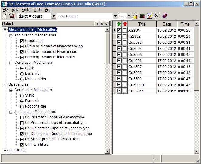
Figure 1: Main window of SPFCC software.

The user can either apply the full mathematical model, or create reduced models. The reduced model can take into account the deformation defects and mechanisms of their generation and annihilation specified by the user. At the beginning of a calculation, the starting suite of defects and initial value of parameters are selected from the database.

It should be noted that systems of ODE balance of deformation defects for various deformating effects and materials may differ in the number of equations and the mechanisms of defects generation and annihilation because user can to choose or disregard some mechanisms in the reduced models. In addition, the equations can be piecewise cross-linked type. This places some restriction on the choice and realization of a numerical method.

The system of differential equations of the model (18)–(19) is numerically stiff [17, 20]. This is mainly due to the fact that processes of generation and annihilation of deformation defects are significantly differ in terms of intensity. In addition value of variables are changing in the interval of integration by orders of magnitude.

In order to solve a stiff ODE system, the software package SPFCC employs the explicit linear multistep Adams method to obtain initial values and variable order multistep Gear method (in the form of backward differentiation formulas). The Gear method is stable at any integration stepsize, and therefore can choose an integration step guided only by considerations of accuracy, but not stability [20]. The original Gear method has been modified [17], due to some physical restrictions imposed on the variables of the equations system (for example, variables can not be negative). The analysis of the effectiveness of numerical algorithms for the case of plastic deformation of dispersion-strengthened materials with undeformable particles was given in publication [17].

The graphical user interface of the SPFCC software allows to select variables and mechanisms of the generation and annihilation of dislocations (Fig. 1). The user can chose values of the mathematical model parameters, initial conditions, and calculations accuracy in a dialogue mode. Furthermore, two material FCC metal or dispersion-strengthened material can be selected by the user.I n this case, the user will automatically be offered to choose the values of the parameters of material from the database software. It should be noted that the database is compiled using the results of theoretical and experimental studies available in literature. The user can accept the default values or set its own parameters values. If a user enters an incorrect values the SPFCC software will generate an error message and will prompt user to change value or to set the default values.

The user can perform a series of calculations with the help of SPFCC software. To run the calculation, the parameter of the mathematical model (stress or load, temperature, initial density of dislocations, etc.), needs to be chosen together with the interval and the step of this parameters.

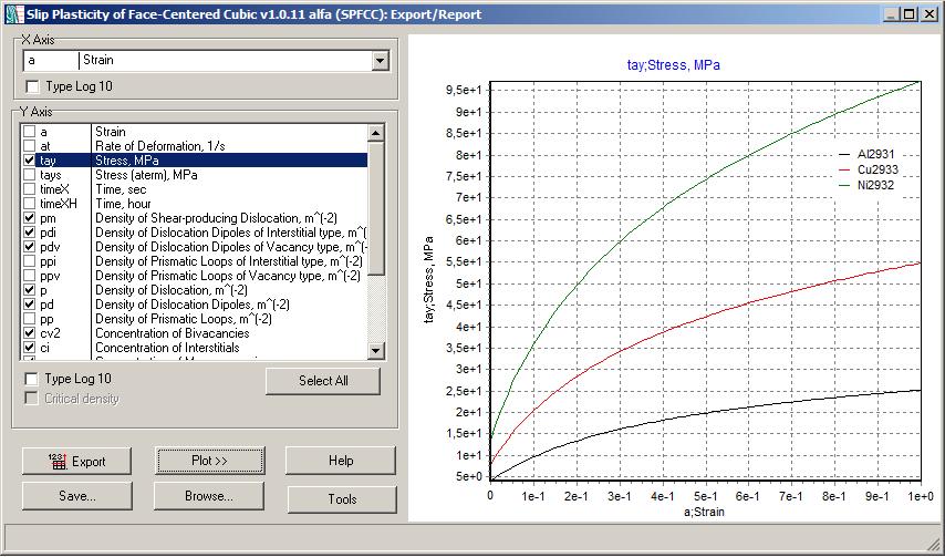
Figure 2: Dialogue window “Export/Report”.

In the process of the calculations it is possible to visualize intermediate results of modelling in real time, which allows to control the progress of calculations. The modelling results can be presented graphically. The user must tick the checkbox in the table “Modeling results” and click next on “Reports” button in the toolbar. Fig. 2 shows an example of the flow curves for various FCC metals (aluminum, copper, nickel) at the temperature $T=293K$.

Modelling results and the values of the model parameters used are saved in a local database automatically. Information regarding the progress of numerical solution of the task is also recorded in the database. This information allows to generate recommendations for further computer experiments.

The SPFCC software provides possibility to compare modelling results for various applied effects in tables and graphical form. According to modelling results, dependencies between any variables as well as temperature and strain rate dependency can be represented graphically.

6 Illustrative example

As an example of the model described above we show modelling results for the case of constant strain rate and its comparison with experimentally measured data. In case of the deformation of crystal with a constant strain rate, the equation of applied influence has the following form: $\dot{a}=const$. This is a transcendental equation, which allows to find the stress at any given time of the deformation.

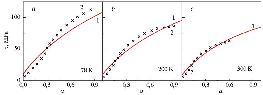
Figure 3: Flow stress for copper monocrystal: 1 – model data (solid line); 2 – experimental data (cross) [21]. The numbers near curves are the deformation temperature given in Kelvin degrees. The strain rate is $10^{-4}s^{-1}$.

Using the above-mentioned equations of deformation defects balance (18) and the equation defining strain rate (19), calculations were performed for FCC metals with the values typical for copper: $b=2.5\cdot 10^{10}m$, $\nu_{D}=10^{13}s^{-1}$, $\alpha=0.5$, $\tau_{f}=1MPa$, $\nu=1/3$, $k=1.38\cdot 10^{-23}J/K$, $\omega_{s}=0.3$. The initial density of shear-forming dislocations were chosen to be $10^{12}~{}m^{-2}$, and the initial density of dislocations in vacancy and interstitial dipole configurations and the concentration of interstitial atoms, vacancies, and divacancies were chosen to be zero. Fig. 3 shows strain hardening curves for copper monocrystal at various temperatures (solid lines) in comparison with experimental data [21]. A good agreement between experimental data and simulated curves is obtained.

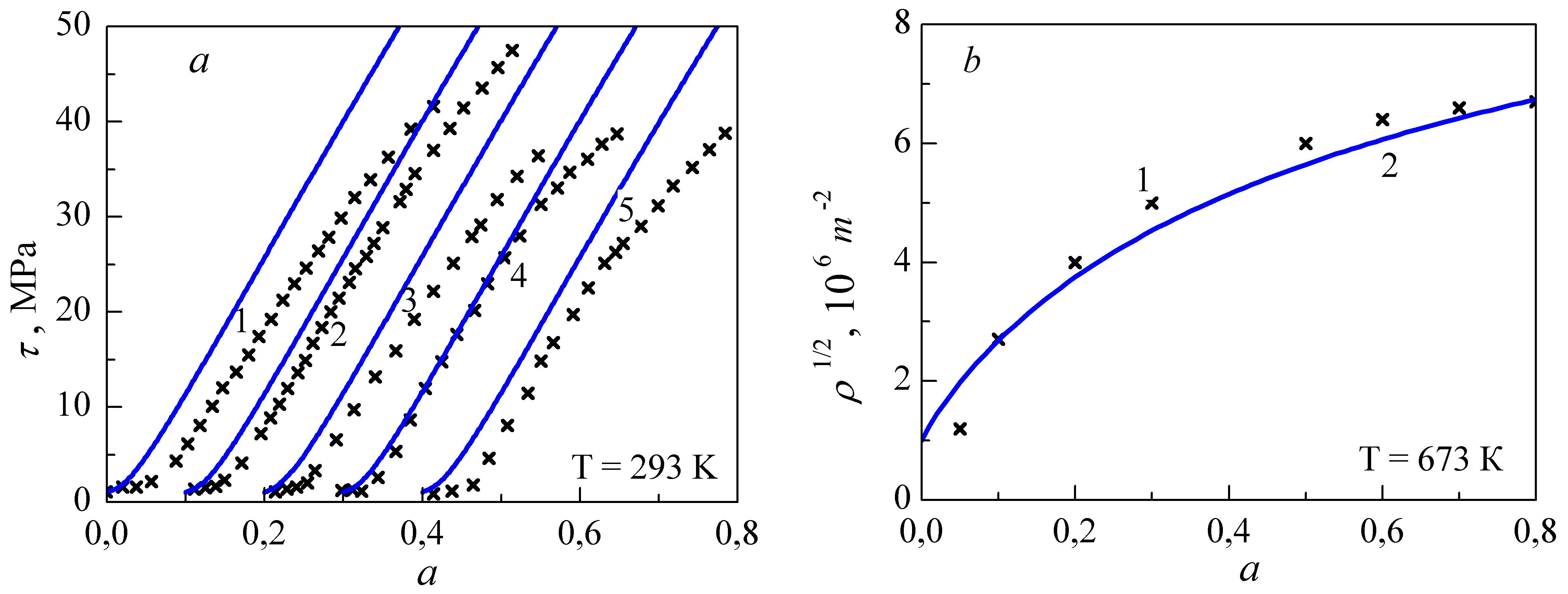
Figure 4: Flow stress for copper monocrystal: model data (solid line) and experimental data (cross) [22]. The numbers near curves are the strain rate given in $s^{-1}$: 1 – $1.27\cdot 10^{-2}$, 2 – $4.18\cdot 10^{-3}$, 3 – $4.34\cdot 10^{-4}$, 4 – $4.09\cdot 10^{-5}$, 5 – $4.46\cdot 10^{-6}$; (b). The square root of the dislocation density plotted versus the shear strain for copper monocrystal: 1 – experimental data [23], 2 – model data. The initial dislocation density is $10^{12}m^{-2}$ and the strain rate is $10^{-4}s^{-1}$.

Fig. 4a shows strain hardening curves for copper monocrystal at various strain rate (solid lines) in in comparison with experimental data [22]. Fig. 4b shows the square root of the dislocation density plotted versus the shear strain for copper monocrystal (solid line) in comparison with experimental data [23].

7 Conclusion

In this work a mathematical model of plastic deformation in FCC metals was presented. Various features of plastic deformation by slip under various loading conditions can be described within this model. The model was implemented in-house software SPFCC (Slip Plasticity of Face-Centered Cubic). It provides graphic user interface and supports a study of plastic deformation of FCC metals.

The “Slip Plasticity of Face-Centered Cubic” software creates a comfortable and friendly environment for computational experiments while modelling plastic deformation processes in both FCC-metals and the dispersion-strengthened materials under various loading conditions. The proposed modelling technic automates many user actions, allowing to explore a variety of factors influencing plastic deformation of FCC metals and dispersion-strengthened materials. The results of the calculation are stored in the database of the software and are available for future reference.The software also includes a number of tools for collaboration within the scientific community. Tabular representation of the results of the calculations is designed to export data to third-party software for further post-processing.

It should be noted that only the flow stress curves of copper with constant strain rate were considered in this work as an example. It was verified that the proposed mathematical model describes the plasticity of the FCC metals at various temperatures and strain rates accurately, and the results of computer simulation are in a good agreement with the experimental data. This computational investigation provides a fundamental understanding of the processes of intensity generation and annihilation of deformation defects of the centered cubic metals for constant strain rate. It’s also demonstrates the influence of the typical parameters values of FCC metals on the plastic deformation features.

8 Acknowledgements

This work was supported by the MSE Program “Nauka”, contract No. 1.604.2011. We thank Dr Andrey Molotnikov (Monash University, Australia) for critical reading and editorial suggestions for the manuscript.

Table 1: Description of Mathematical Model Variables and Parameters

Parameter	Description
$\rho$	total dislocation density
$\rho_{d}^{i}$	density of dislocation in the dipole configurations of the interstitial type
$\rho_{d}^{v}$	density of dislocation in the dipole configurations of the vacancy type
$\rho_{d}$	$=\rho_{d}^{v}+\rho_{d}^{i}$, density of dislocations in dipole configurations
$\rho_{m}$	density of shear-forming dislocations
$c_{1v}$	concentrations of monovacancies
$c_{2v}$	concentrations of divacancies
$c_{i}$	concentrations of interstitial atoms
$a$	shear strain
$\dot{a}$	strain rate
$B$	parameter, which is determined by the probability of dislocation barriers limiting the shear zone
$F$	parameter, which is determined by the shape of dislocation loops and their distribution in the slip zone
$q$	parameter that determines the intensity of point defects generation
$T$	temperature
$\alpha$	parameter of dislocations interaction
$b$	Burgers vector
$D$	diameter of the slip zone
$G$	shear modulus
$k$	Boltzmann constant
$\nu$	Poisson coefficient
$\omega_{s}$	fraction of screw dislocations
$P_{as}$	probability of annihilation of screw dislocations
$Q_{k}$	diffusion coefficient of point defects of the $k$th type $k=\{i,1v,2v\}$
$r_{a}$	critical capture radius
$\tau$	flow stress
$\tau_{dyn}$	stress excess over the static resistance to dislocation motion
$\tau_{f}$	friction stress
$\tau_{a}$	athermic component of the resistance to the dislocation gliding

References

- [1] D. Kuhlmann-Wilsdorf, Transact. Metall. Soc. AIME. 224 (1962) 1047–1061.
- [2] D.L. Preston, D.L. Tonks, D.C. Wallace, J. of App. Phys. 93 (2003) 211–220.
- [3] U. Kocks and H. Mecking, Prog. in Mater. Sci. 48 (2003) 171–273.
- [4] S.N. Kolupaeva, T.A. Kovalevskaya, O.I. Daneyko, M.E. Semenov, N.A. Kulaeva, Bull. Russian Acad. Sci.: Phys. 74 (2010) 1527–1531.
- [5] H.F. Zhan, Y.T. Gu, C. Yan, X.Q. Feng, P.K.D.V. Yarlagadda, Comput. Mater. Sci. 50 (2011) 3425–3430.
- [6] R. Lagneborg, Intern. Metals. Rev. 17 (1972) 130–146.
- [7] V. Essmann, H. Mughrabi, Phil. Mag. (a) 40 (1979) 731–756.
- [8] M. Mecking, U.F. Kocks, Acta Metal. 29 (1981) 1865–1875.
- [9] Y. Estrin, L.S. Toth, A. Molinari, Y. Brechet, Acta Mater. 46 (1998) 5509–5522.
- [10] L.E. Popov, S.N. Kolupaeva, N.A. Vihor, Comput. Mater. Sci. 19 (2000) 158–165.
- [11] F.J. Zerilli, R.W. Armstrong, J. of App. Phys. 5 (1987) 1816–1825.
- [12] G.Z. Voyiadjis, A.H. Almasri, Mechanics of Materials, 40 (2008) 549–563.
- [13] N.Q. Chinh, T. Csana di, J. Gubicza, T.G. Langdon, Acta Materialia 58 (2010) 5015 -5021.
- [14] L.E. Popov, S.N. Kolupaeva, N.A. Vihor, S.I. Puspescheva, Comput. Mater. Sci. 19 (2000) 267–274.
- [15] A.K. Orlov, Kinetics of dislocations, in: Theory of crystals defects, Publishing House of the Czechoslovak Acad. Sci., Prague, 1966, pp. 317–338.
- [16] S.N. Kolupaeva, S.I. Puspesheva, M.E. Semenov, Proc. book of 11-th Inter. Conf. on Fracture. Turin (Italy) (2005) 847.
- [17] M.E. Semenov, S.N. Kolupaeva, Tomsk Polytechnic University Bull. 317 (2010) 16–22.
- [18] L.E. Popov, V.S. Kobytev, T.A. Kovalevskaya, Izv. Vyssh. Uchebn. Zaved. Fizika, 6 (1982) 56–82.
- [19] V.L. Indenbom, Theory of dislocations – present state and future, in: Theory of crystals defects, Publishing House of the Czechoslovak Acad. Sci., Prague, 1966, pp. 2–16.
- [20] C.W. Gear, Numerical Initial Value Problem in Ordinary Differential Equations. First ed., Prentice-Hall Inc., 1971.
- [21] A. Seeger, J. Diehl, S. Mader, H. Rebstock, Phil. mag. 15 (1957) 323–350.
- [22] Z. Basinski, S. Basinski, Phil. Mag. (1964) 51- 80.
- [23] L.E. Popov, V.S. Kobytev, T.A. Kovalevskaya, Plastic deformation of allows. Moscow, 1984.