A Contraction Analysis of the Convergence of Risk-Sensitive Filters

Abstract

A contraction analysis of risk-sensitive Riccati equations is proposed. When the state-space model is reachable and observable, a block-update implementation of the risk-sensitive filter is used to show that the $N$-fold composition of the Riccati map is strictly contractive with respect to the Riemannian metric of positive definite matrices, when $N$ is larger than the number of states. The range of values of the risk-sensitivity parameter for which the map remains contractive can be estimated a priori. It is also found that a second condition must be imposed on the risk-sensitivity parameter and on the initial error variance to ensure that the solution of the risk-sensitive Riccati equation remains positive definite at all times. The two conditions obtained can be viewed as extending to the multivariable case an earlier analysis of Whittle for the scalar case.

1 Introduction

Starting with Kalman and Bucy’s paper [14], the convergence of the Kalman filter has been examined in detail, and it soon became clear that if the state-space model is stabilizable and detectable, the filter is asymptotically stable and the error covariance converges to the unique non-negative definite solution of a matching algebraic Riccati equation. However the classical Kalman filter convergence analysis [1, 13] is rather intricate and involves several steps, including first showing that the error covariance is upper bounded, next proving that with a zero initial value, it is monotone increasing, so it has a limit, and then establishing that the corresponding filter is stable and that the limit is the same for all initial covariances. In 1993, Bougerol [5] proposed a more direct convergence proof based on establishing that the discrete-time Riccati iteration is a contraction for the Riemmanian metric associated to the cone of positive definite matrices. Although this result attracted initially little notice in the systems and control community, this approach was adopted by several researchers [16, 17, 18, 20] to study the convergence of a number of nonlinear matrix iterations. We will use this viewpoint here to analyze the convergence of risk-sensitive estimation filters. Unlike the Kalman filter which minimizes the mean square estimation error, risk-sensitive filters [21, 23] minimize the expected value of an exponential of quadratic error index, which ensures a higher degree of robustness [10, 7] against modelling errors. Unfortunately, in spite of extensive studies on risk-sensitive and related $H^{\infty}$ filters, results concerning their convergence remain fragmentary [23, Chap. 9], [10, Sec. 14.6], [3]. In particular, one question that remains unresolved is whether there exists an a-priori upper bound on the risk-sensitivity parameter ensuring the convergence of the solution of the risk-sensitivite Riccati equation to a positive definite solution associated to a stable filter.

The contraction anaysis presented in this paper relies on a block implementation of Kalman (risk-neutral) and risk-sensitive filters. When the system is reachable and observable and the block length $N$ exceeds the number of states, it is shown that in the risk-neutral case, the Riccati equation corresponding to the block filter is strictly contractive, which allows us to conclude that the Riccati equation of Kalman filtering has a unique positive definite fixed point. This analysis is equivalent to the derivation of [5] which relied on showing that the $N$-fold composition of the Hamiltonian map associated to the risk-neutral Riccati operator is strictly contractive. However, it has the advantage that it can be extended easily to the risk-sensitive case by using the Krein-space formulation of risk-sensitive and $H^{\infty}$ filtering developed in [8, 9]. With this approach, it is is shown that the $N$-block risk-sensitive Riccati equation remains strictly contractive as long as a corresponding observability Gramian is positive definite. This Gramian is shown to be a monotone decreasing function of the risk-sensitivity parameter $\theta$ with respect to the partial order of non-negative definite matrices. Accordingly, it is possible to identify a priori a range $[0,\tau_{N})$ of values of the risk-sensitivity parameter $\theta$ for which the block Riccati equation is strictly contractive. This result is used to show that the risk-sensitive Riccati equation has a unique positive definite fixed-point, but because the image of the cone ${\cal P}$ of positive definite matrices under the risk-sensitive Riccati map is not entirely contained in ${\cal P}$ a second condition must be placed on $\theta$ and the initial variance $P_{0}$ of the filter to ensure that the evolution of the risk-sensitive Riccati equation stays in ${\cal P}$. The two conditions obtained can be viewed as extensions to the multivariable case of those presented in [23, Chap. 9] for scalar risk-sensitive Riccati equations.

The paper is organized as follows. The properties of the Riemann distance for positive definite matrices and of contraction mappings are reviewed in Section 2. The block-update filtering interpretation of the $N$-fold Riccati equation of Kalman filtering is described in Section 3 and is extended to the risk-sensitive case in Section 4. This formulation is used to estimate the range of values of the risk-sensitivity parameter for which the risk-sensitive Riccati equation is contractive. A second condition on the risk-sensitivity parameter and initial condition ensuring that the solution of the Riccati equation remains positive is obtained in Section 5. An illustrative example is studied in Section 6 and conclusions as well as a possible extension are presented in Section 7.

2 Riemann distance and contraction mappings

Let ${\cal P}$ denote the cone of positive definite symmetric matrices of dimension $n$, and let $\bar{\cal P}$ denote the cone of non-negative definite matrices forming the closure of ${\cal P}$. If $P$ is an element of ${\cal P}$ with eigendecomposition

$$P=U\Lambda U^{T}$$ (1)

where $U$ is an orthogonal matrix formed by normalized eigenvectors of $P$ and $\Lambda=\mbox{diag}\,\{\lambda_{1},\ldots,\lambda_{n}\}$ is the diagonal eigenvalue matrix of $P$, the symmetric positive square-root of $P$ is defined as

$$P^{1/2}=U\Lambda^{1/2}U^{T}$$

where $\Lambda^{1/2}$ is diagonal, with entries $\lambda_{i}^{1/2}$ for $1\leq i\leq n$. Similarly, the logarithm of $P$ is the symmetric, not necessarily positive definite, matrix specified by

$$\log(P)=U\log(\Lambda)U^{T}\>,$$

where $\log(\Lambda)$ is diagonal with entries $\log(\lambda_{i})$ for $1\leq i\leq n$. Let $P$ and $Q$ be two positive definite matrices of ${\cal P}$. Then $P^{-1}Q$ is similar to $P^{-1/2}QP^{-1/2}$, so they have the same eigenvalues, and $P^{-1/2}QP^{-1/2}$ is positive definite. Let $s_{1}\geq s_{2}\geq\ldots\geq s_{n}>0$ denote the eigenvalues of $P^{-1}Q$ sorted in decreasing order. The Riemann distance between $P$ and $Q$ is defined as

$$d(P,Q)=||\log(P^{-1/2}QP^{-1/2})||=\Big{(}\sum_{i=1}^{n}(\log(s_{i}))^{2}\Big{)}^{1/2}\>,$$ (2)

where $||.||$ denotes the matrix Frobenius norm. In addition to having all the traditional properties of a distance, $d$ has the feature that it is invariant under matrix inversion and congruence transformations. Specifically, if $M$ denotes an arbitrary real invertible matrix of dimension $n$,

$$d(P,Q)=d(P^{-1},Q^{-1})=d(MPM^{T},MQM^{T})\>.$$ (3)

Furthermore, it was also shown by Bougerol [5] that the translation of ${\cal P}$ by a non-negative definite symmetric matrix $S$ is a non-expansive map. Specifically,

$$d(P+S,Q+S)\leq\frac{\alpha}{\alpha+\beta}d(P,Q)$$ (4)

where $\alpha=\max(\lambda_{1}(P),\lambda_{1}(Q))$ and $\beta=\lambda_{n}(S)$. In these definitions, it is assumed that the eigenvalues of $P$, $Q$ and $S$ are sorted in decreasing order, so that $\lambda_{1}(P)$ is the largest eigenvalue of $P$, i.e., its spectral norm, and $\lambda_{n}(S)$ is the smallest eigenvalue of $S$.

Recall that if $f(\cdot)$ is an arbitrary mapping of ${\cal P}$, $f$ is non-expansive if

$$d(f(P),f(Q))\leq d(P,Q)\>,$$

and strictly contractive if

$$d(f(P),f(Q))\leq cd(P,Q)$$

with $0\leq c<1$. The least contraction coefficient or Lipschitz constant of a non-expansive mapping $f$ is defined as

$$c(f)=\sup_{P,Q\in{\cal P},P\neq Q}\frac{d(f(P),f(Q)}{d(P,Q)}\>.$$ (5)

Clearly, if $f$ and $g$ denote two non-expansive mappings, the contraction coefficient $c(f\circ g)$ of the composition of $f$ and $g$ satisfies $c(f\circ g)\leq c(f)c(g)$, so if at least one of the two maps is strictly contractive, the composition is also strictly contractive. From inequality (4), we deduce that if $\tau_{S}(P)=P+S$ denotes the translation by a positive definite matrix $S$, $\tau_{S}$ is non-expansive, but the bound (4) does not allow us to conclude that $c(\tau_{S})<1$, since when the largest eigenvalue of either $P$ or $Q$ goes to infinity, the constant $\alpha/(\alpha+\beta)$ tends to one.

The key result that will be used in this paper is that if $f$ is a strict contraction of ${\cal P}$ for the distance $d$, by the Banach fixed point theorem [2, p. 244], there exists a unique fixed point $P$ of $f$ in $\bar{\cal P}$ satisfying $P=f(P)$. Furthermore this fixed point can be evaluated by performing the iteration $P_{n+1}=f(P_{n})$ starting from any initial point $P_{0}$ of ${\cal P}$. Also if the $N$-fold composition $f^{N}$ of a non-expansive map $f$ is strictly contractive, then $f$ has a unique fixed point. We will consider in particular the Riccati-type map over ${\cal P}$ defined by

$$f(P)=M[P^{-1}+\Omega]^{-1}M^{T}+W$$ (6)

where $P$, $\Omega$ and $W$ are symmetric real positive definite matrices and $M$ is a square real, but not necessarily invertible, matrix. For this mapping the following result was established in [18, Th. 4.4].

Lemma 1.

$f$ is a strict contraction with

$$c(f)\leq\frac{\lambda_{1}(M\Omega^{-1}M^{T})}{\lambda_{n}(W)+\lambda_{1}(M\Omega^{-1}M^{T})}\>,$$ (7)

where we use again the convention that the eigenvalues of positive definite matrices are sorted in decreasing order.

Note that although the results presented in this paper use the Riemann distance over ${\cal P}$, other metrics such as the Thompson metric

$$d_{T}(P,Q)=\max(\lambda_{1}(\log(P^{-1/2}QP^{-1/2})),\lambda_{1}(\log(Q^{-1/2}PQ^{-1/2})))\>.$$ (8)

have similar properties [4, 11], and the Thompson metric is in fact often used to analyze the convergence of nonlinear matrix iterations [17, 20].

3 Block update filter

Consider a Gauss-Markov state space model

$$x_{t+1}=Ax_{t}+Bu_{t}$$ (9)

$$y_{t}=Cx_{t}+v_{t}\>,$$ (10)

where the state $x_{t}\in\mathbb{R}^{n}$, the process noise $u_{t}\in\mathbb{R}^{m}$ and the observation noise $v_{t}\in\mathbb{R}^{p}$. The noises $u_{t}$ and $v_{t}$ are assumed to be independent zero-mean WGN processes with normalized covariance matrices, so

$$E\Big{[}\left[\begin{array}[]{c}u_{t}\\ v_{t}\end{array}\right]\left[\begin{array}[]{cc}u_{s}^{T}&v_{s}^{T}\end{array}\right]\Big{]}=\left[\begin{array}[]{cc}I_{m}&0\\ 0&I_{p}\end{array}\right]\delta_{t-s}\>,$$

where

$$\delta_{t}=\left\{\begin{array}[]{cc}1&t=0\\ 0&t\neq 0\end{array}\right.$$

denotes the Kronecker delta function. The initial state vector $x_{0}$ is assumed independent of noises $u_{t}$ and $v_{t}$ and ${\cal N}(\hat{x}_{0},P_{0})$ distributed. Since we are interested in the asymptotic behavior of Kalman and risk-sensitive filters, the matrices $A$, $B$, and $C$ specifying the state-space model are assumed to be constant. Then if ${\cal Y}_{t-1}$ denotes the sigma field generated by observations $y(s)$ for $0\leq s\leq t-1$, the least-squares estimate $\hat{x}_{t}=E[x_{t}|{\cal Y}_{t-1}]$ depends linearly on the observations and can be evaluated recursively by the predicted form of the Kalman filter specified by

$$\hat{x}_{t+1}=A\hat{x}_{t}+K_{t}\nu_{t}\>,$$ (11)

where the innovations process

$$\nu_{t}\stackrel{{\scriptstyle\triangle}}{{=}}y_{t}-C\hat{x}_{t}\>.$$ (12)

In (11), the Kalman gain matrix

$$K_{t}=AP_{t}C^{T}(R_{t}^{\nu})^{-1}\>,$$ (13)

where

$$R_{t}^{\nu}=E[\nu_{t}\nu_{t}^{T}]=CP_{t}C^{T}+I_{p}$$ (14)

represents the variance of the innovations process, and if $\tilde{x}_{t}=x_{t}-\hat{x}_{t}$ denotes the state prediction error, its variance matrix $P_{t}=E[\tilde{x}_{t}\tilde{x}_{t}^{T}]$ obeys the Riccati equation

$$P_{t+1}=r(P_{t})\stackrel{{\scriptstyle\triangle}}{{=}}A[P_{t}^{-1}+C^{T}C]^{-1}A^{T}+BB^{T}$$ (15)

with initial condition $P_{0}$. This equation can also be rewritten in the equivalent form [13, p. 325]

$$P_{t+1}=(A-K_{t}C)P_{t}(A-K_{t}C)^{T}+BB^{T}+K_{t}K_{t}^{T}\>,$$ (16)

which will be used later in our analysis.

The Riccati mapping $r(P)$ specified by (15) has the form (6). Unfortunately the matrices $C^{T}C$ and $BB^{T}$ are not necessarily invertible, so Lemma 1 is not directly applicable. Under the assumption that the pairs $(A,B)$ and $(C,A)$ are reachable and observable, respectively, Bougerol [5] was able to show that the $n$-fold map $r^{n}$ is a strict contraction. This was achieved by considering the $n$-fold composition of the symplectic Hamiltonian mapping associated to $r$ (see [17] for a study of the contraction properties of symplectic Hamiltonian mappings). We present below an equivalent derivation of of Bougerol’s result which relies on a block update implementation of the Kalman filter.

The starting point is the observation that since $x_{t}$ is Gauss-Markov, the downsampled process $x_{k}^{d}=x_{kN}$ with $N$ integer is also Gauss-Markov with state-space model

$$x_{k+1}^{d} = A^{N}x_{k}^{d}+{\cal R}_{N}{\bf u}_{k}^{N}$$ (17)

$${\bf y}_{k}^{N} = {\cal O}_{N}x_{k}^{d}+{\bf v}_{k}^{N}+{\cal H}_{N}{\bf u}_{k}^{N}$$ (18)

where

$${\bf u}_{k}^{N} = \left[\begin{array}[]{cccc}u_{kN+N-1}^{T}&u_{kN+N-2}^{T}&\ldots&u_{kN}^{T}\end{array}\right]^{T}$$ (20)

$${\bf y}_{k}^{N} = \left[\begin{array}[]{cccc}y_{kN+N-1}^{T}&y_{kN+N-2}^{T}&\ldots&y_{kN}^{T}\end{array}\right]^{T}$$ (22)

$${\bf v}_{k}^{N} = \left[\begin{array}[]{cccc}v_{kN+N-1}^{T}&v_{kN+N-2}^{T}&\ldots&v_{kN}^{T}\end{array}\right]^{T}\>.$$ (24)

In the model (17)–(18)

$${\cal R}_{N} = \left[\begin{array}[]{cccc}B&AB&\ldots&A^{N-1}B\end{array}\right]$$ (26)

$${\cal O}_{N} = \left[\begin{array}[]{cccc}(CA^{N-1})^{T}&\ldots&(CA)^{T}&C^{T}\end{array}\right]^{T}$$ (28)

denote respectively the $N$-block reachability and observability matrices of system (9)–(10, where the blocks forming ${\cal O}_{N}$ are written from bottom to top instead of the usual top to bottom convention. If the pairs $(A,B)$ and $(C,A)$ are reachable and observable, ${\cal R}_{N}$ and ${\cal O}_{N}$ have full rank for $N\geq n$. In (18), if

$$H_{t}=\left\{\begin{array}[]{cc}CA^{t-1}B&t\geq 1\\ 0&\mbox{otherwise }\end{array}\right.$$

denotes the impulse response representing the response of output $y_{t}$ in (10) to the process noise $u_{t}$ input in (9), ${\cal H}_{N}$ is the $Np\times Nm$ block Toeplitz matrix defined by

$${\cal H}_{N}=\left[\begin{array}[]{cccccc}0&H_{1}&H_{2}&\cdots&H_{N-2}&H_{N-1}\\ 0&0&H_{1}&H_{2}&\cdots&H_{N-2}\\ 0&0&0&H_{1}&\cdots&H_{N-3}\\ \vdots&\vdots&\vdots&&\vdots&\vdots\\ 0&0&0&\cdots&\cdots&H_{1}\\ 0&0&0&\cdots&\cdots&0\end{array}\right]\>.$$

Note however that the noise vectors ${\bf u}_{k}^{N}$ and ${\bf w}_{k}^{N}\stackrel{{\scriptstyle\triangle}}{{=}}{\bf v}_{k}^{N}+{\cal H}_{N}{\bf u}_{k}^{N}$ are correlated since

$$E\Big{[}\left[\begin{array}[]{c}{\bf u}_{k}^{N}\\ {\bf w}_{k}^{N}\end{array}\right]\left[\begin{array}[]{cc}{\bf u}_{\ell}^{NT}&{\bf w}_{\ell}^{NT}\end{array}\right]=\left[\begin{array}[]{cc}I_{Nm}&{\cal H}_{N}^{T}\\ {\cal H}_{N}&I_{Np}+{\cal H}_{N}{\cal H}_{N}^{T}\end{array}\right]\delta_{k-\ell}\>.$$

This correlation can be removed by noting that the estimate of ${\bf u}_{k}^{N}$ given ${\bf w}_{k}^{N}$ takes the form

$$\hat{u}_{k}^{N}={\cal G}_{N}{\bf w}_{k}^{N}$$

where

$${\cal G}_{N}={\cal H}_{N}^{T}(I+{\cal H}_{N}{\cal H}_{N}^{T})^{-1}\>.$$

Then by premultiplying the observation equation (18) by ${\cal R}_{N}{\cal G}_{N}$ and subtracting it from (17) we obtain the new downsampled state dynamics

$$x_{k+1}^{d}=\alpha_{N}x_{k}^{d}+{\cal R}_{N}\tilde{\bf u}_{k}^{N}+{\cal R}_{N}{\cal G}_{N}{\bf y}_{k}^{N}$$ (29)

with

$$\alpha_{N}\stackrel{{\scriptstyle\triangle}}{{=}}A^{N}-{\cal R}_{N}{\cal G}_{N}{\cal O}_{N}\>,$$

where the zero mean white Gaussian noise $\tilde{\bf u}_{k}^{N}={\bf u}_{k}^{N}-\hat{\bf u}_{k}^{N}$ is now uncorrelated with observation noise ${\bf w}_{k}^{N}$, and has the invertible variance matrix

$${\cal Q}_{N} = I_{Nm}-{\cal H}_{N}^{T}[I_{Np}+{\cal H}_{N}{\cal H}_{N}^{T}]^{-1}{\cal H}_{N}$$

$$= [I_{Nm}+{\cal H}_{N}^{T}{\cal H}_{N}]^{-1}\>.$$

The Kalman filter corresponding to the downsampled state-space model (18)–(29) can be interpreted as a block update filter, where the state estimate is updated only after a block of $N$ observations has been collected. The Riccati equation corresponding to this Kalman filter is then given by

$$P_{k+1}^{d}=r_{d}(P_{k}^{d})=\alpha_{N}[(P_{k}^{d})^{-1}+\Omega_{N}]^{-1}\alpha_{N}^{T}+W_{N}\>,$$ (30)

where the $n\times n$ symmetric real matrices

$$\Omega_{N} \stackrel{{\scriptstyle\triangle}}{{=}} {\cal O}_{N}^{T}[I+{\cal H}_{N}{\cal H}_{N}^{T}]^{-1}{\cal O}_{N}$$ (31)

$$W_{N} \stackrel{{\scriptstyle\triangle}}{{=}} {\cal R}_{N}[I+{\cal H}_{N}^{T}{\cal H}_{N}]^{-1}{\cal R}_{N}^{T}$$ (32)

are positive definite for $N\geq n$ whenever the pairs $(C,A)$ and $(A,B)$ are observable and reachable, respectively. In fact, $\Omega_{N}$ and $W_{N}$ can be viewed as observability and reachability Wronskians for the state-space model (9)–(10).

From Lemma 1, we can therefore conclude that $r_{d}(\cdot)$ is a strict contraction. However, since $P_{k}^{d}$ is the variance matrix of the one-step ahead prediction error for state $x_{kN}$, $r_{d}$ coincides with the $N$-fold composition $r^{N}$ of Riccati map $r$, which must have therefore a unique fixed point $P$ in ${\cal P}$. This establishes the following classical Kalman filter convergence result [1, 13].

Theorem 2.

If in system (9)-(10) the pairs $(A,B)$ and $(C,A)$ are reachable and observable, respectively, the algebraic Riccati equation $P=r(P)$ admits a unique positive definite solution, and as $t$ tends to infinity, for any positive definite initial condition $P_{0}$, $P_{t}$ tends to $P$ as $t$ tends to infinity, and the Kalman gain matrix $K_{t}$ tends to

$$K=APC^{T}[CPC^{T}+I]^{-1}$$

which has the property that the matrix $A-KC$ is stable.

Given the fixed point $P>0$, the stability of $A-KC$ is obtained by applying the Lyapunov stability theorem to equation

$$P=(A-KC)P(A-KC)^{T}+BB^{T}+KK^{T}$$ (33)

(see [1, p. 80]).

One unsatisfactory aspect of the contraction approach to the derivation of Theorem 2 is its requirement that the system should be reachable and observable, instead of the weaker stabilizability and detectability conditions required by conventional Kalman filter convergence proofs [1, 13]. The stronger conditions conditions are needed to ensure that the Riccati evolution takes place entirely in the cone of positive definite matrices. On the other hand, if the system is reachable and observable, the limit $P$ is guaranteed to be positive definite, instead of just nonnegative definite under the usual assumptions. Finally, note that the block update implementation of the Kalman filter which was used here to show that $r_{d}=r^{N}$ is a strict contraction is equivalent to Bougerol’s derivation in [5], but as shown below it can be extended more easily to the risk-sensitive case.

4 Contraction property of the risk-sensitive Riccati equation

For the state-space model (9)–(10), the risk-sensitive estimate $\hat{x}_{t}$ solves the exponential quadratic minimization problem [23, 22]

$$\hat{x}_{t}=\mbox{arg}\,\min_{\xi\in\mathbb{R}^{n}}\frac{1}{\theta}\log\Big{(}E[\exp\big{(}\frac{\theta}{2}||D(x_{t}-\xi)||^{2}\big{)}|{\cal Y}_{t-1}]\Big{)}\>,$$ (34)

where $D\in{\mathbb{R}}^{q\times n}$ with $q\leq n$ is assumed to have full row rank, and $||z||=(z^{T}z)^{1/2}$ denotes the Euclidean vector norm. The parameter $\theta$ appearing in (34) is called the risk-sensitivity parameter. The resulting estimate $\hat{x}_{t}$ obeys the recursion (11)-(12), where

$$K_{t}=A(P_{t}^{-1}-\theta D^{T}D)^{-1}C^{T}(R_{t}^{\nu})^{-1}$$ (35)

with

$$R_{t}^{\nu}=C(P_{t}^{-1}-\theta D^{T}D)^{-1}C^{T}+I\>,$$ (36)

and where $P_{t}$ obeys the risk-sensitive Riccati equation

$$P_{t+1}=r^{\theta}(P_{t})=A[P_{t}^{-1}+C^{T}C-\theta D^{T}D]^{-1}A^{T}+BB^{T}\>.$$ (37)

Our analysis will use the fact that the risk-sensitive Riccati equation can be rewritten as

$$P_{t+1}=(A-K_{t}C)[P_{t}^{-1}-\theta D^{T}D]^{-1}(A-K_{t}C)^{T}+BB^{T}+K_{t}K_{t}^{T}\>.$$ (38)

The values $\theta=0$, $\theta<0$ and $\theta>0$ of the risk-sensitivity parameter correspond respectively to the risk-neutral, risk-seeking, and risk-averse cases. When $\theta=0$, the risk-sensitive filter reduces to the Kalman fillter studied in the previous section, and when $\theta<0$ the matrix $C^{T}C-\theta D^{T}D$ is non-negative definite and can be rewritten as $\tilde{C}^{T}\tilde{C}$ where the pair formed by

$$\tilde{C}\stackrel{{\scriptstyle\triangle}}{{=}}\left[\begin{array}[]{c}C\\ (-\theta)^{1/2}D\end{array}\right]$$

and $A$ is necessarily observable if $(C,A)$ is observable. Accordingly, the convergence result of Theorem 2 is applicable to this problem, and in the remainder of this paper our attention will focus on the risk-averse case with $\theta>0$.

An interesting feature of the risk-sensitive filter is that it can be interpreted as solving a standard least-squares filtering problem in Krein space [8, 9]. We will use this viewpoint here to extend the block filtering idea of the previous section to the risk-sensitive case. The Krein-space state-space model consists of dynamics (9) and observations (10), to which we must adjoin the risk-sensitive observations

$$0=Dx_{t}+v_{t}^{R}\>.$$ (39)

The components of noise vectors $u_{t}$, $v_{t}$ and $v_{t}^{R}$ now belong to a Krein space and have the inner product

$$\left\langle\left[\begin{array}[]{c}u_{t}\\ v_{t}\\ v_{t}^{R}\end{array}\right]\,,\,\left[\begin{array}[]{c}u_{s}\\ v_{s}\\ v_{s}^{R}\end{array}\right]\right\rangle=\left[\begin{array}[]{ccc}I_{m}&0&0\\ 0&I_{p}&0\\ 0&0&-\theta^{-1}I_{q}\\ \end{array}\right]\delta_{t-s}$$ (40)

The $N$-step observability matrix of the pair $(D,A)$ is denoted as

$${\cal O}_{N}^{R}=\left[\begin{array}[]{cccc}(DA^{N-1})^{T}&\ldots&(DA)^{T}&D^{T}\end{array}\right]^{T}$$

and if

$$L_{t}=\left\{\begin{array}[]{cc}DA^{t-1}B&t\geq 1\\ 0&\mbox{otherwise}\end{array}\right.$$

denotes the impulse response from input $u_{t}$ to the risk-sensitive observation output, the corresponding $N$-block Toeplitz matrix takes the form

$${\cal L}_{N}=\left[\begin{array}[]{cccccc}0&L_{1}&L_{2}&\cdots&L_{N-2}&L_{N-1}\\ 0&0&L_{1}&L_{2}&\cdots&L_{N-2}\\ 0&0&0&L_{1}&\cdots&L_{N-3}\\ \vdots&\vdots&\vdots&&\vdots&\vdots\\ 0&0&0&\cdots&\cdots&L_{1}\\ 0&0&0&\cdots&\cdots&0\end{array}\right]\>.$$

Then if

$${\bf v}_{k}^{RN}=\left[\begin{array}[]{cccc}(v_{kN+N-1}^{R})^{T}&(v_{kN+N-2}^{R})^{T}&\ldots&(v_{kN}^{R})^{T}\end{array}\right]^{T}\>,$$

the $N$-block risk-sensitive observation for the downsampled process $x_{k}^{d}$ can be expressed as

$${\bf 0}={\cal O}_{N}^{R}x_{k}^{d}+{\bf v}_{k}^{RN}+{\cal L}_{N}{\bf u}_{k}^{N}\>.$$ (41)

The Krein space inner product of observation noise vector

$$\left[\begin{array}[]{c}{\bf w}_{k}^{N}\\ {\bf w}_{k}^{RN}\end{array}\right]=\left[\begin{array}[]{c}{\bf v}_{k}^{N}\\ {\bf v}_{k}^{RN}\end{array}\right]+\left[\begin{array}[]{c}{\cal H}_{N}\\ {\cal L}_{N}\end{array}\right]{\bf u}_{k}^{N}$$

with itself admits the block LDU decomposition

$$\left\langle\left[\begin{array}[]{c}{\bf w}_{k}^{N}\\ {\bf w}_{k}^{RN}\end{array}\right]\,,\,\left[\begin{array}[]{c}{\bf w}_{k}^{N}\\ {\bf w}_{k}^{RN}\end{array}\right]\right\rangle\stackrel{{\scriptstyle\triangle}}{{=}}{\cal K}_{N}^{\theta}$$ (46)

$$= \left[\begin{array}[]{cc}I_{Np}&0\\ 0&-\theta^{-1}I_{Nq}\end{array}\right]+\left[\begin{array}[]{c}{\cal H}_{N}\\ {\cal L}_{N}\end{array}\right]\left[\begin{array}[]{cc}{\cal H}_{N}^{T}&{\cal L}_{N}^{T}\end{array}\right]$$ (52)

$$= \left[\begin{array}[]{cc}I_{Np}&0\\ {\cal L}_{N}{\cal H}_{N}^{T}(I_{Np}+{\cal H}_{N}{\cal H}_{N}^{T})^{-1}&I_{Nq}\end{array}\right]\left[\begin{array}[]{cc}I_{Np}+{\cal H}_{N}{\cal H}_{N}^{T}&0\\ 0&S_{N}^{\theta}\end{array}\right]$$ (60)

$$\hskip 72.26999pt\times\left[\begin{array}[]{cc}I_{Np}&(I+{\cal H}_{N}{\cal H}_{N}^{T})^{-1}{\cal H}_{N}{\cal L}_{N}^{T}\\ 0&I_{Nq}\end{array}\right]\>,$$

where

$$S_{N}^{\theta}\stackrel{{\scriptstyle\triangle}}{{=}}-\theta^{-1}I_{Nq}+{\cal L}_{N}(I_{Nm}+{\cal H}_{N}^{T}{\cal H}_{N})^{-1}{\cal L}_{N}^{T}$$ (61)

denotes the Schur complement of the $(1,1)$ block inside ${\cal K}_{N}^{\theta}$. The projection of noise vector ${\bf u}_{k}^{N}$ on the Krein subspace spanned by the observation noise vector $\left[\begin{array}[]{cc}({\bf w}_{k}^{N})^{T}&({\bf w}_{k}^{RN})^{T}\end{array}\right]^{T}$ is then given by

$$\hat{\bf u}_{k}^{N}=\left[\begin{array}[]{cc}{\cal G}_{N}^{\theta}&{\cal G}_{N}^{R\theta}\end{array}\right]\left[\begin{array}[]{c}{\bf w}_{k}^{N}\\ {\bf w}_{k}^{NR}\end{array}\right]\>,$$

where

$$\left[\begin{array}[]{cc}{\cal G}_{N}^{\theta}&{\cal G}_{N}^{R\theta}\end{array}\right]=\left[\begin{array}[]{cc}{\cal H}_{N}^{T}&{\cal L}_{N}^{T}\end{array}\right]({\cal K}_{N}^{\theta})^{-1}\>,$$

and the residual $\tilde{\bf u}_{k}^{N}={\bf u}_{k}^{N}-\hat{\bf u}_{k}^{N}$ has for inner product

$$\langle\tilde{\bf u}_{k}^{N}\,,\,\tilde{\bf u}_{k}^{N}\rangle\stackrel{{\scriptstyle\triangle}}{{=}}{\cal Q}_{N}^{\theta} = I_{Nm}-\left[\begin{array}[]{cc}{\cal G}_{N}^{\theta}&{\cal G}_{N}^{R\theta}\end{array}\right]{\cal K}_{N}^{\theta}\left[\begin{array}[]{c}({\cal G}_{N}^{\theta})^{T}\\ ({\cal G}_{N}^{R\theta})^{T}\end{array}\right]$$ (65)

$$= [I_{Nm}+{\cal H}_{N}^{T}{\cal H}_{N}-\theta{\cal L}_{N}^{T}{\cal L}_{N}]^{-1}\>.$$ (66)

The matrix ${\cal Q}_{N}^{\theta}$ will be positive definite if and only if

$$\theta<\theta_{N}\stackrel{{\scriptstyle\triangle}}{{=}}1/\lambda_{1}({\cal L}_{N}(I_{Nm}+{\cal H}_{N}^{T}{\cal H}_{N})^{-1}{\cal L}_{N}^{T})\>.$$ (67)

Note that this condition is also necessary and sufficient to ensure that the Schur complement $S_{N}^{\theta}$ in (61) is negative definite. Then by multiplying the observation equation obtained by combining equations (18) and (41) by ${\cal R}_{N}\left[\begin{array}[]{cc}{\cal G}_{N}^{\theta}&{\cal G}_{N}^{R\theta}\end{array}\right]$ and subtracting it from (17), we obtain the state-space equation

$$x_{k+1}^{d}=\alpha_{N}^{\theta}x_{k}^{d}+{\cal R}_{N}\tilde{\bf u}_{k}^{N}+{\cal R}_{N}{\cal G}_{N}^{\theta}{\bf y}_{k}^{N}$$ (68)

with

$$\alpha_{N}^{\theta}\stackrel{{\scriptstyle\triangle}}{{=}}A^{N}-{\cal R}_{N}[{\cal G}_{N}^{\theta}{\cal O}_{N}+{\cal G}_{N}^{R\theta}{\cal O}_{N}^{R}]\>,$$

where the driving noise is now orthogonal to the noises ${\bf w}_{k}^{N}$ and ${\bf w}_{k}^{RN}$ appearing in observation equations (18) and (41). Accordingly, the Riccati equation associated to the downsampled model takes the form

$$P_{k+1}^{d}=r_{d}^{\theta}(P_{k}^{d})\stackrel{{\scriptstyle\triangle}}{{=}}\alpha_{N}^{\theta}[(P_{k}^{d})^{-1}+\Omega_{N}^{\theta}]^{-1}(\alpha_{N}^{\theta})^{T}+W_{N}^{\theta}\>,$$ (69)

where

$$\Omega_{N}^{\theta} = \left[\begin{array}[]{cc}{\cal O}_{N}^{T}&({\cal O}_{N}^{R})^{T}\end{array}\right]({\cal K}_{N}^{\theta})^{-1}\left[\begin{array}[]{c}{\cal O}_{N}\\ {\cal O}_{N}^{R}\end{array}\right]$$ (73)

$$= \Omega_{N}+{\cal J}_{N}^{T}(S_{N}^{\theta})^{-1}{\cal J}_{N}$$ (74)

with

$${\cal J}_{N}\stackrel{{\scriptstyle\triangle}}{{=}}{\cal O}_{N}^{R}-{\cal L}_{N}{\cal H}_{N}^{T}[I+{\cal H}_{N}{\cal H}_{N}^{T}]^{-1}{\cal O}_{N}$$

and

$$W_{N}^{\theta}={\cal R}_{N}{\cal Q}_{N}^{\theta}{\cal R}_{N}^{T}\>.$$ (75)

For $\theta=0$, the matrices $\Omega_{N}^{\theta}$ and $W_{N}^{\theta}$ coincide with the risk-neutral Gramians $\Omega_{N}$ and $W_{N}$ defined in (31) and (32). These matrices are positive definite for $N\geq n$ if and only if the pairs $(C,A)$ and $(A,B)$ are observable and reachable, respectively. Since ${\cal Q}_{N}^{\theta}$ is positive definite for $0\leq\theta<\theta_{N}$, we deduce that $W_{N}^{\theta}>0$ over this range as long as $(A,B)$ is reachable and $N\geq n$. On the other hand, the Schur complement matrix $S_{N}^{\theta}$ is negative definite for $0\leq\theta<\theta_{N}$, so

$$\Omega_{N}^{\theta}<\Omega_{N}$$

over this range. To establish that there exists a range $0\leq\theta<\tau_{N}$ over which $\Omega_{N}^{\theta}$ remains positive definite when $(C,A)$ is observable, we use the following observation.

Lemma 3.

Over $0\leq\theta<\theta_{N}$, the Gramians $\Omega_{N}^{\theta}$ and $W_{N}^{\theta}$ are monotone decreasing, and monotone nondecreasing, respectively, with respect to the partial order defined on nonnegative definite matrices.

Proof.

We have

$$\frac{d~{}}{d\theta}(S_{N}^{\theta})^{-1}=-(S_{N}^{\theta})^{-1}\Big{(}\frac{d~{}}{d\theta}S_{N}^{\theta}\Big{)}(S_{N}^{\theta})^{-1}=-(\theta S_{N}^{\theta})^{-2}<0$$

and

$$\frac{d~{}}{d\theta}Q_{N}^{\theta}=-Q_{N}^{\theta}\frac{d~{}}{d\theta}(Q_{N}^{\theta})^{-1}Q_{N}^{\theta}=Q_{N}^{\theta}{\cal L}_{N}^{T}{\cal L}_{N}Q_{N}^{\theta}\geq 0\>.$$

∎

To understand why $\Omega_{N}^{\theta}$ and $W_{N}^{\theta}$ vary in opposite direction as $\theta$ increases, note that $W_{N}^{\theta}$ can be viewed as a measure of the uncertainty introduced by the process noise in the state-space model, whereas $\Omega_{N}^{\theta}$ is a measure of the information about the state contained in a block observation. As the risk-sensitivity parameter $\theta$ increases, it is natural that the uncertainty matrix $W_{N}^{\theta}$ should increase and the information matrix $\Omega_{N}^{\theta}$ should decrease.

Let $\tau_{N}<\theta_{N}$ be the first value of $\theta$ for which $\Omega_{N}^{\theta}$ becomes singular. Then since $\Omega_{N}^{\theta}$ and $W_{N}^{\theta}$ are positive definite for $\theta\in[0,\tau_{N})$, we conclude that over this range the Riccati map $r_{d}^{\theta}$ is strictly contractive and has a unique fixed point $P$ in ${\cal P}$. Like the risk-neutral case, we have $r_{d}^{\theta}=(r^{\theta})^{N}$. However, because the image $r^{\theta}({\cal P})$ is not completely contained in ${\cal P}$, to ensure that $P$ is also the unique fixed point of $r^{\theta}$, we must also require that $r^{\theta}(P)\in{\cal P}$. Note indeed that if

$$P=(r^{\theta})^{N}(P)\>,$$ (76)

by applying $r^{\theta}$ to both sides of (76), we obtain

$$r^{\theta}(P)=(r^{\theta})^{N}(r^{\theta}(P))$$

so $r^{\theta}(P)$ is a fixed point of $(r^{\theta})^{N}$. If $r^{\theta}(P)\in{\cal P}$, we must have

$$P=r^{\theta}(P)$$

since $(r^{\theta})^{N}$ has a unique fixed point in ${\cal P}$.

At this point it is worth pointing out that until now we have ignored an important constraint [3, 10] for the risk-sensitive filter, namely that the matrix

$$V_{t}=(P_{t}^{-1}-\theta D^{T}D)^{-1}$$ (77)

should be positive definite for all $t$. If this condition is satisfied, then the fixed point $P$ of $r_{d}^{\theta}$ will be in ${\cal P}$, ensuring that it is the unique fixed point of $r^{\theta}$.

5 Positiveness conditions for $V_{t}$

In this section we identify conditions on the initial covariance $P_{0}$ and risk-sensitivity parameter $\theta$ which ensure that the trajectory of iteration $P_{t+1}=r^{\theta}(P_{t})$ satisfies $V_{t}>0$ for all $t$. Our analysis will exploit the monotonicity of Riccati operator $r^{\theta}(P)$ with respect to the partial order of positive definite matrices.

Lemma 4.

Let $P_{1}$ and $P_{2}$ be two matrices in ${\cal P}$ such that $P_{1}\geq P_{2}$ and $P_{1}^{-1}-\theta D^{T}D>0$. Then

$$r^{\theta}(P_{1})\geq r^{\theta}(P_{2})\>.$$ (78)

Proof.

The monotonicity of $r^{\theta}$ is due to the fact that the inversion of positive definite matrices reverses their partial order. In addition, congruence transformations and translation by symmetric matrices preserve the partial order. Since the operator $r^{\theta}(P)$ in (37) can be expressed in terms of two nested inversions of positive definite matrices, two matrix translations and a congruence transformation, it is monotone in $P$.  ∎

Next, observe that for any $n\times p$ observer gain matrix $G$, the risk-sensitive Riccati equation (38) can be rewritten as

$$P_{t+1} = (A-GC)(P_{t}^{-1}-\theta D^{T}D)^{-1}(A-GC)^{T}+GG^{T}+BB^{T}$$ (79)

$$-[(A-GC)(P_{t}^{-1}-\theta D^{T}D)^{-1}C^{T}-G](R_{t}^{\nu})^{-1}$$

$$\hskip 36.135pt\times[(A-GC)(P_{t}^{-1}-\theta D^{T}D)^{-1}C^{T}-G]^{T}\>.$$

This expression can be obtained by writing $A=(A-GC)+GC$ in (38) and performing simple algebraic manipulations. While it may appear surprising that a free matrix gain $G$ can be introduced in the equation, the above modification has actually a simple explanation. Consider the state-space model (9)–(10). We can always design a preliminary suboptimal observer

$$\hat{x}_{t+1}^{S}=A\hat{x}_{t}^{S}+G(y_{t}-C\hat{x}_{t}^{S})\>.$$ (80)

Then the residual $\tilde{x}_{t}^{S}=x_{t}-\hat{x}_{t}^{S}$ admits the state-space model

$$\tilde{x}_{t+1}^{S} = (A-GC)\tilde{x}_{t}^{S}+Bu_{t}-Gv_{t}$$

$$y_{t}-C\hat{x}_{t}^{S} = C\tilde{x}_{t}^{S}+v_{t}\>,$$ (81)

for which the only difference with respect to the original model (9)–(10) is that the process noise $Bu_{t}-Gv_{t}$ and measurement noise $u_{t}$ are now correlated. The risk-neutral and risk-sensitive problems associated to the original model (9)–(10) and modified model (81) are exactly the same since observations $y_{t}$ and

$$y_{t}^{S}\stackrel{{\scriptstyle\triangle}}{{=}}y_{t}-C\hat{x}_{t}^{S}$$ (82)

can be obtained causally from each other. In particular, the variance matrices $P_{t}$ of the error are the same for both models. Thus it should not be a surprise that the solution $P_{t}$ of Riccati equation (38) should also solve the risk-sensitive Riccati equation (79) corresponding to modified model (81).

One important advantage of introducing the free matrix gain $G$ is that when the pair $(C,A)$ is observable, the characteristic polynomial of the closed-loop observer matrix $A-GC$ can be assigned arbitrarily [12]. In particular, it is possible to ensure that the matrix $A-GC$ is stable, i.e. all its eigenvalues are strictly inside the unit circle. In this case, let

$$r\stackrel{{\scriptstyle\triangle}}{{=}}\max_{1\leq i\leq n}|\lambda_{i}(A-GC)|$$

denote its spectral radius. For $\rho<1/r$, the matrix $\rho(A-GC)$ will also be stable, and when $(A,B)$ is reachable, the algebraic Lyapunov equation (ALE)

$$\Sigma_{\rho}=\rho^{2}(A-GC)\Sigma_{\rho}(A-GC)^{T}+BB^{T}+GG^{T}$$ (83)

admits a unique positive definite solution

$$\Sigma_{\rho}=\sum_{k=0}^{\infty}\rho^{2k}(A-GC)^{k}(BB^{T}+GG^{T})((A-GC)^{k})^{T}\>.$$ (84)

Note that $\Sigma_{\rho}$ is positive definite if and only if the pair $A-GC$, $\left[\begin{array}[]{cc}B&G\end{array}\right]$ is reachable. But if this pair is not reachable, by the Popov-Belevich-Hautus (PBH) test [12, p. 366], there must be a left eigenvector $z^{T}$ of $A-GC$ which is orthogonal to the column space of $\left[\begin{array}[]{cc}B&G\end{array}\right]$, so

$$z^{T}(A-GC)=\lambda z^{T}\hskip 10.84006pt,\hskip 10.84006ptz^{T}B=z^{T}G=0\>.$$

This implies $z^{T}A=\lambda z^{T}$, so $z^{T}$ is a left eigenvector of $A$ perpendicular to the column space of $B$, which implies that $(A,B)$ is not reachable, a contradiction.

If we select $1<\rho<1/r$, the matrix $\Sigma_{\rho}$ is positive definite and the matrix

$$M\stackrel{{\scriptstyle\triangle}}{{=}}(1-\rho^{-2})\Sigma_{\rho}^{-1}-\theta D^{T}D$$ (85)

will be non-negative definite if and only if the matrix

$$\tilde{M}\stackrel{{\scriptstyle\triangle}}{{=}}I_{n}-\theta\frac{\rho^{2}}{\rho^{2}-1}\Sigma_{\rho}^{1/2}D^{T}D\Sigma_{\rho}^{1/2}$$

is non-negative definite. But because the matrices $\Sigma_{\rho}^{1/2}D^{T}D\Sigma_{\rho}^{1/2}$ and $D\Sigma_{\rho}D^{T}$ have the same nonzero eigenvalues, $\tilde{M}$ is non-negative definite if and only if

$$\theta\frac{\rho^{2}}{\rho^{2}-1}D\Sigma_{\rho}D^{T}\leq I_{q}$$ (86)

or equivalently

$$0\leq\theta\leq\beta_{\rho}\stackrel{{\scriptstyle\triangle}}{{=}}\frac{\rho^{2}-1}{\rho^{2}\lambda_{1}(D\Sigma_{\rho}D^{T})}$$ (87)

where $\lambda_{1}(D\Sigma_{\rho}D^{T})$ is the largest eigenvalue of $D\Sigma_{\rho}D^{T}$. It is strictly positive since $\Sigma_{\rho}$ is positive definite and $D$ has full row rank.

Lemma 5.

If the initial variance $P_{0}$ for the risk-sensitive Riccati equation (37) (or equivalently (79)) satisfies $0<P_{0}\leq\Sigma_{\rho}$ and $0\leq\theta\leq\beta_{\rho}$, the entire trajectory of the recursion $P_{t+1}=r^{\theta}(P_{t})$ satisfies $0<P_{t}\leq\Sigma_{\rho}$, so $V_{t}>0$. Furthermore, for $P_{0}=\Sigma_{\rho}$, the sequence $P_{t}$ is monotone decreasing.

Proof.

Suppose first that $P_{0}=\Sigma_{\rho}$. Then the non-negative definiteness of the matrix $M$ in (85) implies $V_{0}>0$. By subtracting (79) for $t=0$ from ALE (83), we obtain

$$\Sigma_{\rho}-P_{1}=(A-GC)(\rho^{2}\Sigma_{\rho}-(\Sigma_{\rho}^{-1}-\theta D^{T}D)^{-1})(A-GC)^{T}$$ (88)

$$+[(A-GC)(\Sigma_{\rho}^{-1}-\theta D^{T}D)^{-1}C^{T}-G]$$

$$\times(R_{0}^{\nu})^{-1}[(A-GC)(\Sigma_{\rho}^{-1}-\theta D^{T}D)^{-1}C^{T}-G]^{T}\>.$$

But when $M$ is non-negative definite, the matrix

$$\rho^{2}\Sigma_{\rho}-(\Sigma_{\rho}^{-1}-\theta D^{T}D)^{-1}$$

appearing in the first term of the right hand side of (88) is non-negative definite, which implies

$$P_{1}=r^{\theta}(\Sigma_{\rho})\leq P_{0}=\Sigma_{\rho}\>.$$ (89)

By induction, suppose that $P_{t}\leq P_{t-1}$. The motonicity of $r^{\theta}$ implies

$$P_{t+1}=r^{\theta}(P_{t})\leq r^{\theta}(P_{t-1})=P_{t}$$

so $P_{t}$ is monotone decreasing.

Next, consider the case of an initial condition $P_{0}\leq\Sigma_{\rho}$. The monotonicity of $r^{\theta}$ implies

$$P_{1}=r^{\theta}(P_{0})\leq r^{\theta}(\Sigma_{\rho})\leq\Sigma_{\rho}$$

where the last inequality uses (89). Proceeding by induction, we deduce that $P_{t}\leq\Sigma_{\rho}$ for all $t$. This implies

$$P_{t}^{-1}\geq\Sigma_{\rho}^{-1}>\theta D^{T}D$$

so $V_{t}>0$ for all $t$.  ∎

Remarks:

1. For the risk-neutral case ($\theta=0$), the solution $\Sigma_{\rho}$ of the ALE (83) is similar to an upper bound proposed for the positive definite solution of the algebraic Riccati equation (ARE) in [6] (see also [15]), which was also shown to yield a monotone decreasing sequence of iterates. However the construction of the upper bound given in [6] is purely algebraic, whereas for $\rho=1$ the covariance matrix $\Sigma_{\rho}$ can be interpreted as the steady-state error variance of the suboptimal filter (80).

2. Since the bound $\beta_{\rho}$ for the risk-sensitivity parameter depends on both $G$ and $\rho$, it is of interest to determine if a choice of $G$ and $\rho$ makes the bound as large as possible. Note in this respect that there exists a trade-off between making $\beta_{\rho}$ as large as possible and enlarging the set $0\leq P_{0}\leq\Sigma_{\rho}$ of allowable initial conditions, since from (86) in order to increase the range of $\theta$ values, $\Sigma_{\rho}$ must be as small as possible, which shrinks the domain of allowable $P_{0}$s. A clue on how to select $G$ is provided by the scalar case analysis presented in [23, Chap. 9]. With $n=m=p=q=1$, if we select the gain $G=A/C$, $A-GC=0$ so $\rho$ can be selected arbitrarily large, and

   $$\Sigma_{\rho}=\frac{A^{2}}{C^{2}}+B^{2}$$

   for all $\rho$. Letting $\rho\rightarrow\infty$ in (87), the bound $\beta_{\rho}$ then coincides with the scalar case bound derived on p. 116 of [23]. This suggests that selecting a gain $G$ that moves all the eigenvalues of the closed-loop observer $A-GC$ to zero is likely to yield a satisfactory upper bound $\beta_{\rho}$. Note that in the multivariable case, $A-GC$ cannot in general be set to zero by selecting the gain matrix $G$, but the characteristic polynomial and some additional parameters (when $p>1$) can be assigned arbitrarily [12, Chap. 7]. Unfortunately, as will be demonstrated on an example in the next section, the gain $G$ which assigns all the eigenvalues of $A-GC$ to zero does not necessarily yield the largest possible value of $\beta_{\rho}$ and a comprehensive search over $G$ and $\rho$ is usually required to make $\beta_{\rho}$ as large as possible.

By assembling the preliminary results of the current and previous sections, we obtain the following convergence theorem for risk-sensitive filters.

Theorem 6.

Assume that in system (9)–(10), the pairs $(A,B)$ and $(C,A)$ are reachable and observable. Then if $0\leq\theta<\tau_{N}$ and $\theta\leq\beta_{\rho}$ with $N\geq n$, the risk-sensitive Riccati map $r^{\theta}$ has a unique positive definite fixed point $P$ such that $P^{-1}-\theta D^{T}D>0$. Furthermore, if the initial condition $P_{0}$ of the Riccati equation satisfies $0<P_{0}\leq\Sigma_{\rho}$, the entire trajectory of iteration $P_{t+1}=r^{\theta}(P_{t})$ stays in ${\cal P}$, satisfies $V_{t}>0$ and tends to $P$. In this case the limit $K$ of filtering gain $K_{t}$ as $t\rightarrow\infty$ has the property that $A-KC$ is stable.

Proof.

Since the trajectory $P_{t}$ stays in ${\cal P}$ and satisfies $V_{t}>0$, and the $N$-fold operator $r_{d}^{\theta}=(r^{\theta})^{N}$ has a unique fixed point $P$ in ${\cal P}$, the sequence $P_{t}$ must tend to $P$, and $P$ must be such that $P^{-1}-\theta D^{T}D>0$. Then the stability of $A-KC$ can be established by applying Lyapunov stability theory to the risk-sensitive ARE.

$$P=(A-KC)(P^{-1}-\theta D^{T}D)^{-1}(A-KC)^{T}+BB^{T}+KK^{T}\>.$$

∎

This theorem answers in the affirmative the question posed in [3] whether it is possible to specify a-priori a range of risk-sensitivity parameters $\theta$ and initial conditions such that the risk-sensitive Riccati equation admits a solution. On the other hand, it leaves open the computation of the maximum value of $\theta$ (its breakdown value in the terminology of [23]) for which a solution exists, which corresponds to the optimal $H^{\infty}$ filter.

6 Example

To illustrate our results, we consider a system with

$$A=\left[\begin{array}[]{cc}0.1&1\\ 0&1.2\end{array}\right]\hskip 21.68121ptC=\left[\begin{array}[]{cc}1&-1\end{array}\right]$$

and $B=D=I_{2}$. Note that $A$ is unstable, $(A,B)$ is reachable, but the pair $(C,A)$ is barely observable, since the eigenvector

$$p=\left[\begin{array}[]{c}1\\ 1.1\end{array}\right]$$

corresponding to the eigenvalue $\lambda=1.2$ is at a $92.72$ degree angle with respect to $C$. In this case, for $N=2$, the largest eigenvalue of matrix ${\cal L}_{2}(I_{4}+{\cal H}_{2}^{T}{\cal H}_{2})^{-1}{\cal L}_{2}$ equals $1$, so $\theta_{2}=2$. To evaluate the value $\tau_{2}$ for which $\Omega_{2}^{\theta}$ becomes singular, the smallest eigenvalue of Gramian $\Omega_{2}^{\theta}$ is plotted in Fig. 1 as a function of $\theta$ for $0\leq\theta\leq 2\times 10^{-3}$. For this example, it decreases linearly, and becomes negative at $\tau_{2}=0.715\times 10^{-3}$. For completeness, the smallest eigenvalue of reachability Gramian $W_{2}^{\theta}$ is plotted in Fig. 2 over the same range of $\theta$. It is monotone increasing, as expected, but the rate of increase is very small, since $\lambda_{2}(W_{2}^{\theta})$ varies from $1.002828$ to $1.02831$. Note that although we have selected $N=2$ here, larger values of $N$ can be considered, and in fact as $N$ increases, $\tau_{N}$ increases and $\theta_{N}$ decreases, and for this example both values tend to $1.33\times 10^{-3}$ for large $N$.

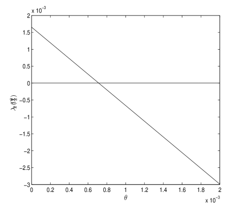
Fig. 1: Smallest eigenvalue of observability Gramian $\Omega_{2}^{\theta}$ for $0\leq\theta\leq 2\times 10^{-3}$.

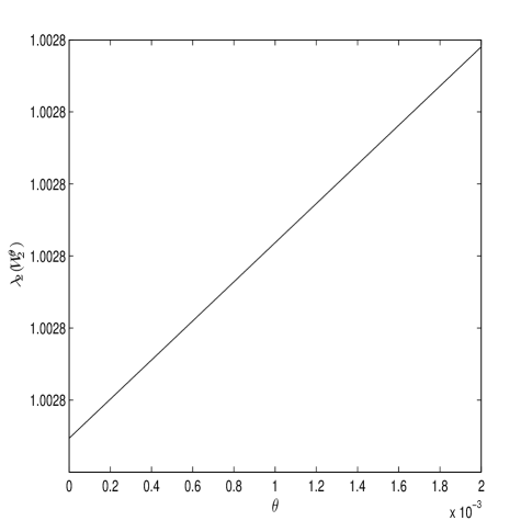
Fig. 2: Smallest eigenvalue of reachability Gramian $W_{2}^{\theta}$ for $0\leq\theta\leq 2\times 10^{-3}$.

Next, to evaluate $\beta_{\rho}$, we observe that with the gain matrix

$$G=\left[\begin{array}[]{c}-13.1\\ -14.4\end{array}\right]$$ (90)

the closed-lood matrix

$$A-GC=\left[\begin{array}[]{cc}13.2&-12.1\\ 14.4&-13.2\end{array}\right]$$

is nilpotent, i.e., its eigenvalues are zero. Note however that $G$ is rather large, which reflects the weak observability of the system. In this case, if we select $\rho=2$, the solution $\Sigma_{2}$ of the Lyapunov equation (83) is

$$\Sigma_{2}=10^{3}\left[\begin{array}[]{cc}1.4622&1.5954\\ 1.5954&1.7431\end{array}\right]\>.$$

Its largest eigenvalue is $\lambda_{1}(\Sigma_{2})=3.2042\times 10^{3}$ and from (87), we obtain $\beta_{2}=2.3407\times 10^{-4}$. This bound is significantly smaller than $\tau_{2}$. To illustrate Lemma 5, the risk-sensitive Riccati iteration $P_{t+1}=r^{\theta}(P_{t})$ is simulated with $\theta=\beta_{2}$ and initial condition $P_{0}=\Sigma_{2}$. The two eigenvalues of $P_{t}$ and $V_{t}$ are plotted as a function of $t$ for $0\leq t\leq 10$ in Fig. 3 and Fig. 4, respectively. As expected, the eigenvalues remain positive and are monotone decreasing. The monotone decreasing property of the eigenvalues is due to the fact that if two $n\times n$ positive definite matrices $P$ and $Q$ are such that $P\geq Q$ and if the eigenvalues of $P$ and $Q$ are sorted in decreasing order, then $\lambda_{i}(P)\geq\lambda_{i}(Q)$ for $1\leq i\leq n$. In other words, the eigenvalues follow the partial order of positive definite matrices. Since according to Lemma 5, the sequence $P_{t}$ is monotone decreasing, so are its eigenvalues. The figures indicate that the risk-sensitive Riccati equation converges very quickly, after 4 or 5 iterations. Note that if $P$ denotes the limit of $P_{t}$, its smallest eigenvalue is $1.003$, but the other eigenvalue is much larger and equals $332.4$. This reflects our earlier observation that one of the modes of the system is barely observable. The eigenvalues of the matrix $A-KC$ for the estimation error dynamics are $0.034$ and $0.776$, so the filter is stable, as expected.

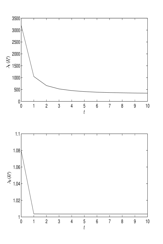
Fig. 3: Eigenvalues of Riccati solution $P_{t}$ for $0\leq t\leq 11$ with $\theta=\beta_{2}$ and initial condition $P_{0}=\Sigma_{2}$.

Fig. 4: Eigenvalues of $V_{t}$ for $0\leq t\leq 11$ with $\theta=\beta_{2}$ and initial condition $P_{0}=\Sigma_{2}$.

Finally, to illustrate the onset of breakdown as $\theta$ increases, the two eigenvalues of the fixed point solution $P^{\theta}$ of $r^{\theta}$ and of the corresponding matrix $V^{\theta}=((P^{\theta})^{-1}-\theta I_{2})^{-1}$ are plotted as a function of $\theta$ in Fig. 5 and Fig. 6, respectively, for $0\leq\theta\leq 0.95\times 10^{-3}$. It is known [10, p. 379] that $P^{\theta}$ is a monotone increasing function of $\theta$, and as expected the eigenvalues of $P^{\theta}$ are monotone increasing. However, while the change in the smaller eigenvalue is barely noticeable, the eigenvalue representing the weakly observable mode increases rapidly with $\theta$. As $\theta$ increases, the eigenvalues of $V^{\theta}$ start diverging, and the breakdown value of $\theta$ for this example is just above $0.95\times 10^{-3}$. This value is significantly higher than the bound $\beta_{2}$ obtained by applying Lemma 5 with the gain (90), suggesting that the bound can be improved. In fact, an exhaustive search over $G$ and $\rho$ showed that $\beta_{\rho}$ is maximized by selecting

$$G=\left[\begin{array}[]{c}-7.2196\\ -7.9753\end{array}\right]$$

and $\rho=1.2849$, in which case $\beta_{\rho}=0.4824\times 10^{-3}$.

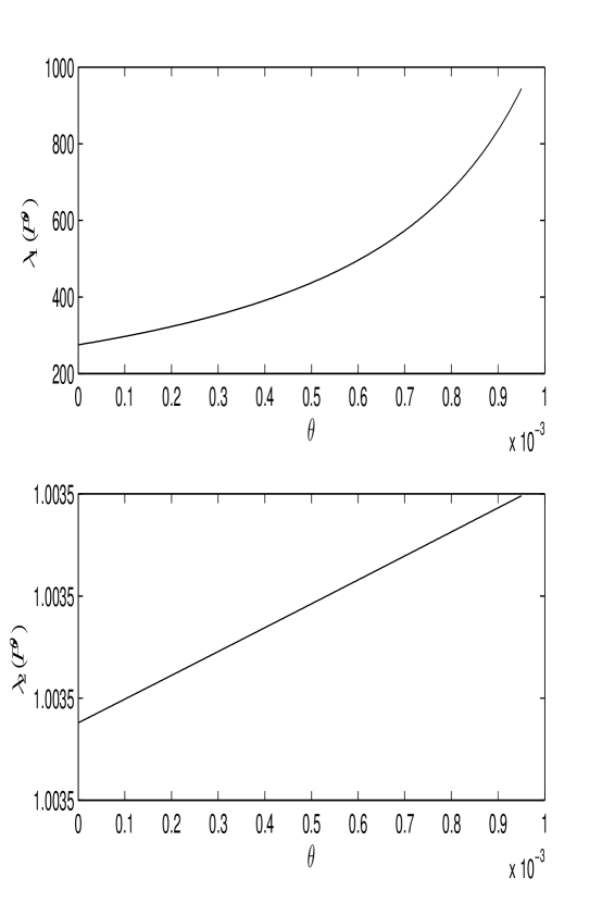
Fig. 5: Eigenvalues of Riccati fixed point $P^{\theta}$ in function of $\theta$ for $0\leq\theta\leq 0.95\times 10^{-3}$.

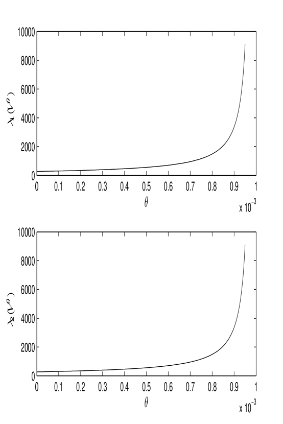
Fig. 6: Eigenvalues of $V^{\theta}$ in function of $\theta$ for $0\leq\theta\leq 0.95\times 10^{-3}$.

7 Conclusions

A convergence analysis of risk-sensitive filters has been presented. It relies on extending Bougerol’s contraction analysis of risk-neutral Riccati equations to the risk-sensitive case. This was accomplished by considering a block-filtering implementation of the $N$-fold Riccati map and showning that this map is strictly contractive as long as an observability Wronskian depending on the risk-sensitivity parameter remains positive definite. A second condition was derived for the risk-sensitivity parameter and initial error variance to ensure that the trajectory of the risk-sensitive Riccati iteration stays positive definite at all times. The two conditions obtained can be viewed as multivariable versions of conditions obtained earlier by Whittle [23, Chap. 9] for the scalar case.

Although the results we have presented concern filters with a constant risk-sensitivity parameter $\theta$, a closely related class of robust filters was derived recently [19] by assigning a fixed relative entropy tolerance to increments of the state-space model. In this case, the risk-sensitivity parameter is time-varying, but the tolerance is fixed, and based on computer simulations, it appears that the risk-sensitivity parameter and associated filter always converge as long as the relative entropy tolerance remains small. Since Bougerol’s analysis [5] is applicable to systems with random fluctuations, it is reasonable to wonder if the analysis presented here can be extended to establish the convergence of the filters discussed in [19].

References

- [1] B. D. O. Anderson and J. B. Moore, Optimal Filtering, Prentice-Hall, Englewood Cliffs, NJ, 1979.
- [2] J. P. Aubin and I. Ekeland, Applied Nonlinear Analysis, J. Wiley, New York, 1984.
- [3] R. N. Banavar and J. L. Speyer, Properties of risk-sensitive filters/estimators, IEE Proc.-Control Theory Appl., 145 (1998).
- [4] R. Bhatia, On the exponential metric increasing property, Linear Algebra and its Appl., 375 (2003), pp. 211–220.
- [5] P. Bougerol, Kalman filtering with random coefficients and contractions, SIAM J. Control and Optimiz., 31 (1993), pp. 942–959.
- [6] R. Davies, P. Shi, and P. Wiltshire, New upper solution bounds of the discrete algebraic Riccati matrix equation, J. Computational and Applied Math., 213 (2008), pp. 307–317.
- [7] L. P. Hansen and T. J. Sargent, Robustness, Princeton University Press, Princeton, NJ, 2008.
- [8] B. Hassibi, A. H. Sayed, and T. Kailath, Linear estimation in Krein spaces. I. Theory, IEEE Trans. Automat. Control, 41 (1996), pp. 18–33.
- [9] , Linear estimation in Krein spaces. II. Applications, IEEE Trans. Automat. Control, 41 (1996), pp. 34–49.
- [10] , Indefinite-Quadratic Estimation and Control– A Unified Approach to and Theories, Soc. Indust. Appl. Math., Philadelphia, 1999.
- [11] M. Ito, Y. Seo, T. Yamazaki, and M. Yanagida, Geometric properties of positive definite matrices cone with respect to the Thompson metric, Linear Algebra and its Appl., 435 (2011).
- [12] T. Kailath, Linear Systems, Prentice Hall, Englewood Cliffs, NJ, 1980.
- [13] T. Kailath, A. H. Sayed, and B. Hassibi, Linear Estimation, Prentice Hall, Upper Saddle River, NJ, 2000.
- [14] R. E. Kalman and R. S. Bucy, New results in filtering and prediction theory, Trans. ASME, Series D, J. Basic Eng., 83 (1961), pp. 95–107.
- [15] S. W. Kim and P. G. Park, Matrix bounds of the discrete ARE solution, Systems Control Letters, 36 (1999), pp. 15–20.
- [16] J. Lawson and Y.Lim, The symplectic semigroup and Riccati differential equations, J. Dynamical and Control Syst., 12 (2006), pp. 49–77.
- [17] , A Birkhoff contraction formula with applications to Riccati equations, SIAM J. Control and Optimiz., 46 (2007), pp. 930–951.
- [18] H. Lee and Y. Lim, Invariant metrics, contractions and nonlinear matrix equations, Nonlinearity, 2 (2008), pp. 857–878.
- [19] B. C. Levy and R. Nikoukhah, Robust state-space filtering under incremental model perturbations subject to a relative entropy tolerance, IEEE Trans. Automat. Control, 58 (2013), pp. 682–695.
- [20] A.-P. Liao, G. Yao, and X.-F. Duan, Thompson metric method for solving a class of nonlinear matrix equations, Applied Math. and Computation, 216 (2010), pp. 1831–1836.
- [21] J. L. Speyer, J. Deyst, and D. H. Jacobson, Optimization of stochastic linear systems with additive measurement and process noise using exponential performance criteria, IEEE Trans. Automat. Control, 19 (1974), pp. 358–366.
- [22] J. L. Speyer, C.-H. Fan, and R. N. Banavar, Optimal stochastic estimation with exponential cost crireria, in Proc. 31st IEEE Conf. Decision Control, Tucson, AZ, Dec. 1992, pp. 2293–2298.
- [23] P. Whittle, Risk-sensitive Optimal Control, J. Wiley, Chichester, England, 1980.