Probing QCD Phase Structure using Baryon Multiplicity Distribution

Abstract

We propose a new method to construct canonical partition functions of QCD from net number distributions such as the net-baryon, net-charge and net-strangeness, by using only the CP symmetry. To demonstrate the method, we apply it to the net-proton number distribution $P_{n}$ recently measured at RHIC. We show that both $\mu/T$ and the canonical partition functions $Z_{n}$ are determined by using the CP invariance $Z_{n}=Z_{-n}$. Comparing $\mu/T$ obtained from the present analysis for the net-proton distribution and that obtained from a thermal statistical model, we find remarkable agreement for wide range of beam energies. Constructing a grand canonical partition function $Z(\mu,T)=\sum_{n}Z_{n}(T)\xi^{n}$, we study moments and Lee-Yang zeros for RHIC data, and discuss possible regions of a phase transition line in QCD. This is the first Lee-Yang zero diagram obtained for RHIC data, which helps us to see contributions of large net-proton data for exploring the QCD phase diagram.

We also calculate $Z_{n}$ by the lattice QCD simulations, and find a clear indication of Roberge-Weiss phase transition in the QGP phase. The method does not rely on the Taylor expansions, which prevent us to go to large $\mu/T$.

1 Introduction

When temperature and density are varied, QCD is expected to have a rich phase structure [1]. One of the most important challenges in particle and nuclear physics is to experimentally discover the phases that only appear under extreme conditions and to theoretically understand their nature. Such achievements would not only deepen our understanding of QCD but also extend our knowledge of the early universe and compact stars.

The Relativistic Heavy Ion Collider (RHIC) was built to explore the properties of QCD matter [2]. Recently net-proton multiplicity measurements at RHIC are gaining attention [3, 4] because they provide valuable information about the QCD phase diagram [5]. In these measurements, the colliding energy is varied, and trajectories of the produced hot matter in ($T,\mu_{B}$) plane may pass near the critical region. Event-by-event fluctuations are expected to encompass the critical point, where the correlation length rapidly changes [6, 7, 8]. In particular, conserved quantities such as the charge or baryon number may reveal possible correlations that existed inside the system before hadronization. See Ref.[9] and references therein.

Usually, data obtained at a given colliding energy is assigned with a set of temperature $T$ and chemical potential $\mu$, which are referred to as chemical freeze-out point, due to the success of a thermal statistical model for hadrons in heavy ion collisions [10].

In this paper, we propose a method by which, we can obtain information of the QCD phase diagram not only at the experimental $(T,\mu/T)$ point, but other values of $\mu/T$. This may seem to be magical, but is possible because we take into account all the multiplicities. Basic idea is the use of CP symmetry to extract canonical partition functions from measured number distribution according to a fundamental equation in statistical mechanics. This idea also provides a model independent method to determine $\mu/T$ only using CP symmetry. As we will show later, $\mu/T$ obtained in the present method is consistent with those obtained from the chemical freeze-out data, for wide range of colliding energies.

In addition, even without direct lattice QCD calculations in physical chemical potential regions, we can calculate the canonical partition functions, which helps us to understand the QCD at the finite density. The method provides us an approach beyond the Taylor expansion method, namely it is possible to calculate large $\mu/T$ regions.

In section 2, we describe how to extract the canonical partition functions, $Z_{n}$, from experimental data, and show the obtained results. In section 3, we construct the grand partition function $Z(\mu,T)$ from these $Z_{n}$, and calculate the moments as a function of $\mu/T$. In section 4, we show that we can calculate the Lee-Yang zero structure from the canonical partition functions obtained by the lattice QCD and the RHIC experiment. To our knowledge, this is the first calculation of the Lee-Yang zero for the high energy nuclear collisions. Section 5 is devoted to the concluding remarks. In Appendix, we give detailed numerical data $Z_{n}$ and Moments $\lambda_{4}/\lambda_{2}$ for RHIC data. Part of the results here were reported in several proceedings [11, 12].

2 Constructing the canonical partition functions

The grand partition function $Z$ and the canonical partition functions $Z_{n}$ are related as

$$Z(\xi,T)=\mbox{Tr}\,e^{-(H-\mu\hat{N})/T}=\sum_{n=-N_{max}}^{+N_{max}}\langle n|e^{-H/T}|n\rangle e^{\mu n/T}=\sum_{n=-N_{max}}^{+N_{max}}Z_{n}(T)\xi^{n},$$ (1)

where $\xi=\exp(\mu/T)$ is fugacity, and

$$Z_{n}=\langle n|\exp(-H/T)|n\rangle.$$ (2)

Here we assume that the number operator $\hat{N}$ commutes with $H$, that is, $\hat{N}$ is a conserved quantity. $\hat{N}$ can be any conserved number operators, such as baryon, charge and strangeness. In the following we consider the baryon number as a concrete example.

Because of the charge-parity symmetry, $Z_{n}$ defined by Eq.(2) satisfy

$$Z_{n}=Z_{-n}.$$ (3)

The multiplicity distributions $P_{n}$ observed in experiments are related to $Z_{n}$ as

$$P_{n}(\xi)=Z_{n}\xi^{n}.$$ (4)

Using Eqs.(3) and (4), we can determine $\xi$ and $Z_{n}$. In Fig.1 and Table 1, we show as an example $P_{n}(\xi)$ and $Z_{n}\xi^{n}$ for $\sqrt{s_{NN}}=39$ GeV[4]. The data correspond to the 0-5% centrality in Au+Au collisions. Here $\xi$=1.88336 as given in Table 1.

Figure2 shows the obtained $\xi$ together with that obtained by freeze-out analysis in Refs.[13] and [14]. Errors in $\xi$ due to the breaking of the relation Eq.(3) are less than one percent for all colliding energies. Note that we use here only the multiplicity data and the charge-parity symmetry relation (3).

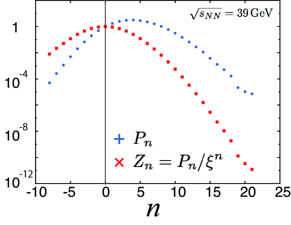
Figure 1: Experimental multiplicity data $P_{n}$, and $Z_{n}=P_{n}/\xi^{n}$ for $\sqrt{s_{NN}}=39$ GeV. $\xi$ is tuned so that $Z_{n}=Z_{-n}$, and $\xi$=1.88336.

We assume that the net-proton multiplicity data are approximately proportional to those of the baryon. This approximation is justified if (i) after the chemical freeze-out, the net-proton number is effectively constant, or (ii) a created fireball is approximately isoneutral. See also Sec.3 in Ref.[15].

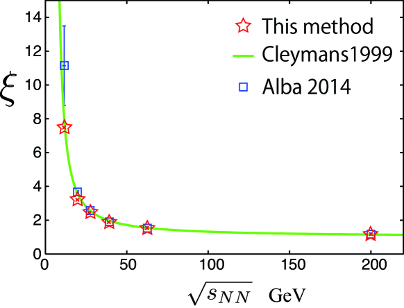
Figure 2: Fugacity $\xi=\exp(\mu/T)$ as a function of the colliding energy $\sqrt{s_{\rm NN}}$. Plotted values are those obtained from RHIC experiments (red star) and the freeze-out results reported in Refs.[13](green line) and [14](blue square).

$\sqrt{s_{NN}}$ GeV	$\xi$ obtained here	Freeze-out (Ref.[13])	Freeze-out (Ref.[14])
11.5	7.48331 $\pm$ 3.85E-6	8.040	11.1 $\pm$ 2.3
19.6	3.20376 $\pm$ 1.504E-2	3.623	3.659 $\pm$ 9.7
27	2.43956 $\pm$ 5.05E-3	2.615	2.573 $\pm$ 2.4
39	1.88336 $\pm$ 1.18E-3	1.981	1.936 $\pm$ 1.8
62.4	1.53377 $\pm$ 2.82E-4	1.551	1.5573 $\pm$ 6.2
200	1.17499 $\pm$ 8.64E-5	1.152	1.1800 $\pm$ 4.8

Table 1: The fugacity $\xi$ at each $\sqrt{s_{NN}}$. The values obtained by the method proposed here are compared with those by the freeze-out analyses.

3 Moments as a function of $\mu/T$ and the QCD transition boundary

From the grand partition function given by Eq.(1), the moments are evaluated using

$$\lambda_{k}(\xi)\equiv\biggl{(}\xi\frac{\partial}{\partial\xi}\biggr{)}^{k}\log Z(\xi).$$ (5)

The quantity $N_{\rm max}$ in Eq.(1) is finite because of the measurement statistics (simulation statistics and finite volume) in the experiments (lattice QCD). The finite nature of $N_{\rm max}$ places an upper bound on the chemical potential for which the calculation is reliable. To estimate the effect of the finite $N_{\rm max}$, we test two cases:

1. the values of the final three $Z_{n}$ ($n=N_{\rm max}-2$, $N_{\rm max}-1$, $N_{\rm max}$) are increased by 15%

2. the final two $Z_{n}$ ($n=N_{\rm max}-1$,  $N_{\rm max}$) are set to zero.

As an example, we plot the number susceptibility $\lambda_{2}/N_{\rm max}$ in Fig.3 as a function of $\mu/T$ at $\sqrt{s_{\rm NN}}=27$ GeV for these two cases together with the one constructed from all the $Z_{n}$.

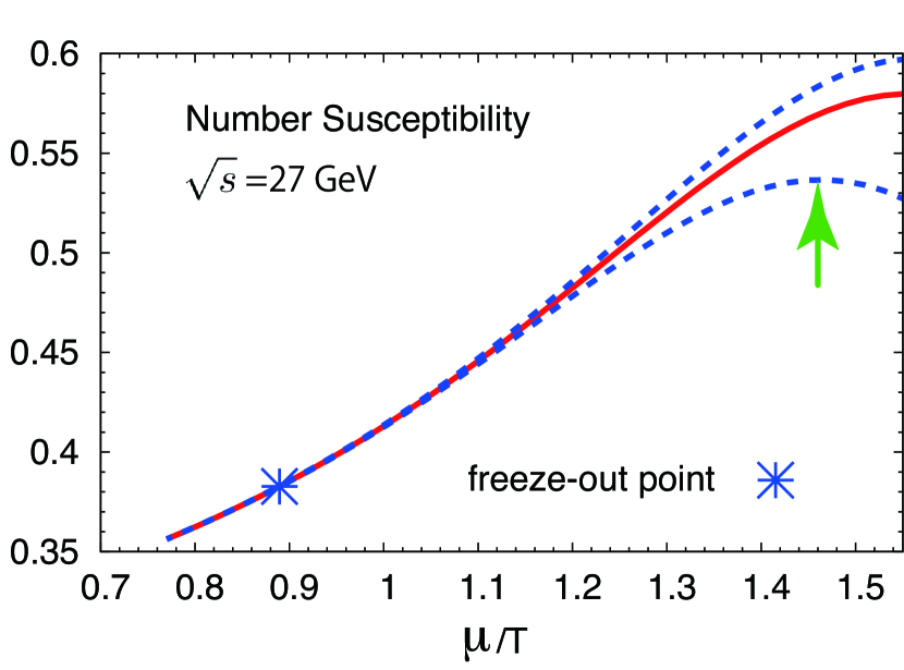
Figure 3: Number susceptibility, $\lambda_{2}/N_{\rm max}$, at $\sqrt{s_{\rm NN}}=27$ GeV as a function of $\mu/T$. The upper curve is obtained by increasing the final three $Z_{n}(n=N_{\rm max}-2,\,N_{\rm max}-1,\,N_{\rm max}$) by 15%. The lower curve results from removing the final two $Z_{n}$ terms.

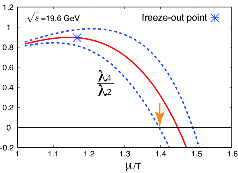
Figure 4: Ratio of the moments $\lambda_{4}/\lambda_{2}$ as a function of $\mu/T$ at $\sqrt{s_{\rm NN}}=$19.6 GeV. The upper and lower curves are constructed by the same procedure as used in Fig.3

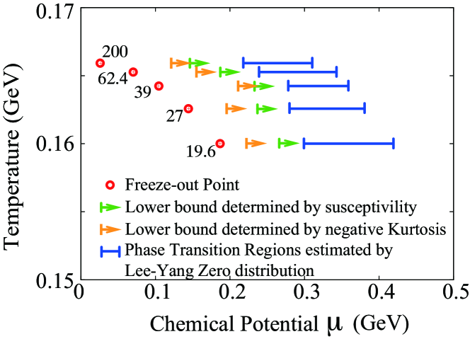
Figure 5: Potential regions of hidden phase transition. The regions are estimated as the complement of areas where no transition is evident.

Let us suppose that, as $\mu$ increases, we encounter a phase transition or a cross-over, and cross it. In this case, we would expect the structure of the moments to be rough in this area. At the peak position of the lower curve, indicated by an arrow in Fig.3, the center line continues to increase. We write this value as $\bar{\mu}(T)$, and any transition may occur for $\mu\geq\bar{\mu}$. In other words, this position $\bar{\mu}$ is a candidate for the lower bound of the real susceptibility peak. We then investigate the behavior of $\lambda_{3}/\lambda_{2}$ and $\lambda_{4}/\lambda_{2}$. Although higher moments have large effects of the finite $N_{\rm max}$, they may be a good tool for detecting the transition region of the QCD phase diagram [6]. The former ratio does not indicates a significant structure for $\mu\leq\bar{\mu}$. Around the freeze-out points, $\lambda_{4}/\lambda_{2}\sim 1$ (Poisson) and it becomes negative as $\mu$ increases. See Fig.4. In Refs.[16, 17, 8], it is argued that a negative value of $\lambda_{4}/\lambda_{2}$ indicates that the phase transition has been reached. We give $\lambda_{4}/\lambda_{2}$ at $\sqrt{s_{NN}}=$ 11.5, 19.6, 27, 39, 62.4 and 200 GeV in the appendix.

We take the points where the lower curve of $\lambda_{4}/\lambda_{2}$ becomes negative (indicated by an arrow in Fig.4) as an another candidate for the lower bound $\bar{\mu}(T)$ and show them in Fig.5.

4 Lee–Yang zero structure

Next we extend the fugacity $\xi$ to complex values. Lee–Yang zeros (LYZs) $\alpha_{l}$ are zeros of the grand partition function $Z(\xi)$ in the complex fugacity plane; that is,

$$Z(\xi)=\prod(\xi-\alpha_{l}).$$ (6)

The distribution of these zeros reflects the phase structure of the corresponding statistical system. Lee and Yang argued that for a finite system, no zeros appear on the real axis. In the thermodynamic limit, the number of zeros becomes infinite and the zeros coalesce onto one-dimensional curves [18]. For the first-order (second-order) phase transition, the coalescing zeros cross (pinch) the real positive $\xi$ axis [19], whereas for the crossover, they do not reach the real axis.

The first pioneering work to calculate the LYZs of the lattice QCD was carried out by Barbour and Bell [20], who found that the zero distribution is considerably different in the confinement and deconfinement phases. In Ref.[21] the authors calculated the LYZs in the complex $\beta=6/g^{2}$ plane to distinguish between a crossover and a second-order phase transition by investigating the volume dependence. Ejiri pointed out that this approach is very difficult with finite statistics since the phase of $\det\Delta(\mu)$ is mixed with the complex $\beta$ [22].

Although there have been many phenomenological approaches to extracting information on the QCD phase [9, 6, 8], no study has yet been carried out to employ experimental data to investigate the QCD phase through the LYZs.

For this purpose it is important to reliably determine the LYZs; that is, all zeros must be found without ambiguity, and their positions in the complex fugacity plane must be determined with high accuracy. We obtain the LYZs as follows. We first map the problem to the calculation of the residue of $Z^{\prime}/Z$:

$${Z^{\prime}}/{Z}=\sum{1}/({\xi-\alpha_{l}}).$$ (7)

The left hand side of Eq.(7) is integrated along a contour, and the residues inside the contour are summed according to Cauchy’s theorem. Because of the symmetry $+\mu\leftrightarrow-\mu$, if $\alpha_{l}$ is a solution, then $1/\alpha_{l}$ is also a solution. Therefore, we only need to search for residues inside the unit circle.

Figure 6 shows the cut Baum-Kuchen (cBK) shape contours used in the study. Starting from $0\leq\theta<2\pi$, and $0<r\leq 1$ in polar coordinates, the region is divided into four pieces, and the Cauchy integral is evaluated over each section. This divide-and-conquer process is iterated as many times as required (here 20 times). When no residue is found in a section, no further divisions are applied to that section. At each divide-and-conquer level, we check the conservation of the residue sum. The technical details of this approach will be presented elsewhere, including the parallelization.

All calculations were performed using the multiple-precision package, FMlib [23] and the number of significant digits was 50 - 100. With this algorithm, we can construct LYZ diagrams from $Z_{n}$.

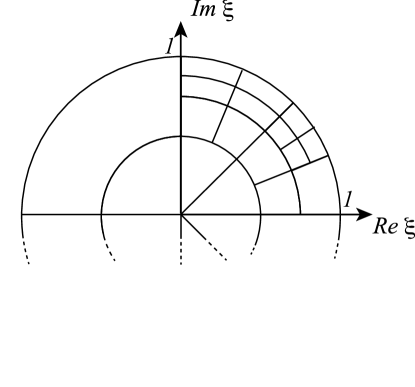
Figure 6: Schematic of the cBK contours in the divide-and-conquer search for residues.

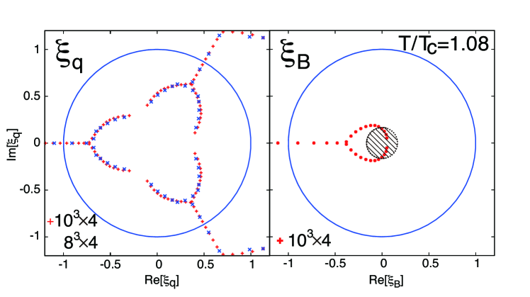
Figure 7: LYZ diagram from the lattice QCD. $T/T_{c}=1.08$ ($\beta=1.9$). Left: The lattice size is $10^{3}\times 4$ and $8^{3}\times 4$ and $N_{\rm max}=28$ and 14, respectively. Right: The same diagram using a lattice size of $10^{3}\times 4$, but now it is displaced in terms of the baryon chemical potential $\xi_{B}$ instead of the quark chemical potential $\xi_{q}$, where $\xi_{B}=\xi_{q}^{3}$. The shaded circle is an area with high density, i.e., $|\xi|\leq\exp(-3*0.6)$, where the lattice QCD results have limited applicability.

4.1 Lattice calculations

First, we study the LYZs obtained by lattice QCD simulation. Here we do not distinguish between $u$ and $d$ quarks. Details of calculating $Z_{n}$ by lattice QCD simulation are given in [24], where the fugacity expansion formula [25] plays an essential role in obtaining $Z_{n}$. We update 11000 trajectories including 3000 thermalization trajectories. The measurement is performed every 10 (20) trajectories for a $8^{3}\times 4(10^{3}\times 4)$ lattice size. A Monte Carlo update is performed with the fermion measure at $\mu=0$; thus, we avoid the sign problem due to the complex fermion determinant. However, an overlap problem may still exist.

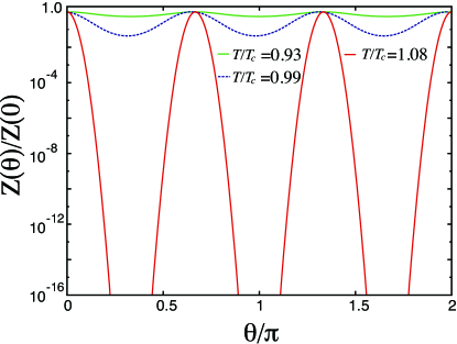
Figure 8: The grand partition function, $Z(\theta)$ as a function of $\theta\equiv\mbox{Im}(\mu)/T$ for $T/T_{c}=1.08,0.99$ and 0.93. Above $T_{c}$, $Z(\theta)$ drops rapidly at $\theta=\pi/3,\pi$ and $5\pi/3$, where the free energy drops rapidly.

The LYZ diagram of the lattice QCD above the phase-transition temperature is shown in Fig.7. For $Z_{n}$, we use data with $(\mbox{signal}/\mbox{noise})\geq 2$. The condition $Z_{n}=0$ for $n=1,2\,(\mbox{mod}\,3)$ is imposed on the lattice data for $Z_{n}$[26, 27] which guarantees $2\pi/3$-translational invariance for $\mbox{Im}(\mu)/T$. We evaluate the LYZs for $Z(\xi_{B})=\sum_{m}Z_{3m}\xi_{B}^{m}$ and map the result onto $\xi=\xi_{B}^{1/3}$.

In Ref.[28] it is shown that two widely used methods, the multi-parameter reweighting and Taylor expansion, are consistent for the EoS and number density up to $\mu_{q}/T\sim$ 0.8 and for number susceptibility up to $\mu_{q}/T\sim$ 0.6. This implies that the current lattice QCD calculation should not be considered reliable in the higher density regions. In the right panel of Fig.7, the circle corresponding to $|\xi|=\exp(-3\mu_{q}/T)$ with $\mu_{q}/T=0.6$ is displayed.

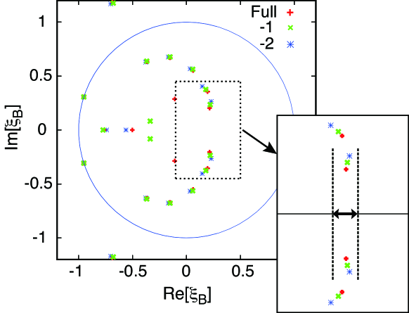
Figure 9: LYZ diagram from RHIC data at $\sqrt{s_{\rm NN}}=200$ GeV. “Full” result is calculated by using all $Z_{n}$. “-1” is calculated by removing a pair with $Z_{n}$ of $n=\pm N_{\rm max}$. For “-2”, we remove further pair of $Z_{n}$. The inset is an enlarged view near the positive real axis, which gives the predicted region of the QCD phase transition in Fig.5.

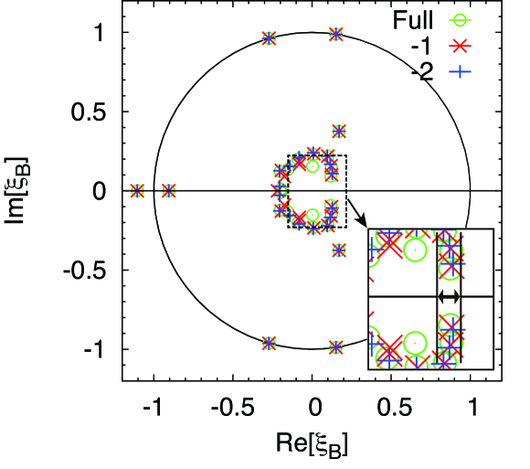
Figure 10: LYZ diagram from RHIC data at $\sqrt{s_{\rm NN}}=19.6$ GeV. “Full”, “-1” and “-2” denote the same as in Fig.9

Because the $Z_{n}$ obtained in the confinement region suffer from significant noise, the LYZ diagram should be considered qualitative. However, despite this, distinctive differences are observed above and below the confinement/deconfinement transition temperature. At $T\sim 1.2T_{c}$, a line of the zero accumulation appears at $\arg(\xi)=\pm\pi/3$, which is consistent with the Roberge-Weiss (RW) phase transition. Of course, in order to confirm this is a real RW phase transition, we must go to large volume (large $N_{max}$) and check that zeros are accumulated.

Roberge and Weiss discussed the regions of pure imaginary chemical potential, and found that at $\mbox{Im}(\mu)/T=\pi/3+2k\pi/3$ ($k=0,1$), a phase transition occurs for $T\geq T_{\rm RW}$ [29]. The transition is the first-order transition above $T_{\rm RW}$, and it is easy to detect at experiments. See Ref.[30] for detailed discussions on the order of the RW phase transition. See Refs.[31, 32] for more detailed discussion how to occur the Roberge-Weisse phase transition.

Using the same lattice setup as that in the present study, the quantity $T_{\rm RW}$ was estimated to be approximately $1.1T_{c}$ [33]. This phase transition exerts a clear effect on the LYZ diagram at $T\sim 1.2T_{c}$, while no such effect appears at $T\lesssim T_{c}$.

The fugacity, $\xi$, on the unit circle stands for the pure imaginary chemical potential. The relation between the pure imaginary, zero and real chemical potential are discussed in Refs.[34, 35].

In the left panel of Fig.9, we check the volume dependence by plotting $8^{3}\times 4$ and $10^{3}\times 4$ cases; here $N_{max}$ is chosen so that $N_{max}/V$ is approximately the same for $V=10^{3}$ and $8^{3}$. In this simulation, $N_{max}/V\sim 1.7\mbox{ fm}^{-3}$, i.e., in a cube with one $fm$ on a side, up to $3\times 1.7$ quarks are included. See Ref.[36], where the authors estimate $N_{max}/\sqrt{V}$ for obtaining reliable results as a function of the temperature based on the quark-meson model.

Using the relation,

$$Z=\sum Z_{n}\xi^{n},$$ (8)

we can see the behavior of the grand partition function, $Z(\xi=\exp(\mu/T))$, for the pure imaginary chemical potential. We show this behavior in Fig.8 for several temperatures. Lee and Yang pointed out that phase transition regions correspond to zeros of the grand partition function. In Fig.8, such characteristic behaviors are observed at the Roberge-Weiss phase transition points in the pure imaginary chemical potential above $T_{c}$. As a consequence, the thermo potential changes rapidly. Because our $N_{max}$ is finite, exact Lee-Yang zeros do not appear on the pure imaginary chemical potential. However, rapid decrease of $Z(\theta)$ is seen. Since

$$Z_{n_{q}}=0\quad\quad\mbox{for}\quad n_{q}=1,2\quad(\mbox{mod}\quad 3)$$ (9)

where $n_{q}$ are the quark number. The symmetry of

$$Z(\theta)=Z(\theta+\frac{2\pi}{3})$$ (10)

leads to the relation (9).

Whether zeros appear in Eq.(8) on the pure imaginary regions, i.e. on the unit circle in the complex fugacity plane, or not depends on the nature of $Z_{n}$. In other words, whether the Roberge Weise phase transition occurs or not is the outcome of the dynamics. In Ref.[32], an explicit example of $Z_{n}$ that leads to Roberge Weiss phase transition above $T_{c}$ is given and its mechanism is explained.

4.2 Relativistic Heavy Ion Collisions

We next consider the LYZ diagrams obtained from RHIC data. We construct the grand partition function Eq.(1) for $\sqrt{s_{\rm NN}}=$ 19.6, 27, 39, 62.4 and 200 GeV from the data for which $P_{n}\geq 2$, and use the cBK method to calculate the LYZ diagrams. The results for $\sqrt{s_{\rm NN}}=$200 and 19.6 GeV are shown in Fig.9 and 10. To clarify the effect of a finite $N_{\rm max}$, we also calculate the LYZs while neglecting $Z_{n}$ for $n=\pm N_{\rm max}$ (“-1”) and while neglecting $Z_{n}$ for $n=\pm N_{\rm max}$ and $\pm(N_{\rm max}-1)$ (“-2”).

Although some zeros exist on the negative real axis, they do not form a line that clearly characterizes the RW transition, which suggests that the data correspond to temperatures below $T_{\rm RW}$. Remember that the net-proton number is not an exactly conserved quantity. It is therefore very interesting to construct the Lee-Yang zeros and to study their structure for the conserved charge, such as net charge or strangeness.

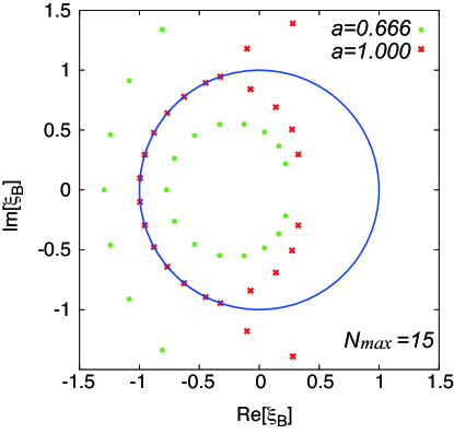
Figure 11: LYZ diagram of the Skellam distribution, in which $Z_{n}$ are given by $I_{n}(a)$. (green) $a=6.66$ which corresponds to $\sqrt{s_{\rm NN}}=200$ GeV Star experiment; (red) $a=10$. In both cases, $N_{\rm max}$ is set to be 15, as in Fig. 9

In the LYZ diagrams obtained from the RHIC data, no zero appears on the positive real-$\xi$ axis. Possible explanations for this result are that (i) there is no phase transition, but a crossover occurs at these temperatures, (ii) the systems are finite, and/or (iii) the $N_{\rm max}$ values are too small. The size of the fireball produced is comparable to the QCD scale, and thus, explanation (ii) is at least partially correct. To further explore the QCD phase transition, a larger $N_{\rm max}$ must be attained.

Several LYZ points appear on the unit circle for the all RHIC data. To understand the meaning of this, we calculate the LYZ diagram for the Skellam model. This is a simple probabilistic model based on the difference between two Poisson distribution variables $N_{1}$ and $N_{2}$, and in our case $Z_{n}=I_{n}(a)$. See Ref.[37]. Here $I_{n}$ is the modified Bessel function; the parameter $a$ is unique, once the averages of $N_{1}$ and $N_{2}$ are given. In Fig.11, the points with $a=0.666$ corresponds to the multiplicity in the case of $\sqrt{s_{\rm NN}}=200$ GeV. Two circles appear inside and outside of the unit circle, and no LYZ point on the unit circle. However, if we increase $a$ artificially, the two circles move closer to the unit circle and several points coalesce on the unit circle. This indicates that a gross feature of the RHIC multiplicity data is configured by the probabilistic origin, but the LYZ distribution includes additional information on the QCD dynamics.

Finally, we estimate where the LYZs would intercept or approach the positive real axis as the volume increases, which indicates the QCD phase transition. These zones are indicated by double -headed arrows in the inset of Fig.9. In Fig.5, the corresponding regions are indicated by horizontal lines. If the multiplicities $P_{n}$ with larger $n$ were to be measured in future experiments, the QCD phase transition could be pinpointed with more precision. Further study of the relation between the baryon and proton number distributions will improve the analysis here [38].

5 Concluding Remarks

A simple but important relation discussed in this paper is

$$Z(\mu,T)=\sum_{-N_{max}}^{N_{max}}Z_{n}(T)\xi^{n},$$ (11)

e.g., the fugacity expansion of the grand partition function $Z$ with the coefficients $Z_{n}$, which are the canonical partition functions.

We have shown how to construct $Z_{n}$ from experimental net-multiplicities. In high energy heavy ion central collision, a fireball with $\mu$ and $T$ is a good picture, at least as a global feature. Then the selection of an event with a net-multiplicity is a filter of $Z_{n}$.

In lattice QCD simulation, we consider the path integral formula of the grand partition function,

$$Z(\mu,T) = \int\mathcal{D}U(\det D(\mu))^{N_{f}}e^{-S_{G}}$$ (12)

$$= \int\mathcal{D}U\frac{(\det D(\mu))^{N_{f}}}{(\det D(0))^{N_{f}}}(\det D(0))^{N_{f}}e^{-S_{G}},$$ (13)

where $\det D$, $N_{f}$ and $S_{G}$ are fermion determinant, the number of flavor and gluon action, respectively. We expand $\det D(\mu)$ in a fugacity series. Then we get a formula (11).

The canonical partition functions, $Z_{n}$, depend on only the temperature $T$, but not on the chemical potential $\mu$. Therefore once we extract $Z_{n}$ from $Z(\mu,T)$, we can evaluate $Z$ at different values of $\mu^{\prime}$.

This is very important for exploring the QCD phase boundary: So far, analyses such as the moments have been done on the freeze-out points. But the freeze-out points realized in the BES experiments are in the confinement regions, and not very near to the phase transition. Indeed, Fukushima estimated the baryon density on the freeze-out line using the hadron resonance gas model, and found that the maximum of the baryon density is realized at $\sqrt{s_{NN}}=8$ GeV, but its value is only slightly larger than the normal nuclear density $\rho_{0}$[39]. Using our formula, (11), we can probe higher chemical potential regions from $Z_{n}$ constructed at the chemical freeze-out point.

We calculated the moments (5), and saw their behavior when increasing $\mu/T$. We checked the effects of the finite $N_{max}$.

The formula (11) makes it possible to calculate $Z(\mu,T)$ at complex values of $\mu$. We studied the Lee-Yang zero distribution data of both the experiments and the lattice simulations. To our knowledge, this is the first Lee-Yang zero analysis of the RHIC data. Lattice results told us that the zeros corresponding to Roberge-Weiss transitions appear above $T_{c}$. We did not see such structure in the LYZ of RHIC data. This suggests that these experimental data are produced below $T_{\rm RW}$, where $T_{\rm RW}$ is Roberge-Weiss transition temperature that is around $1.1T_{c}$.

There were claims that the RW transition formulated in the Euclidean space can not be interpreted as a physics object in the Minkowski space by considering its cosmological consequences [40, 41]. In this paper, we discussed the relation between the RW phase transition and the high energy heavy ion experiment, which hopefully advance understanding of the QCD phase diagram .

The approach investigated here is based on the simple statistical mechanics, and is easy to use for extracting information from experimental data. It works equally in analyzing experimental data and lattice QCD simulations. In the latter case, we can study the real chemical potential regions without Taylor expansions.

Several problems that should be clarified in future are

• We can study finite real chemical potential regions in lattice QCD simulation and the sign problem does not appear here. A possible obstacle is the overlap problem. In our lattice Monte Carlo simulations, the gauge configurations are produced at $\mu=0$ as in Eq.(13). Such configurations may not overlap enough with states of large $n$. The canonical partition functions $Z_{n}$ are given in

  $$Z_{n}=\int_{-\pi}^{+\pi}\frac{d\theta}{2\pi}Z(\theta\equiv\mu_{I}/T)e^{i\theta n},$$ (14)

  where $\mu_{I}$ is pure imaginary chemical potential. In other words, $Z(\xi)$ on the unit circle has whole information . On this circle, $\det D$ is real, and the Monte Carlo simulation is possible. Therefore, in addition to $\mu=0$, more points on the unit circle may improve the overlap problem.

• Since $(\det D(\mu))^{2}$ is real positive on the unit circle in $\xi$ plane, $Z(\xi)$ cannot be zero. Therefore Lee-Yang zeros on the unit circle are artifact of $N_{max}$, or the $u-$ and $d-$ quark contribution, $\det D(\mu_{u})\det D(\mu_{d})$ gives such a effect. Therefore we need larger $N_{max}$ both in experiments and lattice QCD calculations.

• It is difficult to measure experimentally the net baryon multiplicity. One possible approach is to study the difference between net-proton multiplicity and net-baryon multiplicity.

• Net strangeness and net charge multiplicity are analyzed in the same way.

• The relation between the order of the RW transition and the Lee-Yang zeros should be studied more quantitatively near the end-point. The volume dependence of Lee-Yang zeros in the vicinity of a transition point depends on the order of the transition. If the transition is the second order, Lee-Yang zeros approach the RW phase points according to the volume dependence with a critical exponent.

• The Lee-Yang zeros calculated in the lattice QCD simulation at high temperature suggest the RW transition. But there might be danger to misidentify the thermal singularity with the Lee-Yang zeros. The former appears as a branch point at $\xi=e^{-m_{N}/T}$ inside the unit circle and a cut to $-\infty$ on real negative $\xi$ axis [34, 17]. In order to avoid such misidentification, it is important to check the volume dependence.

• The Lee-Yang zeros are closing to the real positive axis if the system indicates the phase transition. Therefore it is interesting the volume dependence of the Lee-Yang zeros. Such information may be obtained by varying the atomic number of beam/target.

• Recently, based on the canonical partition functions, detailed analyses of effects of $N_{max}$ on the Lee-Yang zeros and the RW transition were reported, using the random matrix model and the saddle point approximation [42, 43]. It is valuable to repeat calculations presented in this paper with referring these analyses.

• Both experimental and lattice QCD data include errors. It is important to check whether obtained Lee-Yang zeros are stable or not against these errors, since it requires extreme care to calculate zeros of high order polynomials. In lattice QCD, we have investigated statistical errors of Lee-Yang zeros caused by statistical error of $Z_{n}$ by using a bootstrap analysis. We found that the Lee-Yang zeros of high temperature QCD are stable near the unit circle on the fugacity plane [32]. If errors of $P_{n}$ are available, we can investigate the error of Lee-Yang zeros for experimental data in a similar manner to lattice QCD. In Ref. [44], the authors addressed the numerical error of Lee-Yang zeros using a random matrix model with finite chemical potential. They calculated zeros of the grand partition function in the complex $\mu$ and observed their behavior when they change the exact polynomial coefficients, $c_{k}$ to $\tilde{c}_{k}$ as $\tilde{c}_{k}=c_{k}(1+R_{k}\epsilon)$ . Here $R_{k}$ are random numbers between $[-1,1]$. They found that the deviation of the zeros on the real $\mu$ axis from the exact values is approximately proportional to $\log\epsilon$, and that the structure os Lee-Yang zeros is not spoiled.

Appendix A Canonical partition functions, $Z_{n}$ for RHIC data

In this appendix, we give $Z_{n}$ obtained in Sec.2. Since $Z_{-n}=Z_{n}$, we show only $n\geq 0$ values. The data are normalized as $Z_{0}=1$ at each energy. $\Delta Z_{n}$ are estimated errors.

$n$	$Z_{n}$	$\Delta Z_{n}$
0	0.10000E+01	0.62112E-07
1	0.62361E+00	0.69741E-07
2	0.33222E+00	0.66895E-07
3	0.12597E+00	0.45672E-07
4	0.40292E-01	0.26301E-07
5	0.10419E-01	0.12245E-07
6	0.23949E-02	0.50681E-08
7	0.46882E-03	0.17863E-08
8	0.83546E-04	0.57315E-09
9	0.13110E-04	0.16194E-09
10	0.18749E-05	0.41698E-10
11	0.24529E-06	0.98222E-11
12	0.29522E-07	0.21285E-11
13	0.32786E-08	0.42561E-12
14	0.33756E-09	0.78901E-13
15	0.33251E-10	0.13994E-13
16	0.30000E-11	0.22732E-14
17	0.26163E-12	0.35694E-15
18	0.21094E-13	0.51818E-16
19	0.15816E-14	0.69954E-17
20	0.11258E-15	0.89653E-18
21	0.83712E-17	0.12003E-18
22	0.56668E-18	0.14630E-19
23	0.38519E-19	0.17905E-20
24	0.18180E-20	0.15215E-21
25	0.70247E-22	0.10585E-22
26	0.82136E-23	0.22285E-23
27	0.31360E-24	0.15320E-24
28	0.34922E-25	0.30717E-25

Table 2: $\sqrt{s_{NN}}$=11.5 GeV

$n$	$Z_{n}$	$\Delta Z_{n}$
0	0.10000E+01	0.11360E-01
1	0.88457E+00	0.16150E-01
2	0.65521E+00	0.19945E-01
3	0.40203E+00	0.19813E-01
4	0.20550E+00	0.14453E-01
5	0.90348E-01	0.11442E-01
6	0.34569E-01	0.70907E-02
7	0.11665E-01	0.38755E-02
8	0.35214E-02	0.18949E-02
9	0.96801E-03	0.84371E-03
10	0.23849E-03	0.33668E-03
11	0.54473E-04	0.12456E-03
12	0.11384E-04	0.42160E-04
13	0.22056E-05	0.13231E-04
14	0.40106E-06	0.38968E-05
15	0.67442E-07	0.10614E-05
16	0.10994E-07	0.28023E-06
17	0.16066E-08	0.66333E-07
18	0.21451E-09	0.14345E-07
19	0.27632E-10	0.29929E-08
20	0.39570E-11	0.69420E-09
21	0.46594E-12	0.13240E-09
22	0.46170E-13	0.21250E-10
23	0.57645E-14	0.42973E-11

Table 3: $\sqrt{s_{NN}}$=19.6 GeV

$n$	$Z_{n}$	$\Delta Z_{n}$
0	0.10000E+01	0.55468E-02
1	0.90362E+00	0.83594E-02
2	0.68168E+00	0.10515E-01
3	0.43157E+00	0.10829E-01
4	0.23245E+00	0.95400E-02
5	0.10813E+00	0.73858E-02
6	0.44216E-01	0.58895E-02
7	0.15962E-01	0.30883E-02
8	0.52022E-02	0.16718E-02
9	0.15312E-02	0.81733E-03
10	0.41235E-03	0.36560E-03
11	0.10014E-03	0.14748E-03
12	0.22725E-04	0.55589E-04
13	0.47693E-05	0.19378E-04
14	0.93667E-06	0.63214E-05
15	0.16794E-06	0.18826E-05
16	0.30799E-07	0.57346E-06
17	0.47106E-08	0.14569E-06
18	0.69913E-09	0.35914E-07
19	0.11524E-09	0.98328E-08
20	0.93232E-11	0.13213E-08
21	0.17834E-11	0.41984E-09

Table 4: $\sqrt{s_{NN}}$=27 GeV

$n$	$Z_{n}$	$\Delta Z_{n}$
0	0.10000E+01	0.20603E-02
1	0.91388E+00	0.29289E-02
2	0.69779E+00	0.34996E-02
3	0.45149E+00	0.35006E-02
4	0.25020E+00	0.30516E-02
5	0.12024E+00	0.22448E-02
6	0.50805E-01	0.14914E-02
7	0.19122E-01	0.93227E-03
8	0.64636E-02	0.51254E-03
9	0.19762E-02	0.22024E-03
10	0.54891E-03	0.95311E-04
11	0.14064E-03	0.38048E-04
12	0.32779E-04	0.13816E-04
13	0.73396E-05	0.48197E-05
14	0.15625E-05	0.15986E-05
15	0.28234E-06	0.45005E-06
16	0.50870E-07	0.12634E-06
17	0.10789E-07	0.41746E-07
18	0.18428E-08	0.11109E-07
19	0.12762E-09	0.11987E-08
20	0.33882E-10	0.49581E-09
21	0.11993E-10	0.27344E-09

Table 5: $\sqrt{s_{NN}}$=39 GeV

$n$	$Z_{n}$	$\Delta Z_{n}$
0	0.10000E+01	0.47305E-03
1	0.92168E+00	0.79653E-03
2	0.72216E+00	0.11385E-02
3	0.48191E+00	0.13929E-02
4	0.27792E+00	0.14614E-02
5	0.14035E+00	0.13333E-02
6	0.62429E-01	0.11101E-02
7	0.24831E-01	0.78510E-03
8	0.89221E-02	0.51745E-03
9	0.28887E-02	0.33828E-03
10	0.86915E-03	0.15845E-03
11	0.23370E-03	0.83409E-04
12	0.60694E-04	0.39564E-04
13	0.14052E-04	0.16730E-04
14	0.30132E-05	0.65523E-05
15	0.56945E-06	0.22616E-05
16	0.10396E-06	0.75408E-06
17	0.26627E-07	0.35277E-06
18	0.47347E-08	0.11457E-06

Table 6: $\sqrt{s_{NN}}$=62.4 GeV

$n$	$Z_{n}$	$\Delta Z_{n}$
0	0.10000E+01	0.16546E-03
1	0.92030E+00	0.26094E-03
2	0.72070E+00	0.35016E-03
3	0.48388E+00	0.40286E-03
4	0.28066E+00	0.40041E-03
5	0.14265E+00	0.34875E-03
6	0.63967E-01	0.26797E-03
7	0.25682E-01	0.18436E-03
8	0.93739E-02	0.11531E-03
9	0.30591E-02	0.64484E-04
10	0.95799E-03	0.34604E-04
11	0.24394E-03	0.15099E-04
12	0.57285E-04	0.60760E-05
13	0.18142E-04	0.32974E-05
14	0.31923E-05	0.99425E-06
15	0.92947E-06	0.49606E-06

Table 7: $\sqrt{s_{NN}}$=200 GeV

Appendix B Moments $\lambda_{4}/\lambda_{2}$ for RHIC data

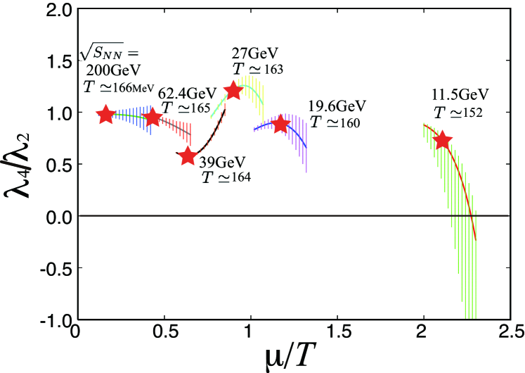
Figure 12: The ratio of the moments $\lambda_{4}$ and $\lambda_{2}$, which correspond $\kappa\sigma^{2}/T^{2}$ as a function of $\mu/T$ for RHIC beam energy scan data at $\sqrt{s_{NN}}=$11.5, 19.6, 27, 39, 62.4 and 200 GeV. Here $\kappa$ and $\sigma^{2}$ are the kurtosis and the variance, respectively. The red starts indicate the freeze-out points.

References

- [1] K. Fukushima and T. Hatsuda, Rep. Prog. Phys. 74:014001, 2011.
- [2] M. Gyulassy and L. McLerran, Nucl. Phys. A750: 30, 2005.
- [3] M. M. Aggarwal et al., Phys. Rev. Lett. 105 022302 (2010).
- [4] X. Luo, Nucl. Phys. A904 (2013) 911c.
- [5] M. A. Stephanov, K. Rajagopal, and E. V. Shuryak. Phys. Rev. Lett. 81, 4816 (1998).
- [6] B. Friman, F. Karsch, K. Redlich and V. Skokov, Euro. Phys. J. C(2011) 71: 1694.
- [7] C. Athanasiou,K. Rajagopal and M. Stephanov, Phys. Rev. D 82, 074008 (2010).
- [8] M. A. Stephanov, Phys. Rev. Lett. 107, 052301 (2011).
- [9] K. Morita et al., Eur.Phys.J. C74 (2014) 2706.
- [10] P. Braun-Munzinger , K. Redlich and J. Stachel, Quark Gluon Plasma 3, 491, Eds. R. Hwa and X.N. Wang, World Scientific, Singapore, 2004.
- [11] A. Nakamura and K. Nagata, JPS Conference Proceedings Volume 1, 016002.
- [12] A. Nakamura and K. Nagata, Nucl. Phys. A931, (2014) pp. 825-830, Proceedings of QUARK MATTER 2014.
- [13] J. Cleymans et al., H. Oeschler, K. Redlich and S. Wheaton Phys. Rev. C73, 034905 (2006).
- [14] P. Alba et al., arXiv:1403.4903 [hep-ph]
- [15] Xiaofeng Luo, Acta Physica Polonica B Proceedings Supplement 5 (2012) 497.
- [16] R. V. Gavai and S. Gupta, Phys. Lett. B696 459, 2011.
- [17] V. Skokov et al., Phys. Rev. C83, 054904,2011.
- [18] C. N. Yang and T. D. Lee, Phys. Rev. 87, 404 (1952), T. D. Lee and C. N. Yang, Phys. Rev. 87 410(1952).
- [19] M. A. Stephanov, Phys. Rev. D73, 094508 (2006).
- [20] I.M. Barbour and A.J. Bell, Nucl. Phys. B372 (1992) 385.
- [21] Z. Fodor and S. Katz, JHEP 04 (2004) 050.
- [22] S. Ejiri, Phys. Rev. D 73, 054502 (2006).
- [23] D. M. Smith, http://myweb.lmu.edu/dmsmith/FMLIB. html.
- [24] K. Nagata et al., Prog. Theor. Exp. Phys. 2012: 1A103.
- [25] K. Nagata and A. Nakamura, Phys. Rev. D82 094027.
- [26] A. Hasenfratz and D. Toussaint, Nucl. Phys. B371 (1992) 539.
- [27] S. Kratochvila and Ph. de Forcrand, Phys. Rev. D73 (2006) 114512, arXiv:hep-lat/0602005.
- [28] K. Nagata and A. Nakamura, JHEP, 1204, 092 (2012).
- [29] A. Roberge and N. Weiss, Nucl. Phys. B275(1986) 734.
- [30] M. D Elia and . Sanfilippo Phys. Rev. D 80, 111501(R) (2009).
- [31] H. Kouno, Y. Sakai, K. Kashiwa and M. Yahiro J. Phys. G: Nucl. Part. Phys. 36 (2009) 115010
- [32] K. Nagata, K. Kashiwa, A. Nakamura and S. M. Nishigaki, Phys. Rev. D 91, 094507 (2015) , arXiv:1410.0783
- [33] K. Nagata and A. Nakamura, Phys. Rev. D83 114507.
- [34] F. Karbstein and M. Thies, Phys. Rev. D 75, 025003 (2007).
- [35] V. Skokov, K. Morita, and B. Friman, Phys. Rev. D 83, 071502(R)
- [36] K. Morita, B. Friman, K. Redlich, V. Skokov arXiv:1301.2873
- [37] P. Braun-Munzinger et al., Phys. Rev. C 84, 064911 (2011).
- [38] M. Kitazawa and M. Asakawa, Phys. Rev. C85, 021901(R) (2012).
- [39] K. Fukushima, arXiv:1409.0698
- [40] A. V. Smilga, Annals Phys. 234, 1 (1994).
- [41] V. M. Belyaev, I. I. Kogan, G. W. Semenoff and N. Weiss, Phys. Lett. B 277, 331 (1992).
- [42] K. Morita and A. Nakamura, Phys. Rev. D 92, 114507 (2015)
- [43] K. Nagata, K. Kashiwa, A. Nakamura and S. M. Nishigaki, Phys. Rev. D 91, 094507 (2015).
- [44] Halasz et al., Phys. Rev. D61, 076005 (2000).