GPfit: An R package for Gaussian Process Model Fitting using a New Optimization Algorithm

Blake MacDonald, Pritam Ranjan, Hugh Chipman GPfit: An R package for Gaussian Process Model Fitting using a New Optimization Algorithm GPfit: An R package for GP model fitting Gaussian process (GP) models are commonly used statistical metamodels for emulating expensive computer simulators. Fitting a GP model can be numerically unstable if any pair of design points in the input space are close together. ranjanNugget proposed a computationally stable approach for fitting GP models to deterministic computer simulators. They used a genetic algorithm based approach that is robust but computationally intensive for maximizing the likelihood. This paper implements a slightly modified version of the model proposed by ranjanNugget, as the new R package GPfit. A novel parameterization of the spatial correlation function and a new multi-start gradient based optimization algorithm yield optimization that is robust and typically faster than the genetic algorithm based approach. We present two examples with R codes to illustrate the usage of the main functions in GPfit. Several test functions are used for performance comparison with a popular R package mlegp. GPfit is a free software and distributed under the general public license, as part of the R software project (R_software). Computer experiments, clustering, near-singularity, nugget Computer experiments, clustering, near-singularity, nugget Pritam Ranjan
Department of Mathematics and Statistics
Acadia University
15 University Avenue, Wolfville, NS, Canada
E-mail:
URL: http://acadiau.ca/~pranjan/

1 Introduction

Computer simulators are often used to model complex physical and engineering processes that are either infeasible, too expensive or time consuming to observe. Examples include tracking the population for bowhead whales in Western Arctic (poole), monitoring traffic control system (medina), and dynamics of dark energy and dark matter in cosmological studies (arbey). Realistic computer simulators can still be computationally expensive to run, and they are often approximated (or emulated) using statistical models. gp1 proposed emulating such an expensive deterministic simulator as a realization of a Gaussian stochastic process (GP). This paper presents a new R package GPfit for robust and computationally efficient fitting of GP models to deterministic simulator outputs.

The computational stability of GP estimation algorithms can depend critically on the set of design points and corresponding simulator outputs that are used to build a GP model. If any pair of design points in the input space are close together, the spatial correlation matrix $R$ may become near-singular and hence the GP model fitting procedure computationally unstable. A popular approach to overcome this numerical instability is to introduce a small “nugget" parameter $\delta$ in the model, i.e., $R$ is replaced by $R_{\delta}=R+\delta I$, that is estimated along with the other model parameters (e.g., neal; booker; santner2003daa; gramacy). However, adding a nugget in the model introduces additional smoothing in the predictor and as a result the predictor is no longer an interpolator. Thus, it is challenging to choose an appropriate value of $\delta$ that maintains the delicate balance between the stabilization and minimizing the over-smoothing of the model predictions. ranjanNugget proposed a computationally stable approach by introducing a lower bound on the nugget, which minimizes unnecessary over-smoothing and improves the model accuracy.

Instead of trying to interpolate the data, one may argue that all simulators are noisy and the statistical surrogates should always smooth the simulator data (e.g., gramacy_nugget). In spite of the recent interest in stochastic simulators (e.g., poole, arbey), deterministic simulators are still being actively used. For instance, medina demonstrate the preference of deterministic traffic simulators over their stochastic counterparts. The model considered in GPfit assumes that the computer simulator is deterministic and is very similar to the GP model proposed in ranjanNugget.

The maximum likelihood approach for fitting the GP model requires optimizing the log-likelihood, which can often have multiple local optima (Yuan; Schirru; lawrence; petelin). This makes the model fitting procedure computationally challenging. ranjanNugget uses a genetic algorithm (GA) approach, which is robust but computationally intensive for likelihood optimization. GPfit uses a multi-start gradient based search algorithm that is robust and typically faster than the GA used in ranjanNugget. A clustering based approach on a large space-filling design over the parameter space is used for choosing the initial values of the gradient search. Furthermore, we proposed a new parameterization of the spatial correlation function for the ease of likelihood optimization.

The remainder of the paper is organized as follows. Section 2 presents a brief review of the GP model in ranjanNugget, the new parameterization of the correlation function and the new optimization algorithm implemented in GPfit. In Section 3, the main functions of GPfit and their arguments are discussed. Two examples illustrating the usage of GPfit are presented in Section 4. Section LABEL:sec:mlegp_comp compares GPfit with other popular R packages. This includes an empirical performance comparison with the popular R package mlegp. The paper concludes with a few remarks in Section LABEL:sec:conclusion.

2 Methodology

Section 2.1 reviews the GP model proposed in ranjanNugget (for more details on GP models, see santner2003daa and rasmussen2006book). We propose a new parameterization of the correlation function in Section 2.2 that facilitates optimization of the likelihood. The new optimization algorithm implemented in GPfit is presented in Section 2.3.

2.1 Gaussian process model

Let the $i$-th input and the corresponding output of the computer simulator be denoted by a $d$-dimensional vector, $x_{i}=(x_{i1},...,x_{id})^{\prime}$ and $y_{i}=y(x_{i})$ respectively. The experimental design $D_{0}=\{x_{1},...,x_{n}\}$ is the set of $n$ input trials stored in an $n\times d$ matrix $X$. We assume $x_{i}\in[0,1]^{d}$. The outputs are held in the $n\times 1$ vector $Y=y(X)=(y_{1},\dots,y_{n})^{\prime}$. The simulator output, $y(x_{i})$, is modeled as

$$y(x_{i})=\mu+z(x_{i});\hskip 20.0pti=1,...,n,$$

where $\mu$ is the overall mean, and $z(x_{i})$ is a GP with $E(z(x_{i}))=0$, $Var(z(x_{i}))=\sigma^{2}$, and $Cov(z(x_{i}),z(x_{j}))=\sigma^{2}R_{ij}$. In general, $y(X)$ has a multivariate normal distribution, $N_{n}(\mathbf{1_{n}}\mu,\Sigma)$, where $\Sigma=\sigma^{2}R$ is formed with correlation matrix $R$ having elements $R_{ij}$, and $\mathbf{1_{n}}$ is a $n\times 1$ vector of all ones. Although there are several choices for the correlation structure, we follow ranjanNugget and use the Gaussian correlation function given by

$$R_{ij}=\prod_{k=1}^{d}\exp\{-\theta_{k}|x_{ik}-x_{jk}|^{2}\},\qquad\textrm{for all}\quad i,j,$$ (1)

where $\theta=(\theta_{1},...,\theta_{d})\in[0,\infty)^{d}$ is a vector of hyper-parameters. The closed form estimators of $\mu$ and $\sigma^{2}$ given by

$$\hat{\mu}(\theta)={({\bf 1_{n}}^{\prime}R^{-1}{\bf 1_{n}})}^{-1}({\bf 1_{n}}^{\prime}R^{-1}Y)\ \textrm{and}\ \hat{\sigma}^{2}(\theta)=\frac{(Y-{\bf 1_{n}}\hat{\mu}(\theta))^{\prime}R^{-1}(Y-{\bf 1_{n}}\hat{\mu}(\theta))}{n},$$

are used to obtain the negative profile log-likelihood (hereonwards, referred to as deviance)

$$-2\log(L_{\theta})\propto\log(|R|)+n\log[(Y-{\bf 1_{n}}\hat{\mu}(\theta))^{\prime}R^{-1}(Y-{\bf 1_{n}}\hat{\mu}(\theta))],$$

for estimating the hyper-parameters $\theta$, where $|R|$ denotes the determinant of $R$.

Following the maximum likelihood approach, the best linear unbiased predictor at $x^{*}$ (as shown in gp1) is

$$\hat{y}(x^{*})=\hat{\mu}+r^{\prime}R^{-1}(Y-\mathbf{1_{n}}\hat{\mu})=\left[\frac{(1-r^{\prime}R^{-1}\mathbf{1_{n}})}{\mathbf{1_{n}}^{\prime}R^{-1}\mathbf{1_{n}}}\mathbf{1_{n}}^{\prime}+r^{\prime}\right]R^{-1}Y=C^{\prime}Y,$$

with mean squared error

$$s^{2}(x^{*}) = E\left[(\hat{y}(x^{*})-y(x^{*}))^{2}\right]$$

$$= \sigma^{2}(1-2C^{\prime}r+C^{\prime}RC)=\sigma^{2}\left(1-r^{\prime}R^{-1}r+\frac{(1-\mathbf{1_{n}}^{\prime}R^{-1}r)^{2}}{\mathbf{1_{n}}R^{-1}\mathbf{1_{n}}}\right),$$

where $r=(r_{1}(x^{*}),...,r_{n}(x^{*})),\textrm{and }r_{i}(x^{*})=corr(z(x^{*}),z(x_{i}))$. In practice, the parameters $\mu$, $\sigma^{2}$ and $\theta$ are replaced with their respective estimates.

Fitting a GP model to $n$ data points requires the repeated computation of the determinant and inverse of the $n\times n$ correlation matrix $R$. Such correlation matrices are positive definite by definition, however, the computation of $|R|$ and $R^{-1}$ can sometimes be unstable due to near-singularity. An $n\times n$ matrix $R$ is said to be near-singular (or, ill-conditioned) if its condition number $\kappa(R)=\|R\|\cdot\|R^{-1}\|$ is too large, where $\|\cdot\|$ denotes the $L_{2}$–matrix norm (see ranjanNugget for details). Near-singularity prohibits precise computation of the deviance and hence the parameter estimates. This is a common problem in fitting GP models which occurs if any pair of design points in the input space are close together (neal). A popular approach to overcome near-singularity is to introduce a small nugget or jitter parameter, $\delta\in(0,1)$, in the model (i.e., $R$ is replaced by $R_{\delta}=R+\delta I$) that is estimated along with the other model parameters.

Replacing $R$ with $R_{\delta}$ in the GP model introduces additional smoothing of the simulator data that is undesirable for emulating a deterministic simulator. ranjanNugget proposed a computationally stable approach to choosing the nugget parameter $\delta$. They introduced a lower bound on $\delta$ that minimizes the unnecessary over-smoothing. The lower bound given by ranjanNugget is

$$\delta_{lb}=\max\left\{\frac{\lambda_{n}(\kappa(R)-e^{a})}{\kappa(R)(e^{a}-1)},0\right\},$$ (2)

where $\lambda_{n}$ is the largest eigenvalue of $R$ and $e^{a}$ is the threshold of $\kappa(R)$ that ensures a well conditioned $R$. ranjanNugget suggest $a=25$ for space-filling Latin hypercube designs (LHDs) (mckay).

GPfit uses the GP model with $R_{\delta_{lb}}=R+\delta_{lb}I$. The R package mlegp, used for performance comparison of GPfit in Section LABEL:sec:mlegp_comp, implements the classical GP model with $R$ replaced by $R_{\delta}=R+\delta I$, and estimates $\delta$ along with other hyper-parameters by minimizing the deviance. In both approaches the deviance function happens to be bumpy with multiple local optima. Next, we investigate a novel parameterization of the correlation function that makes the deviance easier to optimize.

2.2 Reparameterization of the correlation function

The key component of fitting the GP model described in Section 2.1 is the estimation of the correlation parameters by minimizing the deviance

$$-2\log(L_{\theta})\propto\log(|R_{\delta_{lb}}|)+n\log[(Y-{\bf 1_{n}}\hat{\mu}(\theta))^{\prime}R^{-1}_{\delta_{lb}}(Y-{\bf 1_{n}}\hat{\mu}(\theta))].$$ (3)

The deviance surface can be bumpy and have several local optima. For instance, the deviance functions for two examples in Section 4 are displayed in Figure 1.

(a)  

(b)  

(c)  

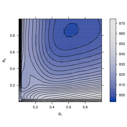
(d)  

Figure 1: The plots show deviance (3) w.r.t. the GP parameter(s) $\theta$. Panels (a) and (b) correspond to Example 1 (with $d=1,n=10$), and (c) and (d) display deviance for Example 2 (with $d=2,n=30$). Panels (b) and (d) are enlargements of (a) and (b) near 0, respectively.

Figure 1 shows that the deviance function is bumpy near $\theta=0$ and there are multiple local optima. Evolutionary algorithms like GA (used by ranjanNugget) are often robust for such objective functions, however, they can be computationally intensive (especially, because the computational cost of $|R|$ and $R^{-1}$ is $O(n^{3})$ and evolutionary algorithms often employ many evaluations of the objective function). Gradient-based optimization might be faster but will require careful selection of initial values to achieve the global minimum of the deviance function. It may be tempting to use a space-filling design over the parameter space for the stating points, however, such designs (e.g., maximin LHD) often tend to stay away from the boundaries and corners. This is unfavourable because the deviance functions (Figure 1) are very active near $\theta=0$.

To address the issue of a bumpy deviance surface near the boundaries of the parameter space, we propose a new parameterization of $R$. Let $\beta_{k}=\log_{10}(\theta_{k})$ for $k=1,...,d$, then

$$R_{ij}=\prod_{k=1}^{d}\exp\left\{-10^{\beta_{k}}|x_{ik}-x_{jk}|^{2}\right\},\qquad\textrm{for all}\quad i,j,$$ (4)

where a small value of $\beta_{k}$ implies a very high spatial correlation or a relatively flat surface in the $k$-th coordinate, and the large values of $\beta_{k}$ imply low correlation, or a very wiggly surface with respect to the $k$-th input factor. Figure 2 displays the two deviance surfaces (shown in Figure 1) under the $\beta$ - parameterization of $R$ (4). Though the new parameterization of $R$ (4) results in an unbounded parameter space $\Omega=(-\infty,\infty)^{d}$, the peaks and dips of the deviance surface are now in the middle of the search space. This should facilitate a thorough search through the local optima and the choice of a set of initial values for a gradient based search.

(a)  

(b)  

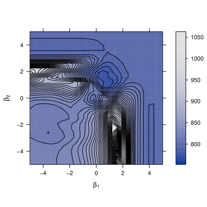
(c)  

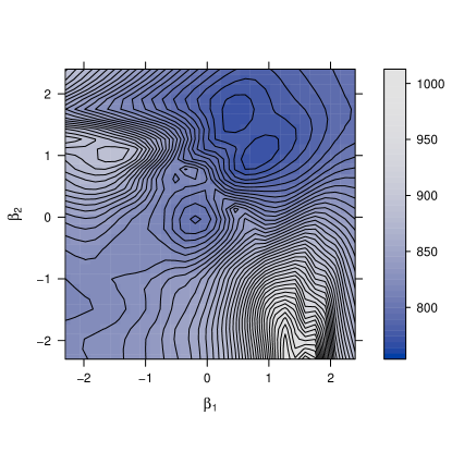
(d)  

Figure 2: The plots show deviance under $\beta$ parameterization of $R$ (4), for the same examples and data as in Figure 1. Panels (a) and (b) correspond to Example 1 (with $d=1,n=10$), and (c) and (d) display deviance for Example 2 (with $d=2,n=30$). Panels (b) and (d) are enlargements of (a) and (b) near 0, respectively.

GPfit uses a multi-start gradient based search algorithm for minimizing the deviance. The gradient based approach is often computationally fast, and careful selection of the multiple initial values of the search algorithm makes our implementation robust.

2.3 Optimization algorithm

A standard gradient based search algorithm like L-BFGS-B (byrd) finds the local optimum closest to the initial value, and thus often gets stuck in the wrong local optima. Our objective is to find $\beta$ that minimizes the deviance function. lawrence argue that a slightly suboptimal solution of the deviance optimization problem may not always be a threat in the GP model setup, as alternative interpretations can be used to justify the model fit. However, the prediction accuracy at unsampled locations may suffer from suboptimal parameter estimates. In an attempt to obtain a good fit of the GP model, GPfit uses a multi-start L-BFGS-B algorithm for optimizing the deviance $-2\log(L_{\beta})$. We first find a subregion $\Omega_{0}$ of the parameter space $\Omega=(-\infty,\infty)^{d}$ that is likely to contain the optimal parameter values. Then, a set of initial values for L-BFGS-B is carefully chosen to cover $\Omega_{0}$.

The structural form of the spatial correlation function (4) guarantees that its value lies in $[0,1]$. That is, excluding the extreme cases of perfectly correlated and absolutely uncorrelated observations, $R_{ij}$ can be approximately bounded as:

$$\exp\{-5\}=0.0067\leq R_{ij}\leq 0.9999=\exp\{-10^{-4}\},$$

or equivalently,

$$10^{-4}\leq\sum_{k=1}^{d}10^{\beta_{k}}|x_{ik}-x_{jk}|^{2}\leq 5.$$

To convert the bounds above into workable ranges for the $\beta_{k}$, we need to consider ranges for $|x_{ik}-x_{jk}|$. Assuming the objective is to approximate the overall simulator surface in $[0,1]^{d}$, loeppky argue that $n=10\cdot d$ is a good rule of thumb for determining the size of a space-filling design over the input locations of the simulator. In this case, the maximum value of the minimum inter-point distance along $k$-th coordinate is $|x_{ik}-x_{jk}|\approx 1/10$. Furthermore, if we also make a simplifying assumption that the simulator is equally smooth in all directions, i.e., $\beta_{k}=\beta_{0}$, then the inequality simplifies to

$$-2-\log_{10}(d)\leq\beta_{k}\leq\log_{10}(500)-\log_{10}(d).$$ (5)

That is, $\Omega_{0}=\{(\beta_{1},...,\beta_{d})\ :\ -2-\log_{10}(d)\leq\beta_{k}\leq\log_{10}(500)-\log_{10}(d),k=1,...,d\}$ is the set of $\beta=(\beta_{1},...,\beta_{d})$ values that is likely to contain the likelihood optimizer. We use $\Omega_{0}$ for restricting the initial values of L-BFGS-B algorithm to a manageable area, and the optimal solutions can be found outside this range.

The initial values for L-BFGS-B can be chosen using a large space-filling LHD on $\Omega_{0}$. However, Figure 2 shows that some parts of the likelihood surface are roughly flat, and multiple starts of L-BFGS-B in such regions might be unnecessary. We use a combination of k-means clustering applied to the design of parameter values, and evaluation of the deviance to reduce a large LHD to a more manageable set of initial values. Since the construction of $\Omega_{0}$ assumed the simplification $\beta_{k}=\beta_{0}$ for all $k$, and in some cases, for instance, in Figure 2(d), the deviance surface appears symmetric in the two coordinates, we enforce the inclusion of an additional initial value of L-BFGS-B on the main diagonal of $\Omega_{0}$. This diagonal point is the best of three L-BFGS-B runs only along the main diagonal, $\beta_{k}=\beta_{0}$ for all $k$.

The deviance optimization algorithm is summarized as follows:

1. Choose a 200$d$-point maximin LHD for $\beta=(\beta_{1},...,\beta_{d})$ in the hyper-rectangle $\Omega_{0}$.

2. Choose the $80d$ values of $\beta$ that correspond to the smallest $-2\log(L_{\beta})$ values.

3. Use k-means clustering algorithm on these $80d$ points to find $2d$ groups. To improve the quality of the clusters, five random restarts of k-means are used.

4. For $d\geq 2$, run L-BFGS-B algorithm along the main diagonal of $\Omega_{0}$ starting at three equidistant points on the diagonal (i.e., at 25%, 50% and 75%). Choose the best of the three L-BFGS-B outputs, i.e., with smallest $-2\log(L_{\beta})$ value.

5. These $2d+1$ (or 2 if $d=1$) initial values, found in Steps 3 and 4, are then used in the L-BFGS-B routine to find the smallest $-2\log(L_{\beta})$ and corresponding $\hat{\beta}_{mle}\in\Omega$.

The multi-start L-BFGS-B algorithm outlined above requires $\left(200d+\sum_{i=1}^{2d+1}\eta_{i}+\sum_{j=1}^{3}\eta_{j}^{\prime}\right)$ deviance evaluations, where $\eta_{i}$ is the number of deviance evaluations for the $i$-th L-BFGS-B run in $\Omega$ space, and $\eta_{j}^{\prime}$ is the number of deviance evaluations for the $j$-th L-BFGS-B run along the diagonal of the $\Omega_{0}$ space. For every iteration of L-BFGS-B, the algorithm computes one gradient (i.e., $2d$ deviance evaluations) and adaptively finds the location of the next step. That is, $\eta_{i}$ and $\eta_{j}^{\prime}$ may vary, and the total number of deviance evaluations in the optimization process cannot be determined. Nonetheless, the empirical evidence based on the examples in Sections 4 and LABEL:sec:mlegp_comp suggest that the optimization algorithm used here is much faster than the GA in ranjanNugget which uses $1000d^{2}$ evaluations of (3) for fitting the GP model in $d$-dimensional input space. Both deviance minimization approaches have a few tunable parameters, for instance, the initial values and the maximum number of iterations (maxit) in L-BFGS-B, and the population size and number of generations in a GA, that can perhaps be adjusted to get better performance (i.e., fewer deviance calls to achieve the same accuracy in optimizing the deviance surface).

3 GPfit package

In this section, we discuss different functions of GPfit that implements our proposed model, which is the computationally stable version of the GP model proposed by ranjanNugget with the new parameterization of correlation matrix $R$ (Section 2.2), and optimization algorithm described in Section 2.3.

The main functions for the users of GPfit are GP_fit(), predict() and (for $d\leq 2$) plot(). Both predict() and plot() use GP_fit()class objects for providing prediction and plots respectively. The code for fitting the GP model to $n$ data points in $d$-dimensional input space stored in an $n\times d$ matrix X and an $n-$ vector Y is: GP_fit(X, Y, control=c(200*d,80*d,2*d), nug_thres=20, trace=FALSE, maxit=100)

The default values of ‘control’, ‘nug_thres’, ‘trace’ and ‘maxit’ worked smoothly for all the examples implemented in this paper, however, they can be changed if necessary.

• control: A vector of three tunable parameters used in the deviance optimization algorithm. The default values correspond to choosing 2*d clusters (using k-means clustering algorithm) based on 80*d best points (smallest deviance) from a 200*d - point random maximin LHD in $\Omega_{0}$.

• nug_thres: A threshold parameter used in the calculation of the lower bound of the nugget, $\delta_{lb}$. Although ranjanNugget suggest nug_thres=25 for space-filling designs, we use a conservative default value nug_thres=20. This value might change for different design schemes.

• trace: A flag that indicates whether or not to print the information on the final runs of the L-BFGS-B algorithm. The default trace=FALSE implies no printing.

• maxit: is the maximum number of iterations per L-BFGS-B run in the deviance optimization. We use the optim package default ‘maxit=100’.

GP_fit() returns the object of class GP that contains the data set X, Y and the estimated model parameters $\hat{\beta},\hat{\sigma}^{2}$ and $\delta_{lb}(\hat{\beta})$. Assuming GPmodel is the GP class object, print(GPmodel,...) presents the values of the object GPmodel, and options like digits can be used for “…". As an alternative, one can use summary(GPmodel) to get the same output.

If xnew contains the set of unobserved inputs, ‘predict(GPmodel, xnew)’ returns the predicted response $\hat{y}(x^{*})$ and the associated MSE $s^{2}(x^{*})$ for every input $x^{*}$ in xnew. It also returns a data frame with the predictions combined with the xnew. The expressions of $\hat{y}(x^{*})$ and $s^{2}(x^{*})$ are shown in Section 2.1 subject to the replacement of $R$ with $R_{\delta_{lb}(\hat{\beta}_{mle})}=R+\delta_{lb}(\hat{\beta}_{mle})I$. The default value of xnew is the design matrix X used for model fitting.

The plotting function plot() takes the GP object as input and depicts the model predictions and the associated MSEs over a regular grid of the $d$-dimensional input space for $d=1$ and $2$. Various graphical options can be specified as additional arguments: plot(GPmodel, range=c(0, 1), resolution=50, colors=c(’black’, ’blue’, ’red’), line_type=c(1, 1), pch=1, cex=2, surf_check=FALSE, response=TRUE, …)

For $d=1$, plot() generates the predicted response $\hat{y}(x)$ and uncertainty bounds $\hat{y}(x)\pm 2s(x)$ over a regular grid of ‘resolution’ many points in the specified range=c(0, 1). The graphical arguments colors, line_type, pch and cex are only applicable for one-dimensional plots. One can also provide additional graphical argument in “…" for changing the plots (see ‘par’ in the base R function ‘plot()’).

For $d=2$, the default arguments of plot() with GP object produces a level plot of $\hat{y}(x^{*})$. The plots are based on the model prediction using predict() at a resolution $\times$ resolution regular grid over $[0,1]^{2}$. The argument surf_check=TRUE can be used to generate a surface plot instead, and MSEs can be plotted by using response=FALSE. Options like shade and drape from wireframe() function, contour and cuts from levelplot() function in lattice (lattice), and color specific arguments in colorspace (seq_hcl; colorspace) can also be passed in for “…".

4 Examples using GPfit

This section demonstrates the usage of GPfit functions and the interpretation of the outputs of the main functions. Two test functions are used as computer simulators to illustrate the functions of this package.

Example 1 Let $x\in[0,1]$, and the computer simulator output, $y(x)$, be generated using the simple one-dimensional test function

$$y(x)=\log(x+0.1)+\sin(5\pi x),$$

referred to as the function computer_simulator below. Suppose we wish to fit the GP model to a data set collected over a random maximin LHD of size $n=7$. The design can be generated using the maximinLHS function in the R package lhs (lhs; stein1987). The following R code shows how to load the packages, generate the simulator outputs and then fit the GP model using GP_fit(). R> library("GPfit") R> library("lhs") R> n = 7 R> x = maximinLHS(n,1) R> y = matrix(0,n,1) R> for(i in 1:n) y[i] = computer_simulator(x[i]) R> GPmodel = GP_fit(x,y) The proposed optimization algorithm used only 227 deviance evaluations for fitting this GP model. The parameter estimates of the fitted GP model are obtained using print(GPmodel). For printing only four significant decimal places, digits=4 can be used in print(). Number Of Observations: n = 7 Input Dimensions: d = 1

Correlation: Exponential (power = 2) Correlation Parameters: beta_hat [1] 1.977

sigma^2_hat: [1] 0.7444 delta_lb(beta_hat): [1] 0 nugget threshold parameter: 20

The GPmodel object can be used to predict and then plot the simulator outputs at a grid of inputs using ‘plot(GPmodel,...)’. Figures 3 and 4 show the model prediction along with the uncertainty bounds $\hat{y}(x^{*})\pm 2s(x^{*})$ on the uniform grid with ‘resolution=100’. Figure 3 compares the predicted and the true simulator output. Figure 4 illustrates the usage of the graphical arguments of plot(). ‘predict(GPmodel,xnew)’ can also be used to obtain model predictions at an arbitrary set of inputs, xnew, in the design space (i.e., not a grid).

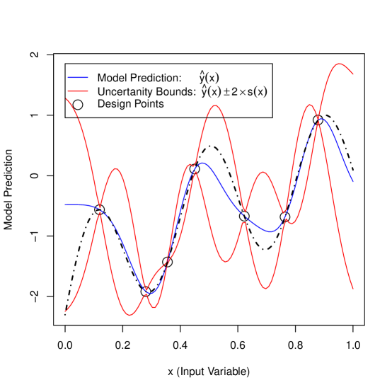
Figure 3: The plot shows the model predictions and uncertainty bands for Example 1. The true simulator output curve is also displayed by the dash-dotted line.

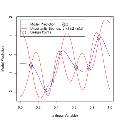
(a) Default arguments

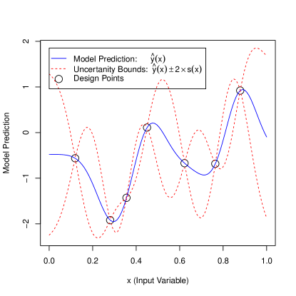
(b) line_type=c(1,2)

(c) cex=3

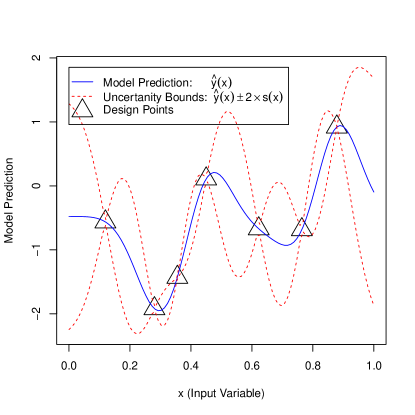
(d) line_type=c(1,2), pch=2, cex=3

Figure 4: The plots illustrate the usage of graphical parameters in plot() for Example 1. Panel (a) shows the model prediction and uncertainty plot with default graphical parameters, (b) illustrates the change due to line_type, (c) highlights the point size using cex, and (d) shows the usage of pch in changing the point character.

Example 2 We now consider a two-dimensional test function to illustrate different functions of GPfit package. Let $x=(x_{1},x_{2})\in[-2,2]^{2}$, and the simulator outputs be generated from the GoldPrice function (andre)

$$y(x) =\left[1+\left({x_{1}}+{x_{2}}+1\right)^{2}\left\{19-{14x_{1}}+3x_{1}^{2}-14x_{2}+6x_{1}x_{2}+3x_{2}^{2}\right\}\right]*$$

$$\left[30+\left(2x_{1}-3x_{2}\right)^{2}(18-32x_{1}+12x_{1}^{2}+48x_{2}-36x_{1}x_{2}+27x_{2}^{2})\right].$$

For convenience the inputs are scaled to $[0,1]^{2}$. The GP_fit() output from fitting the GP model to a data set based on a $20$-point maximin LHD is as follows: Number Of Observations: n = 20 Input Dimensions: d = 2

Correlation: Exponential (power = 2) Correlation Parameters: beta_hat.1 beta_hat.2 [1] 0.8578 1.442

sigma^2_hat: [1] 4.52e+09 delta_lb(beta_hat): [1] 0 nugget threshold parameter: 20

For fitting this GP model, the proposed multi-start L-BFGS-B optimization procedure used only 808 deviance evaluations, whereas the GA based optimization in ranjanNugget would have required $4000$ deviance calls. The correlation hyper-parameter estimate $\hat{\beta}_{mle}=(0.8578,1.442)$ shows that the fitted simulator is slightly more active (or wiggly) in the $X_{2}$ variable. The nugget parameter $\delta_{lb}(\hat{\beta}_{mle})=0$ implies that the correlation matrix with the chosen design points and $\beta=\hat{\beta}_{mle}$ is well-behaved.

The following code illustrates the usage of predict() for obtaining predicted response and associated MSEs at a set of unobserved inputs. R> xnew = matrix(runif(20),ncol=2) R> Model_pred = predict(GPmodel,xnew) The model prediction outputs stored in predict object Model_pred are as follows: $Y_{h}at[1]561.3877-372.522113287.04953148.59045129.1136[6]8188.28053626.498514925.81422869.6225217039.3229\par$MSE [1] 186119713 21523832 86391757 8022989 562589770 [6] 13698589 123121468 1167409027 1483924477 264176788

$complete_{d}ataxnew.1xnew.2Y_{h}atMSE[1,]0.20021450.2732849561.3877186119713[2,]0.68521860.4905132-372.522121523832[3,]0.91687580.318404013287.049586391757[4,]0.28439950.55917283148.59048022989[5,]0.10465010.26259315129.1136562589770[6,]0.70105750.20187528188.280513698589[7,]0.52796000.38752573626.4985123121468[8,]0.80793520.887869814925.81421167409027[9,]0.95650010.55492262869.62251483924477[10,]0.11045300.8421794217039.3229264176788\par The\pkg{GPfit}function\verb"plot()"calls\verb"predict()"forcomputing$^y(x^*)$and$s^2(x^*)$ataregular\verb"`resolution x resolution'"gridintheinputspacedefinedbythe\verb"`range'"parameter.RecallfromSection~{}\ref{sec:gpfit}that\verb"colors",\verb"line_type",\verb"pch"and\verb"cex"areonlyapplicableforonedimensionalplots.For$d=2$,thefollowingcodecanbeusedtodrawthelevel/contourandsurfaceplotsof$^y(x)$and$s^2(x)$overaspecifiedgridresolution.\CodeChunk\CodeInput plot(GPmodel,range=c(0,1),resolution=50,surf_{c}heck=FALSE,response=TRUE,...)\par Additionalgraphicalarguments,forinstance,from\pkg{lattice}and\pkg{colorspace},canalsobepassedinfor``..."toenhancetheplottingfeatures.Figure~{}\ref{fig:eg2}showsthemodelpredictionsandtheMSEsontheuniform$50 ×50$grid.Figures~{}\ref{fig:eg2a}and\ref{fig:eg2b}usedadditionalargument\code{`col.regions=sequential\_hcl(51,power=2.2)^{\prime}}(from\pkg{colorspace}package)tochangethedefaultcolorpalettes.DifferentpanelsofFigure~{}\ref{fig:eg2}highlighttheusageof\code{surf\_check}and\code{response}forobtainingalevelplotandsurfaceplotof$^y(x)$and$s^2(x)$.\text{Figure 5Figure 55Figure 5(a)5(a)5(a)(a)Defaultarguments(a)Defaultarguments(b)5(b)5(b)(b)code}$