Abstract

We study the statistics of the first passage of a random walker to absorbing subsets of the boundary of compact domains in different spatial dimensions. We describe a novel diagnostic method to quantify the trajectory-to-trajectory fluctuations of the first passage, based on the distribution of the so-called uniformity index $\omega$, measuring the similarity of the first passage times of two independent walkers starting at the same location. We show that the characteristic shape of $P(\omega)$ exhibits a transition from unimodal to bimodal, depending on the starting point of the trajectories. From the study of different geometries in one, two and three dimensions, we conclude that this transition is a generic property of first passage phenomena in bounded domains. Our results show that, in general, the Mean First Passage Time (MFPT) is a meaningful characteristic measure of the first passage behaviour only when the Brownian walkers start sufficiently far from the absorbing boundary. Strikingly, in the opposite case, the first passage statistics exhibit large trajectory-to-trajectory fluctuations and the MFPT is not representative of the actual behaviour.

Chapter 0 Trajectory-to-trajectory fluctuations in first-passage phenomena in bounded domains

1 Introduction

The concept of first passage underlies diverse stochastic phenomena for which the crucial aspect is an event when some random variable of interest reaches a preset value for the first time. A few stray examples across disciplines include chemical reactions [1, 2, 3, 4, 5, 6], the firing of a neuron [7, 8], random search of a mobile or an immobile target [9, 10, 11, 12, 13, 14, 15, 16, 17, 18, 19, 20, 21, 22, 23, 24, 25, 26, 27, 28], diffusional disease spreading [29], DNA bubble breathing [30, 31], dynamics of molecular motors [32, 33, 34], the triggering of a stock option [35], etc. One distinguishes also between continuously varying variables for which the first passage across a given preset value coincides with the first arrival to exactly this value, and discontinuous processes for which this value can be overshoot, as it happens, e.g., for Lévy flights characterised by long-tailed jump length distributions with diverging variance [36, 37]. A variety of first passage time phenomena and different related results have been presented in Refs. 38, 39. This volume presents an even broader exposition of relevant areas and describes the state of the art in physical and mathematical comprehension of such phenomena.

In this chapter we will be concerned with first passage phenomena for particles executing Brownian motion. The distribution of first passage times for such processes occurring in unbounded domains is typically broad, such that not even the mean first passage time exists [39]. In particular, in one-dimensional, semi-infinite domains the first passage time distribution of a Markovian process is universally dominated by the $t^{-3/2}$ scaling nailed down by the Sparre Andersen theorem [39]. A similar divergence of the mean first passage time occurs in stochastic processes characterised by scale-free distributions of waiting times [40, 41]. This signifies that sample-to-sample or trajectory-to-trajectory fluctuations are of a crucial importance for such processes so that the mean values — the mean first passage times, even if they exist — have little physical meaning.

However, in many practically important situations first passage processes involve Brownian particles moving in bounded domains (see, e.g., Refs. 42, 43, 44, 45, 46, 47). In this case the random variable of interest, e.g., the first passage time $\tau$ to a boundary, a target chemical group, a binding site on the surface of the domain or elsewhere within the domain, etc., has a distribution $\Psi(\tau)$ which possesses moments of arbitrary, negative and positive order. Such distributions are usually considered narrow, as opposed to broad distributions, which do not possess all moments [38, 39, 40, 41, 36, 37].

Nonetheless, even for such distributions first passage variables do fluctuate, of course, from sample to sample or from trajectory to trajectory, and an important question is how to quantify such fluctuations. One usually resorts to standard measures of the statistical analysis, such as, e.g., standard deviations, the skewness or the kurtosis of the distribution. But these quantities are often not very instructive since they just produce numbers and it is not always evident how to interpret or compare them. Clearly, quantifying the trajectory-to-trajectory fluctuations in a robust and meaningful way is a challenging problem with many important applications.

In this chapter we focus on this non-trivial problem and discuss a recently proposed procedure which presents a lucid illustration of the effect of the trajectory-to-trajectory fluctuations. It allows to quantify their impact and, moreover, shows that in some cases the distributions considered as narrow behave effectively as broad distributions [22, 23]. We employ a novel diagnostic method based on the concept of simultaneity of first passage events. Instead of the original first passage problem of quantifying the statistical outcome for a single Brownian walker, in this procedure one simultaneously launches two identical, independent Brownian particles at the same position ${\bf r_{0}}$, namely two different realisations of a single Brownian Motion (BM) starting at ${\bf r_{0}}$. The corresponding outcomes are the first passage times $\tau_{1}$ and $\tau_{2}$. One defines then the random variable

$$\omega\equiv\frac{\tau_{1}}{\tau_{1}+\tau_{2}},$$ (1)

such that $\omega$ ranges in the interval $[0,1]$. The uniformity index $\omega$ measures the likelihood that both walkers arrive to the target simultaneously: when $\omega$ is close to 1/2, the process is uniform and the particles behave as if they were almost performing a Prussian Gleichschritt. In contrast, values of $\omega$ close to 0 or 1 mean highly non-uniform behaviour, strongly affecting the trajectory-to-trajectory fluctuations. We note parenthetically that similar random variables have been used in the analysis of random probabilities induced by normalisation of self-similar Lévy processes [48], of the fractal characterisation of Paretian Poisson processes [49], and of the so-called Matchmaking paradox [50, 51], and more recently, to quantify sample-to-sample fluctuations in mathematical finances [52, 53], chaotic systems [54], the analysis of distributions of the diffusion coefficient of proteins diffusing along DNAs[55] and optimal estimators of the diffusion coefficient of a single Brownian trajectory.[56]

To illustrate the concept of simultaneity, consider a generic, generalized inverse Gaussian form of $\Psi(\tau)$ (see e.g., the discussion in Ref. 22, 23 and references therein)

$$\Psi(\tau)\sim\exp\left(-\frac{a}{\tau}\right)\frac{1}{\tau^{1+\mu}}\exp\left(-\frac{\tau}{b}\right),$$ (2)

where $a$ and $b$ are some constants. Note that the first passage time distribution in Eq. (2) is exact in the particular case of Brownian motion on a semi-infinite line in presence of a bias pointing towards the target site, or, equivalently, for the celebrated integrate-and-fire model of neuron firing by Gerstein and Mandelbrot [7]. In general, the detailed form of $\Psi(\tau)$ for diffusion in bounded domains is obviously much more complex than given by Eq. (2), depending on the shape of the domain under consideration and the exact boundary value problem and is typically given in terms of an infinite series.

Nonetheless, on a qualitative level eq:Pt-exptrunc provides a clear picture of the actual behaviour of the first passage time distribution in bounded domains. Namely, $\Psi(\tau)$ consists of three different parts: a singular decay for small values of $\tau$, which mirrors the fact that the first passage to some point starting from a distant position cannot occur instantaneously. This is followed at intermediate times by a generic power-law decay with exponent $\mu$ — the so-called persistence exponent [57, 58], depending on the exact type of random motion and spatial dimension. Finally, an exponential decay at long $\tau$ cuts off the power-law. A crucial aspect is that the exponential cutoffs at both short and long $\tau$ ensure that in bounded domains $\Psi(\tau)$ possesses moments of arbitrary positive or negative order. The parameters $a$ and $b$ depend on the shape of the domain, its typical size, and the starting position of the particle within the domain. When the linear size of the domain (say, the radius $R$ of a circular or a spherical domain) diverges (i.e., $R\to\infty$), the parameter $b$ also diverges such that the long-time asymptotic behaviour of the first passage time distribution is of power-law form without a cutoff. In this case, at least some, if not all, of the moments of $\Psi(\tau)$ diverge.

Now, given the distribution $\Psi(\tau)$, the distribution of the uniformity index $\omega$ in Eq. (1) can be readily calculated to give [53, 54]

$$P(\omega)=\frac{1}{(1-\omega)^{2}}\int^{\infty}_{0}\tau d\tau\Psi(\tau)\Psi\left(\frac{\omega}{1-\omega}\tau\right)\,.$$ (3)

As we explicitly show in the following section 2, for the generic distribution in Eq. (2) one finds the following explicit form [23]:

$$P(\omega)=\frac{1}{2K_{\mu}^{2}\left(2\sqrt{a/b}\right)}\frac{1}{\omega(1-\omega)}K_{2\mu}\left(2\sqrt{\frac{a}{b\omega(1-\omega)}}\right)\,,$$ (4)

where $K_{2\mu}(\cdot)$ is the modified Bessel function of the second type.

One notices first that the form of the distribution $P(\omega)$ in Eq. (4) is distinctly sensitive to the value of the persistence exponent $\mu$, which characterises the scaling behaviour of the first passage time distribution $\Psi(\tau)$ at intermediate times. Thus, for $\mu>1$, $P(\omega)$ is always a unimodal, bell-shaped function with a maximum at $\omega=1/2$, which implies that in such a situation both walkers (or two distinct trajectories of one walker) will most likely arrive to the target simultaneously. For $\mu=1$, $P(\omega)$ is almost uniform, $P(\omega)\approx 1$, apart from narrow regions at the corners $\omega=0$ and $\omega=1$, for $b/a\gg 1$. Curiously, for $\mu<1$, which corresponds to the most common case, there exists a critical value $p_{c}$ of the ratio $p=b/a$ such that for $p>p_{c}$ the distribution $P(\omega)$ has a characteristic M-shaped form with two maxima close to 0 and 1, while at $\omega=1/2$ one finds a local minimum. Such a transition from a unimodal, bell-shaped to bimodal, M-shaped form mirrors a significant manifestation of sample-to-sample fluctuations.

In what follows we survey known results and further explore this intriguing behaviour of the first passage time distribution and of the corresponding distribution of the uniformity index $\omega$ for diffusion in bounded domains, focusing on the effects of the domain shape, dimensionality, location of the target, the type of the boundary conditions, and of the initial position of the walker.

2 First Passage Times and the Uniformity Distribution

Consider a BM inside a general $d$-dimensional domain $\mathcal{S}$, whose boundary $\partial\mathcal{S}\equiv\partial\mathcal{S}_{a}\cup\partial\mathcal{S}_{r}$ comprises reflecting, $\partial\mathcal{S}_{r}$, and absorbing, $\partial\mathcal{S}_{a}$, parts. At time $t=0$, the BM initiates at $\mathbf{r}_{0}\in\mathcal{S}$ and evolves within the domain until the trajectory hits $\partial\mathcal{S}_{a}$ for the first time at some random instant $\tau$. Furthermore, let $P(\mathbf{r},t|\mathbf{r}_{0})$ denote the conditional probability distribution for finding the Brownian walker at position $\mathbf{r}$ at time $t$, provided the initial condition was at $\mathbf{r}_{0}$ at $t=0$. The distribution $P(\mathbf{r},t|\mathbf{r}_{0})$ is the solution of the diffusion equation

$${\partial_{t}}P(\mathbf{r},t|\mathbf{r}_{0})=D~{}\partial^{2}_{\mathbf{r}}P(\mathbf{r},t|\mathbf{r}_{0})$$ (5)

on $\mathcal{S}$, subject to the initial condition as well as the boundary conditions at $\partial\mathcal{S}$. Here $D$ is the diffusion coefficient and $\partial^{2}_{\mathbf{r}}$ is the $d$-dimensional Laplacian. The solution of this initial boundary value problem is, in the best case, cumbersome, and explicit solutions may be obtained for only few simple geometries, (see e.g.Ref. 59).

If a finite part of the boundary is absorbing, i.e., $\partial\mathcal{S}_{a}$ is not empty, then the distribution $P(\mathbf{r},t|\mathbf{r}_{0})$ is no longer normalised. The survival probability $\mathscr{S}_{\mathbf{r}_{0}}(t)$ that the walker has not reached $\partial\mathcal{S}_{a}$ up to time $t$, is defined by

$$\mathscr{S}_{\mathbf{r}_{0}}(t)=\int_{\mathcal{S}}P(\mathbf{r},t|\mathbf{r}_{0})d\mathbf{r}.$$ (6)

$\mathscr{S}_{\mathbf{r}_{0}}(t)$ is a monotonically decreasing function of time, eventually reaching zero value, $\lim_{t\to\infty}\mathscr{S}_{\mathbf{r}_{0}}(t)=0$. In terms of the survival probability, the distribution of first passage times to the absorbing boundary becomes

$$\Psi_{\mathbf{r}_{0}}(\tau)=-\frac{d\mathscr{S}_{\mathbf{r}_{0}}(\tau)}{d\tau}\ ,$$ (7)

and the MFPT associated with the distribution $\Psi(\tau)$ is defined as the first moment

$$\langle\tau\rangle(\mathbf{r}_{0})=\int_{0}^{\infty}\tau\Psi_{\mathbf{r}_{0}}(\tau)d\tau=\int_{0}^{\infty}\mathscr{S}_{\mathbf{r}_{0}}(\tau)d\tau.$$ (8)

In most of the existing literature, the dependence of the MFPT on the starting position of the walker is either simply neglected, or it is assumed that the starting point is randomly distributed within the domain $\mathcal{S}$. However, as we proceed to show, the $\mathbf{r}_{0}$-dependence of the first passage time distribution is a crucial aspect which cannot be neglected.

From the First Passage Time Distribution (FPTD) one readily obtains the distribution of the uniformity index $\omega$ defined in def:omega, for two independent BM, in terms of its moment generating function

$$\Phi(\lambda)=\int_{0}^{1}P(\omega)\exp\left(-\lambda\omega\right)d\omega,$$ (9)

with $\lambda\geq 0$. Since $\tau_{1}$ and $\tau_{2}$ are independent, identically distributed random variables, expression (9) can be formally represented as

$$\Phi(\lambda)=\int^{\infty}_{0}\int^{\infty}_{0}\Psi(\tau_{1})\Psi(\tau_{2})\exp\left(-\lambda\frac{\tau_{1}}{\tau_{1}+\tau_{2}}\right)d\tau_{1}d\tau_{2}.$$ (10)

Integrating over $d\tau_{1}$ we change the integration variable, $\tau_{1}\to\omega$, so that Eq. (10) is rewritten in the form

$$\Phi(\lambda)=\int^{1}_{0}\exp\left(-\lambda\omega\right)\frac{d\omega}{(1-\omega)^{2}}\int^{\infty}_{0}\tau_{2}\Psi(\tau_{2})\Psi\left(\frac{\omega}{1-\omega}\tau_{2}\right)d\tau_{2}.$$ (11)

From comparison with Eq. (9), one obtains $P(\omega)$ in def:Pw.

1 Trajectory-to-trajectory fluctuations and the shape of $P(\omega)$

To better grasp the relation between the trajectory-to-trajectory fluctuations and the distribution of the uniformity index, consider $P(\omega)$ of eq:Pw-exptrunc corresponding to the FPTD of eq:Pt-exptrunc. First, one readily notices that $P(\omega)$ vanishes exponentially fast when $\omega\to 0$ or $\omega\to 1$ so that $P(\omega=0)=P(\omega=1)=0$. Second, $P(\omega)$ is symmetric under the replacement $\omega\to 1-\omega$. Since the distribution $\Psi(\tau)$ possesses moments of arbitrary order, our first guess would be that $P(\omega)$ is always a bell-shaped function with a maximum at $\omega=1/2$.

To study the shape of the distribution of the uniformity index, we expand $P(\omega)$ in Taylor series around its symmetric point $\omega=1/2$ up to second order in $\left(\omega-\frac{1}{2}\right)^{4}$,

$$P(\omega)\approx\frac{2K_{2\mu}(2C)}{K^{2}_{\mu}(C)}\,\Bigg{[}1+4\left(1-\mu-C\frac{K_{2\mu-1}(2C)}{K_{2\mu}(2C)}\right)\left(\omega-\frac{1}{2}\right)^{2}\Bigg{]}\ ,$$ (12)

where $C\equiv 2\sqrt{a/b}$. Inspecting the sign of the coefficient before the quadratic term, i.e.,

$$g=1-\mu-C\frac{K_{2\mu-1}(2C)}{K_{2\mu}(2C)},$$ (13)

we notice that

• For $\mu>1$, $g$ is always negative for any value of $b/a$ so that here the distribution $P(\omega)$ is a bell-shaped function with a maximum at $\omega=1/2$.

• For $\mu=1$, $g$ is negative and approaches $0$ from below when $b/a\to\infty$. It means that $P(\omega)$ is generally a bell-shaped function with a maximum at $\omega=1/2$, but it becomes progressively flatter when $b/a$ is increased, so that ultimately $P(\omega)\approx 1$ apart from very narrow regions at the edges for $b/a\gg 1$.

• For $0\leq\mu<1$ there always exists a critical value $y_{c}(\mu)$ of the parameter $y=b/a$ which is defined implicitly as the solution of g for $g=0$. For $b/a<y_{c}(\mu)$, the distribution $P(\omega)$ is unimodal with a maximum at $\omega=1/2$. For $b/a=y_{c}(\mu)$, the distribution is nearly uniform except for narrow regions in the vicinity of the edges. Finally, which is quite surprising in view of the fact that in this case $\Psi(\tau)$ possesses all moments, for $b/a>y_{c}(\mu)$ the distribution $P(\omega)$ is bimodal with a characteristic M-shaped form, two maxima close to $0$ and $1$ and $\omega=1/2$ being the least probable value.

We depict in Fig. 1 three characteristic forms of $P(\omega)$ for $\mu=1/2$ and three different values of $b/a$.

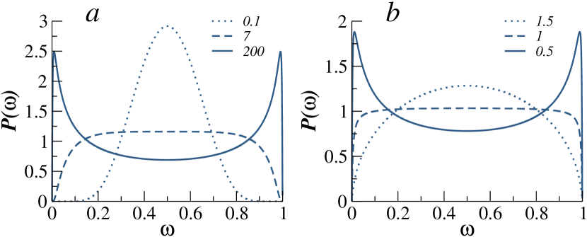
Figure 1: The distribution $P(\omega)$ of eq:Pw-exptrunc: Panel $(a)$, for $\mu=0.25$ and different values of $b$. Panel $(b)$, for $b=200$ and different values of $\mu$. Parameter $a$ is set equal to $1$.

Therefore, for $\mu\geq 1$ two independent BMs will most probably reach the target simultaneously. For $0\leq\mu<1$ two distinctly different situations are possible: if $b/a$ is less than some well-defined critical value $y_{c}(\mu)$, then most likely both BM will arrive to the target for the first time together. If, on the contrary, $b/a$ exceeds this critical value, the event in which both BMs arrive to the location of the target simultaneously will be the least probable one, yielding very large fluctuations in the MFPT obtained from different trajectories.

In the rest of this chapter we present several concrete examples in which the transition between unimodal and bimodal distributions of $P(\omega)$ is observed.

3 One-dimensional Brownian Motions

In this section we study the trajectory-to-trajectory fluctuations of the first passage time, in terms of the distribution of the uniformity index $\omega$ for two independent identical BM.

1 BM in the semi-infinite interval with a bias

We first consider a BM in the semi-infinite interval $\mathcal{S}\equiv[0,\infty)$ with $\partial\mathcal{S}_{a}=\{0\}$ and $\partial\mathcal{S}_{r}=\{\infty\}$, in the presence of a constant bias pointing towards the target, for which the FPTD in eq:Pt-exptrunc with $\mu=1/2$ is exact. In this case one has $a=x_{0}^{2}/4D$, where $x_{0}$ is the starting point, $D$ the diffusion coefficient, and $b=4D/v^{2}$ ($v$ being the drift velocity). Hence, the Péclet number, defined as the ratio between the rate of advection and the rate of diffusion, is $\mathrm{Pe}=2\sqrt{a/b}=x_{0}|v|/2D$ (see, e.g., Ref. 39). Consequently, we can make a following statement:

Consider two independent identical BMs on a semi-infinite interval, starting at the same point $x_{0}$, having the same diffusion coefficient $D$ and experiencing the same bias $F$ which points towards the origin so that the drift velocity of both BMs is $v<0$. Then, an event in which both BMs arrive for the first time to the origin simultaneously is

• the least probable if $\mathrm{Pe}<\mathrm{Pe}_{c}$ ,

• the most probable if $\mathrm{Pe}>\mathrm{Pe}_{c}$ ,

where $\mathrm{Pe}_{c}$ is the solution of the transcendental equation

$$1=2\mathrm{Pe}_{c}\frac{K_{0}(2\mathrm{Pe}_{c})}{K_{1}(2\mathrm{Pe}_{c})}\approx 0.666\ .$$ (14)

Therefore, the MFPT to the target, which in this case equals $x_{0}/|v|$, might be an appropriate measure of the search efficiency for sufficiently large Péclet numbers, but definitely is not in case of small $\mathrm{Pe}$. In the latter case the trajectory-to-trajectory fluctuations are significant and the mean value is not representative of the actual behaviour.

2 BM on a finite interval

We consider now BMs in the finite interval $\mathcal{S}\equiv[0,L]$ with $\partial\mathcal{S}_{a}=\{0\}$ and $\partial\mathcal{S}_{r}=\{L\}$, that are initiated at $x=x_{0}$ at time $t=0$. In this case the FPTD can be obtained exactly as the infinite sum

$$\Psi_{x_{0}}(\tau)=\frac{2\pi D}{L^{2}}\sum_{n=0}^{\infty}A_{n}\left(\frac{x_{0}}{L}\right)\exp\left(-\frac{\pi^{2}(n+1/2)^{2}D\tau}{L^{2}}\right),$$ (15)

where the coefficients $A_{n}\left(\frac{x_{0}}{L}\right)=\left(n+\frac{1}{2}\right)\sin\left(\frac{\pi(n+1/2)x_{0}}{L}\right)$. Consequently, after some calculations the normalised distribution $P(\omega)$ has the following form[22]

$$P(\omega)=\frac{2}{\pi}\frac{d}{d\omega}\sum_{m=0}^{\infty}\frac{\sin\left(\pi(m+1/2)\frac{x_{0}}{L}\right)}{m+1/2}\frac{\cosh\left(\pi(m+1/2)\sqrt{\frac{1-\omega}{\omega}}\left(1-\frac{x_{0}}{L}\right)\right)}{\cosh\left(\pi(m+1/2)\sqrt{\frac{1-\omega}{\omega}}\right)}\,.$$ (16)

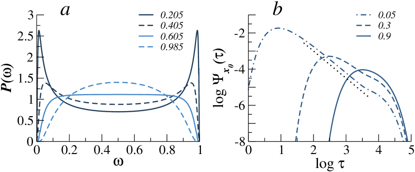
Figure 2: Two BMs in the interval $[0,L]$. Panel $(a)$: Distribution $P(\omega)$ in Eq. (16) for different values of $x_{0}/L$. Panel $(b)$: FPTD $\Psi_{x_{0}}(\tau)$ in Eq. (15) for $L=100$, $D=1/2$ and different values of $x_{0}/L$. The dotted curve corresponds to a decay $\sim\tau^{-3/2}$.

Panel $(a)$ of Fig. 2 shows the distribution $P(\omega)$ in pw1d for different values of the ratio $x_{0}/L$, evidencing the transition in the shape of $P(\omega)$ at the critical value $\approx 0.605$.

Furthermore, the moments of arbitrary order of $\Psi(\tau)$ in Eq. (15) can be straightforwardly calculated. One obtains

$$\big{<}\tau^{m}\big{>}\equiv\int^{\infty}_{0}\tau^{m}\,d\tau\,\Psi(\tau)=\frac{(-1)^{m}\sqrt{\pi}}{\Gamma(m+1/2)}\left(\frac{L^{2}}{D}\right)^{m}E_{2m}\left(\frac{x_{0}}{2L}\right)\,,$$ (17)

where $E_{2k}(\cdot)$ are the Euler polynomials. Consequently, the mean and the variance are given by

$$\big{<}\tau\big{>}=-2\frac{L^{2}}{D}\,E_{2}\left(\frac{x_{0}}{2L}\right),$$ (18)

and

$$k_{2}=\big{<}\tau^{2}\big{>}-\big{<}\tau\big{>}^{2}=\frac{4}{3}\frac{L^{4}}{D^{2}}\left(E_{4}\left(\frac{x_{0}}{2L}\right)-3E_{2}^{2}\left(\frac{x_{0}}{2L}\right)\right)\,$$ (19)

respectively. One can readily check that both statistical measures are monotonically increasing functions of $x_{0}/L$ and do not show any sign of a particular behaviour at $x_{0}/L\approx 0.605$. The same occurs for higher order cumulants of the distribution $\Psi(\tau)$ [22].

This puts in evidence the superior sensitivity of the statistics of the uniformity index $\omega$. As we show in sections 2 and 2 , the unimodal or bimodal shape of $P(\omega)$ classifies the parameter space into regions inside which the MFPT is either meaningful or meaningless.

3 Arcsine law mechanism

We found that any two BMs arrive to the target at progressively distinct times the closer they are initially to its location, and should most probably arrive together when they are far from it. Notwithstanding this counterintuitive result, such a behavior is the same as the one behind the famous arcsine law for the distribution of the fraction of time spent by a random walker on a positive half-axis [60]:

Once one of the BMs goes away from the target, it finds it more difficult to return than to keep on going away.

How does this relate to the properties of the distribution of the first passage time? In terms of the FPTD of fpt1 in the previous section, $x_{0}$ ($a^{1/2}$) and $l$ ($b^{1/2}$) define the effective size of the region in which the decay of the FPTD is governed by the intermediate power-law tail. The larger this region is the larger the fluctuations in the first passage time become[22]. This is shown in panel $(b)$ of Fig. 2. All three curves show an exponential behavior for small and large values of $\tau$, as in eq:Pt-exptrunc. For large $\tau$ all three curves merge which signifies that at such values of $\tau$ the characteristic decay time is dependent only on $l$. The lower cut-off is clearly dependent only on the starting point $x_{0}$. Evidently the power-law region characterized by a decay $\sim t^{-3/2}$, grows with decreasing $x_{0}/l$, i.e., when the BMs start closer to the target.

4 Two-dimensional Brownian Motions

In this section we analyse the statistics of $\omega$ for BM in different two-dimensional bounded domains.

1 BM in a disc with a reflecting boundary

We first consider BM in a disc of radius $L$, centered at the origin $\mathcal{S}=\{\mathbf{r}:|\mathbf{r}|<L\}$, with $\partial\mathcal{S}_{a}=\{\mathbf{r}:|\mathbf{r}|=l\}$ and $\partial\mathcal{S}_{r}=\{\mathbf{r}:|\mathbf{r}|=L\}$, where $\mathbf{r}\in\mathbb{R}^{2}$ and $l<L$. Therefore, the target consist in a concentric disc of smaller radius $l$.

Suppose next that a BM starts at some point at distance $r_{0}$ from the origin and hits the target for the first time at time moment $\tau$. The FPTD $\Psi_{r_{0}}(\tau)$ is explicitly given by [22]

$$\Psi_{r_{0}}(\tau)=\frac{lD}{Z}\sum_{n=0}^{\infty}A_{n}(l,r_{0},L)\exp\left(-\lambda_{n}^{2}D\tau\right),$$ (20)

where $Z$ is the normalization,

$$A_{n}(l,r_{0},L)=\frac{U_{0}(\lambda_{n}r_{0})U_{0}^{\prime}(\lambda_{n}l)}{\lambda_{n}^{2}L^{2}U_{0}^{2}(\lambda_{n}L)-l^{2}\left(U_{0}^{\prime}(\lambda_{n}l)\right)^{2}},$$

$$U_{0}(x)=Y_{0}(\lambda_{n}l)J_{0}(x)-J_{0}(\lambda_{n}l)Y_{0}(x);\quad U_{0}^{\prime}(\lambda_{n}l)=\frac{dU_{0}(\lambda_{n}x)}{dx}\bigg{|}_{x=l}$$

while $\lambda_{n}$ are the roots of the function $Y_{0}(\lambda_{n}l)J_{1}(\lambda_{n}L)-J_{0}(\lambda_{n}l)Y_{1}(\lambda_{n}L)$, arranged in an ascending order, and $Y_{n}(\cdot)$ are Bessel functions of the second kind. Note that $\lambda_{n}$ depends on $L$ and $l$.

In this case the distribution of the uniformity index $\omega$ can be written as [22]

$$P(\omega)=\frac{l}{Z}\frac{d}{d\omega}\sum_{m=0}^{\infty}\frac{A_{m}(l,r_{0},L)}{\lambda_{m}^{2}}\,\Phi\left(\lambda=\frac{1-\omega}{\omega}D\lambda_{m}^{2}\right)\,,$$ (21)

where $\Phi(\lambda)$ is the characteristic function of the first passage time distribution in Eq. (20) defined by [39]

$$\Phi(\lambda)=\frac{I_{0}\left(\sqrt{\frac{\lambda}{D}}r_{0}\right)K_{1}\left(\sqrt{\frac{\lambda}{D}}L\right)+K_{0}\left(\sqrt{\frac{\lambda}{D}}r_{0}\right)I_{1}\left(\sqrt{\frac{\lambda}{D}}L\right)}{I_{0}\left(\sqrt{\frac{\lambda}{D}}l\right)K_{1}\left(\sqrt{\frac{\lambda}{D}}L\right)+K_{0}\left(\sqrt{\frac{\lambda}{D}}l\right)I_{1}\left(\sqrt{\frac{\lambda}{D}}L\right)}\,.$$ (22)

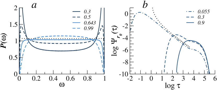
Figure 3: Two BMs in the two-dimensional disc of radius $L=100$ with a reflecting boundary and concentric absorbing disc of radius $l=5$, and $D=1/2$. Panel $(a)$: Distribution $P(\omega)$ in Eq. (21) for different values of $r_{0}/L$. The dotted curve corresponds to $P_{\mathrm{av}}(\omega)$. Panel $(b)$: FPTD $\Psi_{r_{0}}(\tau)$ in Eq. (20) for different values of $r_{0}/L$. The dotted curve corresponds to a decay $\sim 1/\tau\log^{2}\tau$.

Fig. 3 shows the FPTD in Eq. (20) and $P(\omega)$ in Eq. (21) for fixed $L$, $D$ and $r$, and several values of $r_{0}$. Here we observe the same trend as in the previous one-dimensional example, namely the FPTD becomes broader when the starting point of the BMs is closer to $\partial\mathcal{S}_{a}$, with an intermediate power-law behavior with a logarithmic correction $\sim 1/\tau\log^{2}(\tau)$ (see the dashed curve in Fig. 3-$b$). The critical value for the transition between bell- and M-shaped $P(\omega)$ is numerically found to be $r_{0}/L\sim 0.643$. Moreover, if the starting point of two BM is averaged over the domain $\mathcal{S}$, one readily finds, by averaging the result in Eq. (21), that $P_{av}(\omega)\equiv 1$ (see the dashed curve in Fig. 3-$b$).

2 BM in a disc with aperture

For other simple geometries but mixed absorbing/reflecting boundary conditions, it is not possible in general to obtain analytical closed expressions for the FPTD. However, the examples discussed previously suggest that the arcsine law mechanism in section 3, underlying the appearance of large trajectory-to-trajectory fluctuations of the first passage time, is generic in bounded domains of arbitrary shape.

For instance, consider a circular domain of unit radius (in polar coordinates $\mathbf{r}=(r,\theta)$), $\mathcal{S}=\{\mathbf{r}:r<1\}$, and the following boundary conditions: the segment with $|\theta|<\Theta/2$ is absorbing while the remaining part of the outer circle is reflective. The aperture of the circular domain is thus an arc of length $\Theta$.

Obtaining an expression for the FPTD involves the cumbersome problem of finding the solution of the diffusion equation with mixed Dirichlet-Neumann boundary conditions. Here we content ourselves with the numerical analysis of the problem. Let each BM commence at position $(\rho_{0},\theta_{0})$ inside the unit circle and determine the set $\{\tau_{i}\}$ of first passage times to the location of the aperture. From these data one obtains $P(\omega)$. To easily grasp the geometric dependence of the first passage time fluctuations, we considered the parameter $\chi$ that quantifies the shape of the distribution of $\omega$[23]. Performing a fit of the numerically obtained $P(\omega)$ to a quadratic polynomial of $\omega$ in the domain $0.05<\omega<0.95$, we define $\chi$ as the coefficient of the quadratic term, so that the sign of $\chi$ determines the shape of $P(\omega)$: $\chi<0$ corresponds to the unimodal, bell-shaped distribution, $\chi>0$ signifies that the distribution is bimodal, M-shaped, and a zero value of $\chi=0$ means that $P(\omega)$ is uniform.

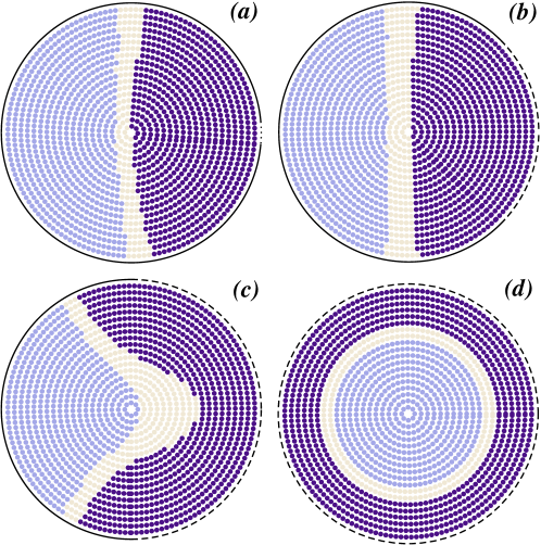
Figure 4: Phase-chart for the shape of the uniformity distribution $P(\omega)$ for a BM in the unit disc with reflective boundary (solid line) and an aperture of size $\Theta$ corresponding to the absorbing boundary (dashed line). (a) $\Theta=\pi/18$, (b) $\Theta=\pi/2$, (c) $\Theta=\pi$, and (d) $\Theta=2\pi$. Starting locations are coloured light blue if $\chi<-\chi_{\star}$, dark blue if $\chi>\chi_{\star}$ and beige if $|\chi|<\chi_{\star}$, where $\chi_{\star}=1$.

In Fig. 4 we show the phase-chart for the shape of $P(\omega)$ for different sizes of the aperture . As in all previous examples, the closer the starting position of the BM is to the absorbing boundary the larger the fluctuations of the first passage time become. One thus expects that very near the absorbing boundary the standard deviation of the first passage time becomes much larger than its mean. We note that this result is generic irrespectively of the aperture size.

The same analysis was recently carried out for other different shapes, such as pie-wedges or triangles in Ref. 23, with the same conclusions.

5 Three-dimensional Brownian Motions

1 BM in a sphere with a reflecting boundary

Consider a BM in a sphere of radius $L$ (in spherical coordinates $\mathbf{r}=(\rho,\theta,\phi)$), $\mathcal{S}=\{\mathbf{r}:\rho<L\}$ with reflecting boundary $\partial\mathcal{S}_{r}=\{\mathbf{r}:\rho=L\}$, and a concentric absorbing sphere of radius $l<L$, $\partial\mathcal{S}_{a}=\{\mathbf{r}:\rho=l\}$.

For this geometry, the distribution of the first passage time $\tau$ of a BM starting at a distance $\rho_{0}$ from the origin to the surface of the target is given explicitly by[22]

$$\Psi_{\rho_{0}}(\tau)=\frac{D}{Z}\sum_{n=0}^{\infty}A_{n}(l,\rho_{0},L)\exp\left(-\lambda_{n}^{2}D\tau\right)\ ,$$ (23)

where the coefficients

$$A_{n}(l,\rho_{0},L)=\frac{2u_{0}(\lambda_{n}\rho_{0})u_{0}^{\prime}(\lambda_{n}l)}{G(l,L,\lambda_{n})}\ ,$$

with $u_{0}(x)=y_{0}(\lambda_{n}l)j_{0}(x)-j_{0}(\lambda_{n}l)y_{0}(x)$, $u_{0}^{\prime}(\lambda_{n}l)=du_{0}(\lambda_{n}x)/dx|_{x=l}$, and

$$G(l,L,\lambda_{n}) = Rj_{0}(\lambda_{n}L)u_{0}(\lambda_{n}L)(\lambda_{n}Lj_{0}(\lambda_{n}l)-y_{0}(\lambda_{n}l))-$$

$$- \frac{j_{0}(\lambda_{n}l)y_{0}(\lambda_{n}l)}{\lambda_{n}}+\frac{L-l}{l^{2}\lambda_{n}^{4}}\ .$$

The set $\{\lambda_{n}\}$ are the roots of $y_{0}(\lambda_{n}l)j_{1}(\lambda_{n}L)-j_{0}(\lambda_{n}l)y_{1}(\lambda_{n}L)$, arranged in an ascending order, while $j_{n}(\cdot)$ and $y_{n}(\cdot)$ are the spherical Bessel functions of the first and of the second kind, respectively.

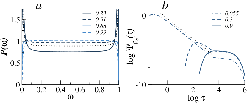
Figure 5: BM in a sphere of radius $L=100$ with a reflecting boundary and concentric absorbing sphere of radius $l=5$, and $D=1/2$. Panel $(a)$: Distribution $P(\omega)$ in Eq. (24) for different values of $\rho_{0}/L$. The dotted curve corresponds to $P_{\mathrm{av}}(\omega)$. Panel $(b)$: FPTD $\Psi_{\rho_{0}}(\tau)$ in Eq. (23) for different values of $\rho_{0}/L$. The dotted curve corresponds to a decay $\tau^{-3/2}$.

The corresponding distribution $P(\omega)$ for two independent BMs starting at a distance $\rho_{0}$ from the origin is [22]

$$P(\omega) = \frac{1}{Z^{2}}\sum_{n,m=0}^{\infty}\frac{A_{n}(l,\rho_{0},L)A_{m}(l,\rho_{0},L)}{\left(\omega\lambda_{n}^{2}+(1-\omega)\lambda_{m}^{2}\right)^{2}}=$$ (24)

$$= \frac{1}{Z}\sum_{m=0}^{\infty}\frac{A_{m}(l,\rho_{0},L)}{\lambda_{m}^{2}}\,\Phi\left(\lambda=\frac{1-\omega}{\omega}D\lambda_{m}^{2}\right)\,,$$

where $\Phi(\lambda)$ is the characteristic function of $\Psi(\tau)$ in Eq. (23), defined by [39]

$$\Phi(\lambda)=\frac{l}{\rho_{0}}\frac{\sinh\left(\sqrt{\frac{\lambda}{D}}\left(L-\rho_{0}\right)\right)-\sqrt{\frac{\lambda}{D}}\,R\,\cosh\left(\sqrt{\frac{\lambda}{D}}\left(L-\rho_{0}\right)\right)}{\sinh\left(\sqrt{\frac{\lambda}{D}}\left(L-l\right)\right)-\sqrt{\frac{\lambda}{D}}\,R\,\cosh\left(\sqrt{\frac{\lambda}{D}}\left(L-l\right)\right)}\,.$$ (25)

The distributions in Eqs. (23) and (24) are shown in Fig. 5 for fixed $L$, $l$ and $D$, and several values of $\rho_{0}$. An intermediate power-law $\sim\tau^{-3/2}$ is apparent for $\rho_{0}/L=0.055$, persists for one decade for $\rho_{0}/L=0.3$ and is entirely absent for $\rho_{0}/L=0.9$, i.e., when the BM initiates close to the reflecting boundary (see Fig. 5-$b$). Correspondingly we find that $P(\omega)$ has a different modality depending on the value of the ratio $\rho_{0}/L$ with a critical value of $\rho_{0}/L\sim 0.68$ (see Fig. 5-$a$). For $\rho_{0}/L>0.68$, the distribution has, in principle, a maximum at $\omega=1/2$ but this maximum is almost invisible so that visually the distribution looks more like a uniform one, as compared to the 1D case in which the maximum is more apparent. When the starting point $\rho_{0}$ is uniformly distributed in $\mathcal{S}$, we again find $P_{av}(\omega)\equiv 1$ (dashed curve in Fig. 5-$a$).

2 Narrow Escape Problem

As a last example we consider the problem of the so-called Narrow Escape Time (NET). This problem, generic in cellular biochemistry, consists of estimating the time that a randomly moving particle spends inside a bounded domain before it escapes through a narrow aperture on the boundary of the domain. The particle can be an ion, a ligand or a molecule diffusing inside a cell, a microvesicle, a compartment, an endosome, a caveola, a dendritic spine, etc., and a variety of processes in which the importance of the NET problem is striking have been discussed in the past [61, 62, 63, 64, 65].

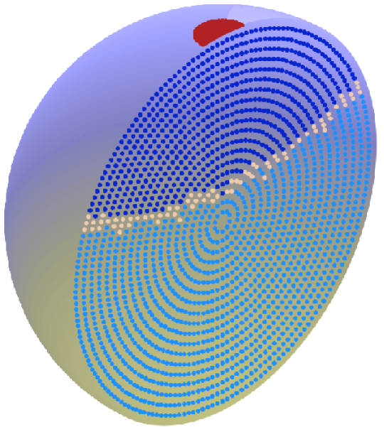
Figure 6: Cut of the phase-chart for the shape of $P(\omega)$ for the NET problem with $p_{a}=0$, $\sigma=1/4\pi$ and $D_{V}=0.000416=D_{S}=0.000625$. Starting locations are coloured light blue if $\chi<-\chi_{\star}$, dark blue if $\chi>\chi_{\star}$ and beige if $|\chi|<\chi_{\star}$, where $\chi_{\star}=0.1$. The red region on the sphere indicates the position of the narrow aperture. The phase-chart has rotation symmetry with respect to the position of the aperture.

In section 2 we discussed a two-dimensional version of this problem. In three dimensions, for a spherical domain of radius $L$, reflecting everywhere except at a narrow circular aperture of radius $\sigma\ll L$ in which the boundary is absorbing, the survival probability at large times is $\mathscr{S}_{\mathbf{r}_{0}}(t)\sim\exp(-t/\tau_{3D})$, where the characteristic time decay $\tau_{3D}=\pi L^{3}/3D\sigma$ corresponds to the MFPT[66].

Here we discuss the statistics of the uniformity index for the NET problem. Consider a sphere of unit radius $\mathcal{S}=\{\mathbf{r}:\rho<1\}$ (in spherical coordinates $\mathbf{r}=(\rho,\theta,\phi)$), and the following boundary conditions: a solid angle $|\Omega|<\sigma$ is absorbing while the remaining part of the sphere is reflective. Furthermore, consider a BM inside $\mathcal{S}$ with a diffusion coefficient $D_{V}$, and initially located at $(\rho_{0},\theta_{0},\phi_{0})$. When the Brownian particle hits the sphere $\partial\mathcal{S}$ it becomes weakly absorbed with probability $p_{a}$ and starts to diffuse, with diffusion coefficient $D_{S}$, along the surface of the sphere. During a time interval $\Delta t$, the particle detaches from the sphere with probability $p_{a}\Delta t$, and continue its motions until it hits the narrow aperture at time $\tau$.

Considering couples of BMs one obtains $P(\omega)$ as before. Fig. 6 shows the phase-chart for the shape of $P(\omega)$, as defined in section 2, for $p_{a}=0$, i.e., when the BM never gets attached to the sphere. The results qualitatively resemble those obtained in section 2 for the two-dimensional disc for narrow apertures (see Fig. 4-$a$). Note that the statistics of the first passage time inherit the polar symmetry of the geometry with respect to the position of the aperture.

Our results indicate that for BMs starting near the location of the aperture, the MFPT has little significance to determine the NET. We have also considered finite values of the attachment probability $p_{a}$ (finite particle-surface affinity), obtaining qualitatively similar results than the ones shown in Fig. 6 for $p_{a}=0$.

6 Conclusions

In this Chapter we discussed a novel diagnostic method which allows to quantify straightforwardly and meaningfully the effects of the trajectory-to-trajectory fluctuations in first passage phenomena characterised by “narrow” distributions $\Psi(\tau)$ possessing moments of arbitrary order. This diagnostic is based on the simultaneity concept of the first passage events. To this purpose, instead of the original random variable $\tau$ characterising the first passage event, we introduced a variable $\omega=\tau_{1}/(\tau_{1}+\tau_{2})$, where $\tau_{1}$ and $\tau_{2}$ are identical independent random variables with the same distribution $\Psi(\tau)$. Physically, the uniformity index $\omega$ shows us the likelihood of the event that two different trajectories arrive to the prescribed location for the first time simultaneously.

We demonstrated that the characteristic shapes of the associated distribution of the uniformity index $\omega$ are very sensitive to the trajectory-to-trajectory fluctuation. In some cases, when such fluctuations have only little effect so that the MFPT can be considered as a meaningful property, the distribution $P(\omega)$ is unimodal with a maximum at $\omega=1/2$, such that $\tau_{1}=\tau_{2}$ is the most probable event. In other cases, $P(\omega)$ is shown to have a bimodal form with two maxima close to $\omega=0$ and $\omega=1$ and a local minimum at $\omega=1/2$. This means that in such situations two different first passage events will be most likely characterised by very different $\tau_{1}$ and $\tau_{2}$, so that the trajectory-to-trajectory fluctuations will be very important and the MFPT cannot be considered as a meaningful characteristic measure of the process. In this regard, the underlying “narrow” distributions $\Psi(\tau)$ may show a behaviour specific to broad distributions which do not possess all moments.

To illustrate this concept, we considered several examples of Brownian motion in bounded domains, in different spatial dimensions and with different locations of the target. We demonstrated that, remarkably, within the same domain the very shape of the distribution $P(\omega)$ depends crucially on the location of the target and on the starting point of the Brownian motion — trajectories starting from one point may exhibit considerable fluctuations with respect to the first passage to the target, while trajectories starting from some other point may arrive to the target location almost simultaneously. For some geometries, we evaluated the “phase charts” for the distribution $P(\omega)$ showing which shape — unimodal or bimodal — this distribution will have for different starting point within each domain.

We expect that a similar behaviour will be observed in bounded one-dimensional geometries for fractional BM with arbitrary Hurst index $H$ or for $\alpha$-stable Lévy flights with $0<\alpha<1$, and more generally, for bounded geometries with compact or non compact exploration.

References

- 1. C. Loverdo, O. Bénichou, M. Moreau, and R. Voituriez, Enhanced reaction kinetics in biological cells, Nature Physics 4, 134 (2008).
- 2. C. Loverdo, O. Bénichou, M. Moreau, and R. Voituriez, Reaction kinetics in active media, J. Stat. Mech. 02, P02045 (2009).
- 3. O. Bénichou, C. Chevalier, J. Klafter, B. Meyer, and R. Voituriez, Geometry-controlled kinetics, Nature Chemistry 2, 472 (2010).
- 4. O. Bénichou, M. Moreau, and G. Oshanin, Kinetics of stochastically gated diffusion-limited reactions and geometry of random walk trajectories, Phys. Rev. E 61, 3388 (2000).
- 5. T. Mattos and F. D. A. A. Reis, Phase transitions and crossovers in reaction-diffusion models with catalyst deactivation, J. Chem. Phys. 131, 014505 (2009).
- 6. M. Smoluchowski, Versuch einer mathematischen Theorie der Koagulations-kinetik kolloidaler Lösungen, Z. Phys. Chem. 92, 129 (1917).
- 7. G. L. Gerstein and B. B. Mandelbrot, Random walk models for the spike activity of a single neuron, Biophys. J. 4, 41 (1964).
- 8. A. N. Burkitt, A review of the integrate-and-fire neuron model: I. Homogeneous synaptic input, Biol. Cybern. 95, 1 (2006).
- 9. G. M. Viswanathan, S. V. Buldyrev, S. Havlin, M. G. E. Da Luz, E. P. Raposo, and H. E. Stanley, Optimizing the success of random searches, Nature 401, 911 (1999).
- 10. G. M. Viswanathan, M. G. E. da Luz, E. P. Raposo, and H. E. Stanley, The Physics of Foraging: An Introduction to Random Searches and Biological Encounters. Cambridge, Cambridge University Press (2011).
- 11. O. Bénichou, M. Coppey, M. Moreau, P. H. Suet, and R. Voituriez, Optimal Search Strategies for Hidden Targets, Phys. Rev. Lett. 94, 198101 (2005).
- 12. C. Loverdo, O. Bénichou, M. Moreau, and R. Voituriez, Robustness of optimal intermittent search strategies in one, two, and three dimensions, Phys. Rev. E 80, 031146 (2009).
- 13. O. Bénichou, C. Loverdo, M. Moreau, and R. Voituriez, Intermittent search strategies, Rev. Mod. Phys. 83, 81 (2011).
- 14. M. A. Lomholt, T. Ambjörnsson, and R. Metzler, Optimal Target Search on a Fast-Folding Polymer Chain with Volume Exchange, Phys. Rev. Lett. 95, 260603 (2005).
- 15. M. A. Lomholt, T. Koren, R. Metzler, and J. Klafter, Lévy strategies in intermittent search processes are advantageous, Proc. Natl. Acad. Sci. USA 105, 11055 (2008).
- 16. M. A. Lomholt, B. van den Broek, S.-M. J. Kalisch, G. J. L. Wuite, and R. Metzler, Facilitated diffusion with DNA coiling, Proc. Natl. Acad. Sci. USA 106, 8204 (2009).
- 17. G. Oshanin, H. S. Wio, K. Lindenberg, and S. F. Burlatsky, Intermittent random walks for an optimal search strategy: one-dimensional case, J. Phys.: Cond. Mat. 19, 065142 (2007).
- 18. G. Oshanin, H. S. Wio, K. Lindenberg, and S. F. Burlatsky, Efficient search by optimized intermittent random walks, J. Phys. A: Math. Theor. 42, 434008 (2009).
- 19. G. Oshanin, O. Vasilyev, P. Krapivsky, and J. Klafter, Survival of an evasive prey, Proc. Natl. Acad. Sci. USA 106, 13696 (2009).
- 20. F. Rojo, C. E. Budde, and H. S. Wio, Optimal intermittent search strategies, J. Phys. A: Math. Theor. 42, 125002 (2009).
- 21. F. Rojo, C. E. Budde, H. S. Wio, G. Oshanin, and K. Lindenberg, Intermittent search strategies revisited: effect of the jump length and biased motion, J. Phys. A: Math. Theor. 43, 345001 (2009).
- 22. C. Mejía-Monasterio, G. Oshanin, and G. Schehr, First passages for a search by a swarm of independent random searchers, J. Stat. Mech. 06, P06022 (2011).
- 23. T. G. Mattos, C. Mejía-Monasterio, R. Metzler, and G. Oshanin, First passages in bounded domains: When is the mean first passage time meaningful?, Phys. Rev. E 86, 031143 (2012).
- 24. J. M. Newby and P. C. Bressloff, Random intermittent search and the tug-of-war model of motor-driven transport, J. Stat. Mech. 04, P04014 (2010).
- 25. I. G. Portillo, D. Campos, and V. Méndez, Intermittent random walks: transport regimes and implications on search strategies, J. Stat. Mech. 02, P02033 (2011).
- 26. M. R. Evans and S. N. Majumdar, Diffusion with Stochastic Resetting, Phys. Rev. Lett. 106, 160601 (2011).
- 27. M. R. Evans and S. N. Majumdar, Diffusion with optimal resetting, J. Phys. A: Math. Theor. 44, 435001 (2011).
- 28. E. Gelenbe, Search in unknown random environments, Phys. Rev. E. 82, 061112 (2010).
- 29. A. L. Lloyd and R. M. May, Epidemiology - How viruses spread among computers and people, Science 292, 1316 (2001).
- 30. A. Hanke and R. Metzler, Bubble dynamics in DNA, J. Phys. A: Math. Theor. 36, L473 (2003).
- 31. H. C. Fogedby and R. Metzler, DNA Bubble Dynamics as a Quantum Coulomb Problem, Phys. Rev. Lett. 98, 070601 (2007).
- 32. G. Oshanin, J. Klafter, and M. Urbakh, Molecular motor with a built-in escapement device, Europhys. Lett. 68, 26 (2004).
- 33. G. Oshanin, J. Klafter, and M. Urbakh, Saltatory drift in a randomly driven two-wave potential, J. Phys.: Condens. Matter. 17, S3697 (2005).
- 34. V. Palyulin and R. Metzler, How a finite potential barrier decreases the mean first-passage time, J. Stat. Mech. 03, L03001 (2012).
- 35. J. P. Bouchaud and M. Potters, Theory of financial risk and derivative pricing: from statistical physics to risk management. Cambridge, Cambridge University Press (2003).
- 36. A. V. Chechkin, R. Metzler, V. Y. Gonchar, J. Klafter, and L. V. Tanatarov, First passage and arrival time densities for Lévy flights and the failure of the method of images, J. Phys. A: Math. Gen. 36, L537 (2003).
- 37. T. Koren, M. A. Lomholt, A. V. Chechkin, J. Klafter, and R. Metzler, Leapover Lengths and First Passage Time Statistics for Lévy Flights, Phys. Rev. Lett. 99, 160602 (2007).
- 38. K. Lindenberg and B. J. West, The first, the biggest, and other such considerations, J. Stat. Phys. 42, 201 (1986).
- 39. S. Redner, A Guide to First-Passage Processes. Cambridge, Cambridge University Press (2001).
- 40. R. Metzler and J. Klafter, Boundary value problems for fractional diffusion equations, Physica A 278, 107 (2000).
- 41. H. Scher, G. Margolin, R. Metzler, J. Klafter, and B. Berkowitz, The dynamical foundation of fractal stream chemistry: The origin of extremely long retention times, Geophys. Res. Lett. 29, 1061 (2002).
- 42. S. Condamin, O. Bénichou, V. Tejedor, R. Voituriez, and J. Klafter, First-passage times in complex scale-invariant media, Nature 450, 77 (2007).
- 43. S. Condamin, O. Bénichou, and M. Moreau, First-Passage Times for Random Walks in Bounded Domains, Phys. Rev. Lett. 95, 260601 (2005).
- 44. S. Condamin, O. Bénichou, and M. Moreau, Random walks and Brownian motion: A method of computation for first-passage times and related quantities in confined geometries, Phys. Rev. E 75, 021111 (2007).
- 45. B. Meyer, C. Chevalier, R. Voituriez, and O. Bénichou, Universality classes of first-passage-time distribution in confined media, Phys. Rev. E 83, 051116 (2011).
- 46. C. Chevalier, O. Bénichou, B. Meyer, and R. Voituriez, First-passage quantities of Brownian motion in a bounded domain with multiple targets: a unified approach, J. Phys. A.: Math. Theor. 44, 025002 (2011).
- 47. J. H. Jeon, A. V. Chechkin, and R. Metzler, First passage behaviour of fractional Brownian motion in two-dimensional wedge domains, Europhys. Lett. 94(2), 20008 (2011).
- 48. I. Eliazar, On selfsimilar Lévy Random Probabilities, Physica A 356, 207 (2005).
- 49. I. Eliazar and I. M. Sokolov, On the fractal characterization of Paretian Poisson processes, Physica A 391, 3043 (2012).
- 50. I. M. Sokolov and I. Eliazar, The matchmaking paradox: a statistical explanation, J. Phys. A.: Math. Theor. 43, 055001 (2010).
- 51. I. M. Sokolov and I. Eliazar, Sampling from scale-free networks and the matchmaking paradox, Phys. Rev. E 81, 026107 (2010).
- 52. G. Oshanin and G. Schehr, Two stock options at the races: Black-Scholes forecasts, Quantitative Finance 12, 1325 (2012).
- 53. G. Oshanin, Y. Holovatch, and G. Schehr, Proportionate vs disproportionate distribution of wealth of two individuals in a tempered Paretian ensemble, Physica A 390, 4340 (2011).
- 54. C. Mejía-Monasterio, G. Oshanin, and G. Schehr, Symmetry breaking between statistically equivalent, independent channels in few-channel chaotic scattering, Phys. Rev. E 84, 035203 (2011).
- 55. D. Boyer, D. S. Dean, C. Mejía-Monasterio, and G. Oshanin, Optimal estimates of the diffusion coefficient of a single Brownian trajectory, Phys. Rev. E 85, 031136 (2012).
- 56. D. Boyer, D. S. Dean, C. Mejía-Monasterio, and G. Oshanin, Distribution of the least-squares estimators of a single Brownian trajectory diffusion coefficient, J. Stat. Mech. 04, P04017 (2013).
- 57. S. N. Majumdar, Persistence in Nonequilibrium Systems, Curr. Sci. 77, 370 (1999).
- 58. A. J. Bray, S. N. Majumdar, and G. Schehr. Persistence and first-passage properties in non-equilibrium systems. arXiv:1304.1195 (2013).
- 59. H. S. Carslaw and J. C. Jaeger, Conduction of Heat in Solids. Oxford University Press, Oxford (1959).
- 60. P. Lévy, Sur certains processus stochastiques homogènes, Comp. Math. 7, 283 (1939).
- 61. J. J. Linderman and D. A. Lauffenburger, Analysis of in- tracellular receptor/ligand sorting, Biophys. J. 50, 295 (1986).
- 62. I. V. Grigoriev, Y. A. Makhnovskii, A. M. Bereshkovskii, and V. Y. Zitserman, Kinetics of escape through a small hole, J. Chem. Phys. 116, 9574 (2002).
- 63. Z. Schuss, A. Singer, and D. Holcman, The narrow escape problem for diffusion in cellular microdomains, Proc. Natl. Acad. Sci. USA 104, 16098 (2007).
- 64. O. Bénichou and R. Voituriez, Narrow-Escape Time Problem: Time Needed for a Particle to Exit a Confining Domain through a Small Window, Phys. Rev. Lett. 100, 168105 (2008).
- 65. G. Oshanin, M. Tamm, and O. Vasilyev, Narrow-escape times for diffusion in microdomains with a particle-surface affinity: Mean-field results, J. Chem. Phys. 132, 235101 (2010).
- 66. H. C. Berg and E. M. Purcell, Physics of chemoreception, Biophys. J. 20, 193 (1977).