Classifying and measuring the geometry of the quantum ground state manifold

Abstract

From the Aharonov-Bohm effect to general relativity, geometry plays a central role in modern physics. In quantum mechanics many physical processes depend on the Berry curvature. However, recent advances in quantum information theory have highlighted the role of its symmetric counterpart, the quantum metric tensor. In this paper, we perform a detailed analysis of the ground state Riemannian geometry induced by the metric tensor, using the quantum XY chain in a transverse field as our primary example. We focus on a particular geometric invariant – the Gaussian curvature – and show how both integrals of the curvature within a given phase and singularities of the curvature near phase transitions are protected by critical scaling theory. For cases where the curvature is integrable, we show that the integrated curvature provides a new geometric invariant, which like the Chern number characterizes individual phases of matter. For cases where the curvature is singular, we classify three types – integrable, conical, and curvature singularities – and detail situations where each type of singularity should arise. Finally, to connect this abstract geometry to experiment, we discuss three different methods for measuring the metric tensor, namely via integrating a properly weighted noise spectral function and by using leading order responses of the work distribution to ramps and quenches in quantum many-body systems.

Understanding the geometry and topology of quantum ground state manifolds is a key component of modern many-body physics. For example, it has become standard practice to characterize topological phases by their Chern number, defined as the integral of Berry curvature over a closed manifold in parameter space. Examples of this include the quantum Hall effect Thouless et al. (1982); Niu et al. (1985), topological insulators Kane and Mele (2005); Sheng et al. (2006), integer and half integer spin chains Berry (1984); Canali et al. (2003), and many others. Non-zero Berry curvature is typically associated with broken time reversal symmetry, either explicitly by external coupling to a time reversal breaking field or implicitly by splitting the ground state manifold into different sectors, each of which breaks time reversal symmetrySheng et al. (2006); Fu and Kane (2006).

However, in addition to the Berry curvature, which describes the flux of Berry phase within the ground state manifold, another important quantity is its symmetric counterpart – the quantum (Fubini-Study) metric tensor – which describes the absolute value of the overlap amplitude between neighboring ground states Provost and Vallee (1980). This metric plays an important role in understanding the physics of quantum many-body ground states Thouless (1998); Ma et al. (2012) and is at the heart of current research in quantum information theory Zanardi et al. (2007a); You et al. (2007); Dey et al. (2012). For instance, the diagonal components of the quantum metric tensor are none other than fidelity susceptibilities, whose scaling in the vicinity of quantum phase transitions – including topological phase transitions – is an object of great interest Yang et al. (2008); Garnerone et al. (2009).

The purpose of this paper is to understand the quantum geometry of a simple model, the spin-1/2 XY chain in a transverse field. For this integrable model, we solve the geometry and topology of the ground state manifold as a function of three parameters: transverse magnetic field, interaction anisotropy, and spin rotation about the transverse axis. Using a standard trick from Riemann geometry, we analyze the three-dimensional metric by taking a series of two-dimensional cuts. For cuts along which the Riemannian manifold is regular, we identify the shape of the manifold and show that the shape of each phase is protected against symmetry-respecting perturbations by critical scaling theory of the metric tensor. For cuts along which the manifold is singular, we identify and classify the singularities. As with the other cuts, we demonstrate that the singularities are robust against a variety of modifications to the low-energy theory. We see three types of geometric singularities: integrable, conical, and curvature singularities. Finally, we detail general circumstances where each type of singularity will arise.

Given the importance of the quantum metric tensor in understanding the properties of ground state manifolds, it is surprising that there have been no direct experimental measurements of the metric tensor to date. Therefore, at the end of the paper we discuss several different proposals for experimentally measuring the components of the metric tensor. The first method is based on the direct representation of the metric tensor through the noise spectral function, generalizing a recent proposal by Neupert et al. Neupert et al. (2013) for measuring the metric tensor in non-interacting Bloch bands. The second method relates the metric tensor to a measurement of the leading non-adiabatic contribution to the excess heat for square root ramps (see also Refs. 17 and 18). The third method similar identifies the metric with leading non-adiabatic corrections to energy fluctuations for generic linear ramps. Finally, the fourth method is based on analyzing the probability of doing zero work in single or double quenches, which is related to the time average of the well-known Loschmidt echo Silva (2008). Using these techniques the full many-body metric tensor is – at least in principle – experimentally accessible. We note that these measurement proposals do not rely on many of the geometric notions discussed elsewhere in the paper, so those primarily interested in measuring the metric can skip directly Sec. IV. We also note that the metric tensor can be readily extracted numerically as a non-adiabatic response of physical observables to imaginary time ramps De Grandi et al. (2011), by directly evaluating overlaps of the ground state wave functions at slightly different couplings Campos Venuti and Zanardi (2007), or through numerical integration of imaginary time noise spectra of the generalized forces Schwandt et al. (2009); Albuquerque et al. (2010).

The rest of this paper proceeds as follows. In Sec. I, we introduce the metric tensor and show its relation to the Berry connection operators. In Sec. I.1, we describe how the Euler characteristic, curvature, and other geometric invariants are obtained from this metric. As a useful example, in Sec. I.3 we explicitly solve for these quantities for the case of the integrable quantum XY model in a transverse field. In Sec. I.4, we show how to visualize the metric manifold by mapping to an isometric surface embedded in three dimensions. These shapes motivate us to define invariant integrals consisting of the contribution to the Euler characteristic within a given phase. We solve this exactly for the XY model then, in Sec. II, we argue based on critical scaling of the metric tensor that the geometric integrals remain unchanged for all models in the same universality class. To further understand the geometry of these Riemann manifolds, we classify three types of singularity in the Gaussian curvature that can occur in the vicinity of phase transitions: integrable (Sec. III.1), conical (Sec. III.2), and curvature (Sec. III.3) singularities. Abstracting away from the XY model, we detail situations under which each type of singularity should arise. Finally, in Sec. IV we discuss different methods for measuring the quantum metric in terms of a more traditional condensed matter measurement of noise correlations, as well as through real-time ramps and quenches of the system parameters as is more relevant to isolated cold atom experiments.

I Geometry of the ground state manifold

Consider a manifold of Hamiltonians described by some coupling parameters $\vec{\lambda}$. A natural measure of the distance between the ground state wave functions $|\psi_{0}\rangle$ separated by infinitesimal $d\vec{\lambda}$ isProvost and Vallee (1980)

$$ds^{2}=1-|\langle\psi_{0}(\vec{\lambda})|\psi_{0}(\vec{\lambda}+d\vec{\lambda})\rangle|^{2}=\sum_{\mu\nu}\chi_{\mu\nu}d\lambda^{\mu}d\lambda^{\nu},$$ (1)

where $\chi_{\mu\nu}$ is the geometric tensor:

$$\chi_{\mu\nu}=\langle\psi_{0}|\overleftarrow{\partial_{\mu}}\partial_{\nu}|\psi_{0}\rangle-\langle\psi_{0}|\overleftarrow{\partial_{\mu}}|\psi_{0}\rangle\langle\psi_{0}|\partial_{\nu}|\psi_{0}\rangle~{},$$ (2)

with $\partial_{\mu}\equiv\frac{\partial}{\partial\lambda^{\mu}}$. As noted by Provost and Vallee Provost and Vallee (1980), this tensor is invariant under arbitrary $\lambda$-dependent $U(1)$ gauge transformation of the ground state wave functions.

Strictly speaking, Eq. 1 utilizes only the real symmetric part of $\chi_{\mu\nu}$, which defines the metric tensor associated with the ground state manifold:

$$g_{\mu\nu}=\Re[\chi_{\mu\nu}]={\chi_{\mu\nu}+\chi_{\nu\mu}\over 2}.$$ (3)

However, in another seminal work Berry (1984), Berry introduced the notion of geometric phase (a.k.a. Berry phase) and the related Berry curvature, which is given by the imaginary (antisymmetric) part of the geometric tensor:

$$F_{\mu\nu}=-2\Im[\chi_{\mu\nu}]=i(\chi_{\mu\nu}-\chi_{\nu\mu})=\partial_{\mu}A_{\nu}-\partial_{\nu}A_{\mu}~{},$$ (4)

where $A_{\mu}=i\langle\psi_{0}|\partial_{\mu}|\psi_{0}\rangle$ is the Berry connection within the ground state manifold. The Berry phase is just a line integral of the Berry connection or – by Stokes theorem – a surface integral of the Berry curvature:

$$\Phi=\oint_{\partial S}\vec{A}\cdot d\vec{\lambda}=\int_{S}F_{\mu\nu}dS_{\mu\nu}~{},$$ (5)

where $dS_{\mu\nu}$ is a directed surface element.

In this work, we will be primarily interested in the metric tensor, $g_{\mu\nu}$. One simple physical interpretation of the metric tensor is that it sets natural units, allowing one to compare different physical parameters. For example, if we consider the ground state manifold as a function of magnetic field and pressure, one can ask how one Tesla compares to one Pascal. In the absence of a simple single particle coupling, the method for scaling these quantities to compare them is not obvious. However, the metric tensor provides a natural answer by allowing one to compare the effects of these couplings on the ground state fidelity. Rescaling the units by the corresponding diagonal components of the metric tensor – a.k.a. the fidelity susceptibilities – one sets natural units for different couplings. Therefore, one Tesla can be compared to one Pascal by comparing the ”dimensionless” couplings after rescaling $d\lambda_{\mu}\to d\lambda_{\mu}/\sqrt{g_{\mu\mu}}$.

I.1 Geometric invariants of the metric tensor

Underlying the classification of most topological phases is the fact that the Berry curvature satisfies the Chern theorem Thouless (1994), which states that the integral of the Berry curvature over a closed two-dimensional manifold $\mathcal{M}$ in the parameter space is $2\pi$ times an integer $n$, known as the Chern number:

$$\oint_{\mathcal{M}}F_{\mu\nu}dS_{\mu\nu}=2\pi n~{}.$$ (6)

Physically this theorem reflects the single valuedness of the wave function during adiabatic evolution: imagine splitting $\mathcal{M}$ into “upper” and “lower” surfaces. To maintain single valuedness, the Berry phases obtained by integrating the Berry curvature over the upper and lower surfaces can only be different by a multiple of $2\pi$.

While the Berry curvature and its associated geometry are certainly of great interest in modern condensed matter physics, the metric tensor $g_{\mu\nu}$ also plays an important role. This tensor defines a Riemannian manifold associated with the ground states, and it is interesting to similarly inquire about its geometry and topology. In particular, the shape of the Riemannian manifold defines a different topological number, given by applying the Gauss-Bonnet theoremCarmo (1976) to the quantum metric tensor:

$$\frac{1}{2\pi}\left[\int_{\mathcal{M}}KdS+\oint_{\partial\mathcal{M}}k_{g}dl\right]=\chi(\mathcal{M})~{},$$ (7)

where $\chi(\mathcal{M})$ is the integer Euler characteristic describing the topology of the manifold $\mathcal{M}$ with metric $g_{\mu\nu}$. The two terms on the left side of Eq. 7 are the bulk and boundary contributions to the Euler characteristic of the manifold. We refer to the first term,

$$\chi_{\mathrm{bulk}}(\mathcal{M})=\frac{1}{2\pi}\int_{\mathcal{M}}KdS~{},$$ (8)

and the second term,

$$\chi_{\mathrm{boundary}}(\mathcal{M})=\frac{1}{2\pi}\oint_{\partial\mathcal{M}}k_{g}dl~{},$$ (9)

as the bulk and boundary Euler integrals, respectively. These terms, along with their constituents – the Gaussian curvature ($K$), the geodesic curvature ($k_{g}$), the area element ($dS$), and the line element ($dl$) – are geometric invariants, meaning that they remain unmodified under any change of variables. More explicitly, if the metric is written in first fundamental form as

$$ds^{2}=Ed\lambda_{1}^{2}+2Fd\lambda_{1}d\lambda_{2}+Gd\lambda_{2}^{2}~{},$$ (10)

then these invariants are given by Kreyszig (1959)

$$K = \frac{1}{\sqrt{g}}\left[\frac{\partial}{\partial\lambda_{2}}\left(\frac{\sqrt{g}\,\Gamma^{2}_{11}}{E}\right)-\frac{\partial}{\partial\lambda_{1}}\left(\frac{\sqrt{g}\,\Gamma^{2}_{12}}{E}\right)\right]$$

$$k_{g} = \sqrt{g}G^{-3/2}\Gamma^{1}_{22}$$

$$dS = \sqrt{g}d\lambda_{1}d\lambda_{2}$$

$$dl = \sqrt{G}d\lambda_{2}~{},$$ (11)

where $k_{g}$ and $dl$ are given for a curve of constant $\lambda_{1}$. The metric determinant $g$ and Christoffel symbols $\Gamma^{k}_{ij}$ are

$$g = EG-F^{2}$$ (12)

$$\Gamma^{k}_{ij} = \frac{1}{2}g^{km}\left(\partial_{j}g_{im}+\partial_{i}g_{jm}-\partial_{m}g_{ij}\right)~{},$$ (13)

where $g^{ij}$ is the inverse of the metric tensor $g_{ij}$.

As we will see, in general the bulk and the boundary terms are not individually protected against perturbations for an arbitrary manifold $\mathcal{M}$. A major purpose of the current work is to demonstrate that if the parameter space manifold terminates at a phase boundary, however, then not only is the sum in Eq. 7 protected against various perturbations, but so is each term individually. Thus, for example, the bulk Euler integral (Eq. 8) can be used for classification of geometric properties of different phases. This geometric invariant is in general different from the Chern number, and can be non-trivial even in the absence of time reversal symmetry breaking.

While the Gauss-Bonnet theorem has a higher dimensional generalization known as the Chern-Gauss-Bonnet theorem Chern (1945), in this work we will focus only on the two-dimensional version. We emphasize that the dimensionality here is that of parameter space; the physical dimensionality of the system can be arbitrary. The choice of parameters is also arbitrary, and is usually dictated either by experimental accessibility, symmetry properties of the system, or other related considerations. Choosing appropriate parameters for studying geometric properties of the phases is therefore similar to choosing parameters defining the phase diagram.

I.2 Defining the geometric tensor through gauge potentials

It can be convenient to express the geometric tensor through the Berry connection operators $\mathcal{A}_{\mu}=i\partial_{\mu}$ associated with the couplings $\lambda_{\mu}$, which one can think of as gauge potentials in parameter space. These gauge operators are formally defined through the matrix elements

$$\mathcal{A}_{\mu}^{mn}=i\langle m|\partial_{\mu}|n\rangle~{},$$ (14)

which implicitly depend on the $U(1)$ phase choice for each energy eigenstate $|n\rangle$ at each $\vec{\lambda}$. If the basis dependence of $\vec{\lambda}$ is expressed through a unitary rotation of some parameter-independent basis,

$$|n(\vec{\lambda})\rangle=U^{nm}(\vec{\lambda})|m\rangle_{0},$$

then the gauge potentials can be written as

$$\mathcal{A}_{\mu}=iU^{\dagger}\partial_{\mu}U.$$ (15)

The operator $\mathcal{A}_{\mu}$ generates infinitesimal translations of the basis vectors within the parameter space. For instance, if spatial coordinates play the role of parameters, then the corresponding gauge potential is the momentum operator. If the parameters characterize rotational angles, the gauge potential is the angular momentum operator.

The ground state expectation value of the gauge operator is by definition the Berry connection

$$A_{\mu}=\langle\psi_{0}|\mathcal{A}_{\mu}|\psi_{0}\rangle.$$ (16)

The geometric tensor is the expectation value of their covariance matrix:

$$\chi_{\mu\nu} = \langle\psi_{0}|\mathcal{A}_{\mu}\mathcal{A}_{\nu}|\psi_{0}\rangle_{c}$$ (17)

$$\equiv \langle\psi_{0}|\mathcal{A}_{\mu}\mathcal{A}_{\nu}|\psi_{0}\rangle-\langle\psi_{0}|\mathcal{A}_{\mu}|\psi_{0}\rangle\langle\psi_{0}|\mathcal{A}_{\nu}|\psi_{0}\rangle.$$

More explicitly, the components of the metric tensor and the Berry curvature are expressed through the connected expectation value of the anti-commutator and the commutator of the gauge potentials, respectively:

$$g_{\mu\nu}={1\over 2}\langle\psi_{0}|\mathcal{A}_{\mu}\mathcal{A}_{\nu}+\mathcal{A}_{\nu}\mathcal{A}_{\mu}|\psi_{0}\rangle_{c},$$ (18)

$$F_{\mu\nu}=i\langle\psi_{0}|\mathcal{A}_{\mu}\mathcal{A}_{\nu}-\mathcal{A}_{\nu}\mathcal{A}_{\mu}|\psi_{0}\rangle.$$ (19)

Although we will be interested only in the ground state manifold for the remainder of this paper, we briefly comment that the definitions above can be extended to arbitrary stationary or non-stationary density matrices. For example, with a finite temperature equilibrium ensemble, one can define $F_{\mu\nu}=i{\rm Tr}(\rho_{\mathrm{thermal}}[\mathcal{A}_{\mu},\mathcal{A}_{\nu}])$.

In Sec. I.3, we will explicitly calculate the gauge potentials of the quantum XY chain. Here we comment on a few of their general properties. First, we note that gauge potentials are Hermitian operators. This follows from differentiating the identity $\langle n(\vec{\lambda})|m(\vec{\lambda})\rangle=\delta_{nm}$ with respect to $\lambda_{\mu}$, or more directly from their definition in terms of unitaries (Eq. 15). Also, the gauge potentials satisfy requirements of locality. In particular, if the Hamiltonian can be written as the sum of local terms $\mathcal{H}=\sum_{i}h_{i}$ and $\vec{\lambda}$ represent global couplings within this Hamiltonian, then the geometric tensor is extensive . In particular, this implies that fluctuations of the gauge potentials are also extensive, which is a general property of local extensive operators. Similarly, if $\vec{\lambda}$ represent local (in space) perturbations, then the geometric tensor is generally system size independent, so that $\mathcal{A}_{\mu}$ is again local. As usual, various singularities – including those breaking locality – can develop in gauge potentials near phase transitions. Finally, we point out that if $\lambda_{\mu}$ is a symmetry of the Hamiltonian, i.e., if the Hamiltonian is invariant under $\lambda_{\mu}\to\lambda_{\mu}+\delta\lambda_{\mu}$, then all gauge potentials $\mathcal{A}_{\nu}$ are also invariant under this symmetry.

I.3 Metric tensor of the quantum XY chain

As our primary example, we consider a quantum XY chain described by the Hamiltonian

$$\mathcal{H}=-\sum_{j}\big{[}J_{x}\mathrm{s}_{j}^{x}s_{j+1}^{x}+J_{y}\mathrm{s}_{j}^{y}s_{j+1}^{y}+hs_{j}^{z}\big{]}~{},$$ (20)

where $J_{x,y}$ are exchange couplings, $h$ is a transverse field, and the spins are represented as Pauli matrices $s^{x,y,z}$. It is convenient to re-parameterize the model in terms of new couplings $J$ and $\gamma$ as

$$J_{x}=J\left(\frac{1+\gamma}{2}\right),\;J_{y}=J\left(\frac{1-\gamma}{2}\right)~{},$$ (21)

where $J$ is the energy scale of the exchange interaction and $\gamma$ is its anisotropy. We add an additional tuning parameter $\phi$, corresponding to simultaneous rotation of all the spins about the $z$-axis by angle $\phi/2$. While rotating the angle $\phi$ has no effect on the spectrum of $H$, it does modify the ground state wave function. To fix the overall energy scale, we set $J=1$.

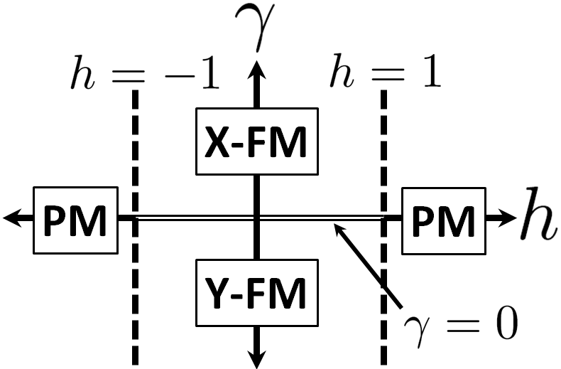
Figure 1: Ground state phase diagram of the XY Hamiltonian (Eq. 22) for $\phi=0$. The rotation parameter $\phi$ modifies the Ising ferromagnetic directions, otherwise maintaining all features of the phase diagram. As a function of transverse field $h$ and anisotropy $\gamma$, the ground state undergoes continuous Ising-like phase transitions between paramagnet and ferromagnet at $h=\pm 1$ and anisotropic transitions between ferromagnets aligned along X and Y directions (X/Y-FM) at $\gamma=0$. These two types of phase transition meet at multi-critical points, which are described in detail in Ref. Mukherjee et al., 2011.

The Hamiltonian described above can be written as

$$\mathcal{H}(h,\gamma,\phi)=-\sum_{j}\left[s_{j}^{+}s_{j+1}^{-}+{\rm h.c.}\right]$$

$$-\gamma\sum_{j}\left[e^{i\phi}s_{j}^{+}s_{j+1}^{+}+{\rm h.c.}\right]-h\sum_{j}s_{j}^{z}~{}.$$ (22)

Since the Hamiltonian is invariant under the mapping $\gamma\to-\gamma$, $\phi\to\phi+\pi$, we generally restrict ourselves to $\gamma\geq 0$, although we occasionally plot the superfluous $\gamma<0$ region when convenient. This model has a rich phase diagram Damle and Sachdev (1996); Mukherjee et al. (2011), as shown in Fig. 1. There is a phase transition between paramagnet and Ising ferromagnet at $|h|=1$ and $\gamma\neq 0$. There is an additional critical line at the isotropic point ($\gamma=0$) for $|h|<1$. The two transitions meet at multi-critical points when $\gamma=0$ and $|h|=1$. Another notable line is $\gamma=1$, which corresponds to the transverse-field Ising (TFI) chain. Finally let us note that there are two other special lines $\gamma=0$ and $|h|>1$ where the ground state is fully polarized along the magnetic field and thus $h$-independent. Thus this line is characterized by vanishing susceptibilities including vanishing metric along the $h$-direction. As we discuss in Sec. III.4 such state is fully protected by the rotational symmetry of the model and can be terminated only at the critical (gapless) point. The phase diagram is invariant under changes of the rotation angle $\phi$.

Rewriting the spin Hamiltonian in terms of free fermions via a Jordan-Wigner transformation, $\mathcal{H}$ can be mapped to an effective non-interacting spin one-half modelSachdev (1999) with

$$\mathcal{H}=\sum_{k}\mathcal{H}_{k}~{};$$ (23)

$$\mathcal{H}_{k}=-\left(\begin{array}[]{cc}h-\cos(k)&\gamma\sin(k)\mathrm{e}^{i\phi}\\ \gamma\sin(k)\mathrm{e}^{-i\phi}&-[h-\cos(k)]\end{array}\right)$$ (26)

This mapping yields a unique ground state throughout the phase diagram by working in a particular fermion parity sectorLieb et al. (1961); none of the conclusions below will change if the other sector is chosen in cases when the ground state is degenerate. A more general analysis involving the non-Abelian metric tensorMa et al. (2010); Neupert et al. (2013) is outside the scope of this work.

The ground state of $\mathcal{H}_{k}$ is a Bloch vector with azimuthal angle $\phi$ and polar angle

$$\theta_{k}=\tan^{-1}\left[\frac{\gamma\sin(k)}{h-\cos(k)}\right]~{}.$$ (27)

To derive the components of the metric tensor, we start by considering the gauge operators introduced in Sec. I.2: $\mathcal{A}_{\mu}\equiv i\partial_{\mu}$. If we consider the transverse field $h$, we see that

$$\partial_{h}|\mathrm{gs}_{k}\rangle=\frac{\partial_{h}\theta_{k}}{2}\left(\begin{array}[]{c}-\sin\left(\frac{\theta_{k}}{2}\right)e^{i\phi/2}\\ \cos\left(\frac{\theta_{k}}{2}\right)e^{-i\phi/2}\end{array}\right)=-\frac{\partial_{h}\theta_{k}}{2}|\mathrm{es}_{k}\rangle~{}.$$ (28)

The same derivation applies to the anisotropy $\gamma$, since changing either $\gamma$ or $h$ only modifies $\theta_{k}$ and not $\phi$. Thus we find

$$\mathcal{A}_{\lambda}=\frac{1}{2}\sum_{k}\big{(}\partial_{\lambda}\theta_{k}\big{)}\tau_{k}^{y}~{},$$ (29)

where $\lambda=\{h,\gamma\}$ and $\tau_{k}^{x,y,z}$ are Pauli matrices that act in the instantaneous ground/excited state basis, i.e., $\tau_{k}^{z}|\mathrm{gs}_{k}\rangle=|\mathrm{gs}_{k}\rangle$, $\tau^{z}_{k}|\mathrm{es}_{k}\rangle=-|\mathrm{es}_{k}\rangle$. Similarly, for the parameter $\phi$, we find that

$$\mathcal{A}_{\phi}=-\frac{1}{2}\sum_{k}\left[\cos(\theta_{k})\tau^{z}_{k}+\sin(\theta_{k})\tau^{x}_{k}\right].$$ (30)

In terms of these gauge potentials, the metric tensor and Berry curvature can be written as (see Sec. I.2)

$$g_{\mu\nu}=\frac{1}{2}\langle\{\mathcal{A}_{\mu},\mathcal{A}_{\nu}\}\rangle_{c}~{}~{},~{}~{}F_{\mu\nu}=i\langle[\mathcal{A}_{\mu},\mathcal{A}_{\nu}]\rangle~{}.$$ (31)

In the case of the XY model, the metric tensor reduces to

$$g_{hh}={1\over 4}\sum_{k}\left({\partial\theta_{k}\over\partial h}\right)^{2}~{};~{}~{}~{}g_{\gamma\gamma}={1\over 4}\sum_{k}\left({\partial\theta_{k}\over\partial\gamma}\right)^{2}$$

$$g_{h\gamma}={1\over 4}\sum_{k}{\partial\theta_{k}\over\partial h}{\partial\theta_{k}\over\partial\gamma}~{};~{}~{}~{}g_{\phi\phi}={1\over 4}\sum_{k}\sin^{2}(\theta_{k})$$

$$g_{h\phi}=g_{\gamma\phi}=0$$ (32)

Although we will not be interested in the Berry curvature in this work, we show the corresponding expressions for completeness

$$F_{h\phi}=-{1\over 2}\sum_{k}{\partial\theta_{k}\over\partial h}\sin(\theta_{k}),$$

$$F_{\gamma\phi}=-{1\over 2}\sum_{k}{\partial\theta_{k}\over\partial\gamma}\sin(\theta_{k}),\;F_{h\gamma}=0.$$ (33)

The expressions for the metric tensor can be evaluated in the thermodynamic limit, where the summation becomes integration over momentum space. It is convenient to divide all components of the metric tensor by the system size and deal with intensive quantities $g_{\mu\nu}\to g_{\mu\nu}/L$. Then one calculates these integrals to find that

$$g_{\phi\phi}=\frac{1}{8}\left\{\begin{array}[]{cc}\frac{|\gamma|}{|\gamma|+1},&|h|<1\\ \frac{\gamma^{2}}{1-\gamma^{2}}\left(\frac{|h|}{\sqrt{h^{2}-1+\gamma^{2}}}-1\right),&|h|>1\end{array}\right.$$ (36)

$$g_{hh}=\frac{1}{16}\left\{\begin{array}[]{cc}\frac{1}{|\gamma|(1-h^{2})},&|h|<1\\ \frac{|h|\gamma^{2}}{(h^{2}-1)(h^{2}-1+\gamma^{2})^{3/2}},&|h|>1\end{array}\right.$$ (39)

$$g_{\gamma\gamma}=\frac{1}{16}\left\{\begin{array}[]{cc}\frac{1}{|\gamma|(1+|\gamma|)^{2}},&|h|<1\\ \left(\begin{array}[]{cc}\frac{2}{(1-\gamma^{2})^{2}}\Big{[}\frac{|h|}{\sqrt{h^{2}-1+\gamma^{2}}}-1\Big{]}-\\ \frac{|h|\gamma^{2}}{(1-\gamma^{2})(h^{2}-1+\gamma^{2})^{3/2}}\end{array}\right),&|h|>1\end{array}\right.$$ (44)

$$g_{h\gamma}=\frac{1}{16}\left\{\begin{array}[]{cc}0,&|h|<1\\ \frac{-|h|\gamma}{h(h^{2}-1+\gamma^{2})^{3/2}},&|h|>1\end{array}\right.$$ (47)

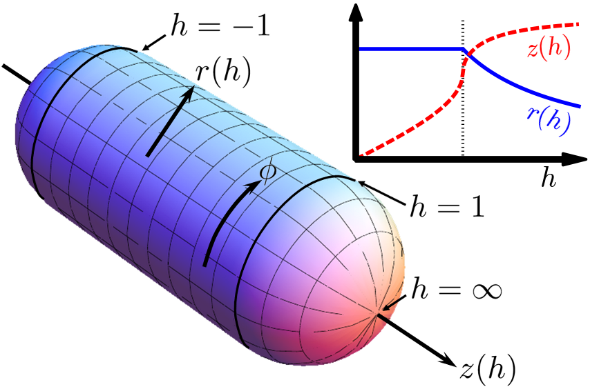
Figure 2: Equivalent graphical representation of the phase diagram of the transverse field Ising model ($\gamma=1$) in the $h-\phi$ plane (Eq. 55). The ordered ferromagnetic phase maps to a cylinder of constant radius. The disordered paramagnetic phases $h>1$ and $h<-1$ map to the two hemispherical caps. The inset shows how the cylindrical coordinates $z$ and $r$ depend on the transverse field $h$.

I.4 Visualizing the ground state manifold

Using the metric tensor we can visualize the ground state manifold by building an equivalent (i.e., isometric) surface and plotting its shape. It is convenient to focus on a two-dimensional manifold by fixing one of the parameters. We then represent the two-dimensional manifold as an equivalent three-dimensional surface. To start, let’s fix the anisotropy parameter $\gamma$ and consider the $h-\phi$ manifold. Since the metric tensor has cylindrical symmetry, so does the equivalent surface. Parameterizing our shape in cylindrical coordinates and requiring that

$$dz^{2}+dr^{2}+r^{2}d\phi^{2}=g_{hh}dh^{2}+g_{\phi\phi}d\phi^{2}~{},$$ (48)

we see that

$$r(h)=\sqrt{g_{\phi\phi}},\;z(h)=\int_{0}^{h}dh_{1}\sqrt{g_{hh}(h_{1})-\left({dr(h_{1})\over dh_{1}}\right)^{2}}.$$ (49)

Using Eq. 36, we explicitly find the shape representing the XY chain. In the Ising limit ($\gamma=1$), we get

$$\left\{\begin{array}[]{l}r(h)={1\over 4}\\ z(h)={\arcsin(h)\over 4}\end{array}\right.\quad|h|<1,$$ (52)

$$\left\{\begin{array}[]{l}r(h)={1\over 4|h|}\\ z(h)={\pi\over 8}{|h|\over h}+{\sqrt{h^{2}-1}\over 4h}\end{array}\right.\quad|h|>1~{}.$$ (55)

The phase diagram is thus represented by a cylinder of radius $1/4$ corresponding to the ferromagnetic phase capped by the two hemispheres representing the paramagnetic phase, as shown in Fig. 2. It is easy to check that the shape of each phase does not depend on the anisotropy parameter $\gamma$, which simply changes the aspect ratio and radius of the cylinder. Because of the relation $r(h)=\sqrt{g_{\phi\phi}}$ this radius vanishes as the anisotropy parameter $\gamma$ goes to zero. By an elementary integration of the Gaussian curvature, the phases have bulk Euler integral $0$ for the ferromagnetic cylinder and $1$ for each paramagnetic hemisphere. These numbers add up to $2$ as required, since the full phase diagram is homeomorphic to a sphere. From Fig. 2, it is also clear that the phase boundaries at $h=\pm 1$ are geodesics, meaning that the geodesic curvature (and thus the boundary contribution $\chi_{\mathrm{boundary}}$) is zero for a contour along the phase boundary. As we will soon see, this boundary integral protects the value of the bulk integral and vice versa.

In the Ising limit ($\gamma=1$), the shape shown in Fig. 2, can also be easily seen from computing the curvature $K$ using Eq. 11. Within the ferromagnetic phase, the curvature is zero – no surprise, given that the metric is flat by inspection. The only shape with zero curvature and cylindrical symmetry is a cylinder. Similarly, within the paramagnet, the curvature is a constant $K=16$, like that of a sphere. Therefore, to get cylindrical symmetry, the phase diagram is clearly seen to be a cylinder capped by two hemispheres.

We can also reconstruct an equivalent shape in the $\gamma-\phi$ plane. In this case we expect to see a qualitative difference for $|h|>1$ and $|h|<1$ because in the latter case there is an anisotropic phase transition at the isotropic point $\gamma=0$, while in the former case there is none. These two shapes are shown in Fig. 3. The anisotropic phase transition is manifest in the conical singularity developing at $\gamma=0$.

The singularity at $\gamma=0$ yields a non-trivial bulk Euler integral for the anisotropic phase transition. To see this, consider the bulk integral

$$\chi_{\mathrm{bulk}}(\epsilon)=\lim_{L\to\infty}\int_{0}^{2\pi}d\phi\int_{\epsilon}^{\infty}d\gamma\,\sqrt{g(\gamma,\phi)}K(\gamma,\phi)~{}.$$ (56)

In the limit $\epsilon\to 0^{+}$, this integral has a discontinuity as a function of $h$ at the phase transition, as seen in Fig. 3. Thus, $\chi_{\mathrm{bulk}}\equiv\chi_{\mathrm{bulk}}(\epsilon=0^{+})$ can be used as a geometric characteristic of the anisotropic phase transition. As we will show in the next section, its value is $\chi_{\mathrm{bulk}}=1/\sqrt{2}$ in the ferromagnetic phase and $\chi_{\mathrm{bulk}}=1$ in the paramagnetic phase. This non-integer geometric invariant is due to the existence of a conical singularity.

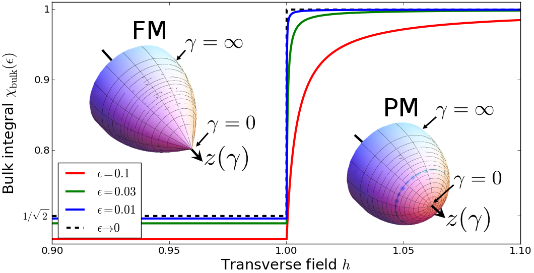
Figure 3: (insets) Equivalent graphical representation of the phase diagram of the XY model in the $\gamma-\phi$ plane, where $\gamma\in[0,\infty)$ and $\phi\in[0,2\pi]$. The right inset shows the paramagnetic disordered phase and the left inset represents the ferromagnetic phase. It is clear that in the latter case there is a conical singularity developing at $\gamma=0$ which represents the anisotropic phase transition. The plots show bulk Euler integral $\chi_{\mathrm{bulk}}(\epsilon)$ as defined in Eq. 56, demonstrating the jump in $\chi_{\mathrm{bulk}}$ at the phase transition between the paramagnet and ferromagnet in the limit $\epsilon\to 0^{+}$.

The last two-dimensional cut, namely the $h-\gamma$ plane at fixed $\phi$, is significantly more complicated and we have not been able to find any simple shape to represent this part of the phase diagram. However, using the technology that we develop below for the more easily visualized surfaces, we analyze the $h-\gamma$ plane in Sec. III.3.

II Universality of the Euler integrals

We now wish to show that the Euler integrals characterizing various phases of the XY model are universal to such phase transitions due to critical scaling of the metric. We begin by considering the transverse-field Ising (TFI) model with $\gamma=1$, $h\in(-\infty,\infty)$, and $\phi\in[0,2\pi)$. For this model, it is knownCampos Venuti and Zanardi (2007) that the metric tensor, and thus the associated curvatures, obey certain scaling laws near the QCP. Therefore, since the boundary of the phase is at such a QCP, critical scaling theory is encoded in the boundary Euler integral.

However, knowing the boundary Euler integral is sufficient to determine the bulk integral. To see this, consider the region $h\in(-1+\epsilon,1-\epsilon)$ for small positive $\epsilon$. Since the region only spans a single phase, there are no ground state degeneracies within this region, meaning the $h-\phi$ surface is homeomorphic to an open cylinder. Because an open cylinder has Euler characteristic $0$, the Gauss-Bonnet theorem becomes

$$\chi_{\mathrm{bulk}}=-\sum_{\mathrm{boundaries}}\chi_{\mathrm{boundary}}.$$ (57)

We want to solve for the bulk Euler integral, in the limit that the boundaries of the region are taken to the phase boundary ($\epsilon\to 0^{+}$). However, according to Eq. 57, the bulk Euler integral is just minus the sum of the boundary integral, which are much easier to solve for. This “bulk-boundary correspondence” is what allows us to use critical scaling theory to determine the bulk Euler integral for each phase.

II.1 Example: Exact metric of the XY chain

As an initial demonstration of this method, consider the exact expression for the metric of the TFI model, given in Eq. 39. For a diagonal metric along a curve of constant $h$, the geodesic curvature reduces to

$$k_{g}^{h\mathrm{\,const.}}=\frac{\partial\sqrt{g_{\phi\phi}}/\partial h}{\sqrt{g_{\phi\phi}g_{hh}}}~{}.$$ (58)

For the case $|h|>1$, this gives

$$k_{g}(h)=\frac{-4/h^{2}}{\sqrt{\frac{1}{h^{4}(h^{2}-1)}}}=-4(h^{2}-1)^{1/2}\stackrel{{\scriptstyle|h|\to 1}}{{\longrightarrow}}0.$$ (59)

Integrating over one of the critical lines, $h=\pm 1$ and $\phi\in[0,2\pi)$, gives $\chi_{\mathrm{boundary}}(|h|=1)=0$. To get some intuition as to what the boundary Euler integral of zero means, consider the three-dimensional embedding shown in Fig. 2. A curve with $k_{g}=0$ is, by definition, a geodesic. This makes sense, since the circle at $h=1$ is clearly a geodesic of both the cylinder and the hemisphere. In general, a smooth curve on a cylindrically-symmetric surface will be a geodesic if the radius is at a local extremum, i.e., $dr/dz=0$. This is clearly satisfied in the case of the TFI model, because $dr/dh$ is finite near the QCP, while $dz/dh\to\infty$ (see Fig. 2, inset).

Similarly, for the limiting point at $h=\infty$, we can calculate the boundary Euler integral:

$$\chi_{\mathrm{boundary}}(h) = \frac{1}{2\pi}\oint k_{g}dl=\frac{1}{2\pi}\int_{0}^{2\pi}k_{g}(h)\sqrt{g_{\phi\phi}(h)}\;d\phi$$ (60)

$$= -\sqrt{\frac{h^{2}-1}{h^{2}}}\stackrel{{\scriptstyle h\to\infty}}{{\longrightarrow}}-1.$$

By the same logic, $\chi_{\mathrm{boundary}}\to-1$ in the limit $h\to-\infty$. Therefore, using Eq. 57, we quickly obtain the $1-0-1$ breakup of the bulk Euler integral for the TFI model.

To further illustrate the analytical power of this method, we can now compute the bulk Euler integral of the $\gamma-\phi$ plane for arbitrary $|h|<1$, as defined in Eq. 56. By a similar analysis as before, one finds that

$$\chi_{\mathrm{boundary}}(\gamma) = \frac{1}{2\pi}\int_{0}^{2\pi}k_{g}(\gamma)\sqrt{g_{\phi\phi}(\gamma)}\;d\phi$$ (61)

$$= -\frac{1}{\sqrt{2(\gamma+1)}}\stackrel{{\scriptstyle\gamma\to 0}}{{\longrightarrow}}-\frac{1}{\sqrt{2}}~{}.$$

Since the limit $\gamma\to\infty$ corresponds to a geodesic (see Fig. 3), giving $\chi_{\mathrm{boundary}}(\gamma\to\infty)=0$, we see that the bulk Euler integral is $\chi_{\mathrm{bulk}}=\frac{1}{\sqrt{2}}$.

II.2 Universality from critical scaling of the metric

We now use critical scaling theory to find the Euler integrals of these phase boundaries for more general models. Consider first the case of an arbitrary model in the TFI (a.k.a. 2D Ising) universality class. We know from the scaling theory of Ref. Campos Venuti and Zanardi, 2007 that the metric diverges near the QCP with a power law set by scaling dimension of the perturbing operators, $\partial_{\lambda}H$. For example, in the transverse-field direction, the metric must scale as $g_{hh}\sim|h-h_{c}|^{-1}$ for arbitrary models in the Ising universality class. Similarly, since the parameter $\phi$ is marginal near the Ising critical point, the singular part of $g_{\phi\phi}$ has scaling dimension $+1$. Adding in the regular part of $g_{\phi\phi}$ to get a non-zero value near the phase transition, we see that to leading order $g_{\phi\phi}\sim A+B|h-h_{c}|$, where $A$ and $B$ are constants. Plugging this into the formula for the boundary Euler integral, one finds that

$$\chi_{\mathrm{boundary}}\sim\frac{\mathrm{const.}}{\sqrt{|h-h_{c}|^{-1}}}\sim|h-h_{c}|^{1/2}\stackrel{{\scriptstyle h\to h_{c}}}{{\longrightarrow}}0.$$ (62)

Therefore, the boundary (and thus bulk) Euler integral of the Ising phase transition is protected by the critical scaling properties of the metric tensor. In terms of the geometry of the three-dimensional embedding, adding irrelevant perturbations to the Hamiltonian will shift the critical point and deform the shape away from the critical point. However, the phase boundary between the ferromagnet and paramagnet will remain a geodesic ($dr/dz$ will remain zero). The fact that the geodesic curvature is zero on the phase boundary has an intuitive physical interpretation. Consider two points on the phase boundary. The geodesic defines the line of the shortest distance between these two points in the Riemannian manifold defined by the metric tensor $g$. It is clear that this line should be entirely confined to the phase boundary since any deviations from it result in moving toward the direction of the relevant coupling, along which the metric tensor diverges. Since the phase boundary coincides with the geodesic, the geodesic curvature is zero by definition.

To understand the more complicated anisotropic direction, we expand the Hamiltonian around $\gamma=0$. Close to the QCP ($|\gamma|\ll 1$), the spectrum is gapless at a single momentum $k_{0}=\cos^{-1}(h)\in(0,\pi)$, around which we can linearize the equations. Then the linearized mode Hamiltonian is

$$H_{k} = -\left(\begin{array}[]{cc}(k-k_{0})\sin k_{0}&\gamma e^{i\phi}\sin k_{0}\\ \gamma e^{-i\phi}\sin k_{0}&-(k-k_{0})\sin k_{0}\end{array}\right)$$

$$= -\left((k-k_{0})\sin k_{0}\right)\sigma^{z}_{k}-\left(\gamma\sin k_{0}\right)\left[\sigma^{x}_{k}\cos\phi-\sigma^{y}_{k}\sin\phi\right]$$

where $\sigma^{(x,y,z)}$ are pseudo-spin Pauli matrices. The presence of $\sin(k_{0})$ in both terms suggests fine-tuning, but this turns out to be unnecessary. Therefore, we consider a more general Hamiltonian of this form:

$$H_{k^{\prime}}=\beta k^{\prime}\sigma_{k^{\prime}}^{z}+\alpha\beta\gamma\left[\sigma^{x}_{k^{\prime}}\cos\phi+\sigma^{y}_{k^{\prime}}\sin\phi\right]~{},$$ (66)

where $\alpha$ and $\beta$ are arbitrary constants and $k^{\prime}\equiv k-k_{0}$ is the momentum difference from the gapless point. This linearized Hamiltonian has

$$\theta_{k^{\prime}}=\tan^{-1}\left(\frac{\alpha\gamma}{k^{\prime}}\right)~{}.$$ (67)

The scaling limits of $g_{\gamma\gamma}$ and $g_{\phi\phi}$ are now relatively straightforward to compute. The formulas are, as before,

$$g_{\gamma\gamma}=\frac{1}{4L}\sum_{k^{\prime}}\left(\frac{\partial\theta_{k^{\prime}}}{\partial\gamma}\right)^{2}~{},\hskip 18.06749ptg_{\phi\phi}=\frac{1}{4L}\sum_{k^{\prime}}\sin^{2}(\theta_{k^{\prime}})~{}.$$ (68)

In the thermodynamic limit, we convert the sum to an integral and define the scaling variable

$$\kappa\equiv k^{\prime}/\gamma~{},$$ (69)

which goes from $\kappa=-\infty$ to $\infty$ in the scaling limit, $|\gamma|\ll 1$. Thus,

$$g_{\phi\phi} = \frac{1}{8\pi}\int_{k^{\prime}}\sin^{2}\theta_{k^{\prime}}dk^{\prime}=\int_{k^{\prime}}\frac{\alpha^{2}\gamma^{2}}{\alpha^{2}\gamma^{2}+k^{\prime 2}}dk^{\prime}$$

$$= \frac{\alpha^{2}\gamma}{8\pi}\int_{-\infty}^{\infty}\frac{1}{\alpha^{2}+\kappa^{2}}d\kappa=\frac{\alpha\gamma}{8}$$

$$g_{\gamma\gamma} = \frac{1}{8\pi}\int_{k^{\prime}}\left(\frac{\partial\theta_{k^{\prime}}}{\partial\gamma}\right)^{2}dk^{\prime}$$ (70)

$$= \frac{\alpha^{2}}{8\pi\gamma}\int_{-\infty}^{\infty}\frac{\kappa^{2}}{\left(\alpha^{2}+\kappa^{2}\right)^{2}}d\kappa=\frac{\alpha}{16\gamma}~{}.$$

Finally, we use our earlier equation for the boundary Euler integral to arrive at

$$\chi_{\mathrm{boundary}}=-\frac{\partial\sqrt{g_{\phi\phi}}/\partial\gamma}{\sqrt{g_{\gamma\gamma}}}=-\frac{\frac{\sqrt{\alpha}}{4\sqrt{2}}\gamma^{-1/2}}{\frac{\sqrt{\alpha}}{4}\gamma^{-1/2}}=-\frac{1}{\sqrt{2}}~{}.$$ (71)

Thus, for all models whose low-energy Hamiltonians are described by Eq. 66, the bulk Euler integral between the anisotropic QCP and the geodesic at $\gamma=\infty$ remains $\frac{1}{\sqrt{2}}$.

II.3 Robustness against angular distortions

The previous section demonstrated robustness of the Euler integrals at phase transitions for the case where the metric is diagonal. In addition, while changes of coordinates can impact the critical scaling properties (at least from a mathematical perspective), the conclusions that we drew were with regards to geometric invariants, and thus manifestly unaffected by such a coordinate change. However, our physical intuition from the theory of continuous phase transitions suggests that this robustness should be even more general, allowing arbitrary perturbations to the model as long as they do not change the scaling properties of the critical point (with regards to traditional observables). Therefore, in this section we demonstrate that perturbations which satisfy this constraint while introducing off-diagonal components to the metric nevertheless do not change the value of the Euler integrals.

In the $h-\phi$ plane, a simple method for introducing off-diagonal terms to the metric is to allow $\gamma$ to vary in the vicinity of the QCP. Let $\gamma$ be some arbitrary function $\gamma(h,\phi)$, with the restriction that $\gamma>0$ so that we remain in the same phase. With this additional freedom, we get a new metric $g^{\prime}(h,\phi)$ such that

$$ds^{2} = g_{hh}dh^{2}+g_{\phi\phi}d\phi^{2}+g_{\gamma\gamma}d\gamma^{2}+2g_{h\gamma}dhd\gamma$$ (72)

$$= g^{\prime}_{hh}dh^{2}+g^{\prime}_{\phi\phi}d\phi^{2}+2g^{\prime}_{h\phi}dhd\phi~{}.$$

Noting that $d\gamma=(\partial_{h}\gamma)dh+(\partial_{\phi}\gamma)d\phi$, we find

$$g^{\prime}_{hh} = g_{hh}+2g_{h\gamma}(\partial_{h}\gamma)+g_{\gamma\gamma}(\partial_{h}\gamma)^{2}$$

$$g^{\prime}_{\phi\phi} = g_{\phi\phi}+g_{\gamma\gamma}(\partial_{\phi}\gamma)^{2}$$

$$g^{\prime}_{h\phi} = g_{\gamma\gamma}(\partial_{h}\gamma)(\partial_{\phi}\gamma)+g_{h\gamma}(\partial_{\phi}\gamma)~{}.$$ (73)

Close to the critical point, only one term diverges: $g_{hh}\sim|h-h_{c}|^{-1}\implies g^{\prime}_{hh}\sim|h-h_{c}|^{-1}$, while both $g^{\prime}_{\phi\phi}$ and $g^{\prime}_{h\phi}$ remain finite near the critical point. Thus, $g^{\prime}$ is asymptotically diagonal near the critical point, our earlier arguments still work, and the boundary Euler integral remains zero.

Not surprisingly, the non-integer bulk Euler integral of the anisotropic phase transition is more sensitive to details of the perturbation. For instance, the most naive option of giving the transverse field a functional dependence ($h\to h(\gamma,\phi)$) changes the value of the bulk Euler integral, which is not surprising given that $h$ is a relevant perturbation at this phase transition. This can be traced back to the fact that modifying $h$ changes the position of the gapless momentum $k_{0}$ (see Eq. II.2), strongly affecting the low-energy physics near the critical point.

In the absence of physical parameters to modify, we instead consider modifications to the low-energy Hamiltonian. In particular, consider a slightly more general Hamiltonian of the form:

$$H_{k^{\prime}}=\beta k^{\prime}\sigma_{k^{\prime}}^{z}+\beta\gamma\left[\alpha_{x}(\phi)\sigma^{x}_{k^{\prime}}\cos\phi+\alpha_{y}(\phi)\sigma^{y}_{k^{\prime}}\sin\phi\right]~{},$$ (74)

where we demand that the functions $\alpha_{x,y}$ are periodic ($\alpha_{x,y}(0)=\alpha_{x,y}(2\pi)$) and positive, such that the azimuthal Bloch angle still wraps the sphere once as we take $\phi$ from $0$ to $2\pi$.

To determine if the Euler integral $\chi_{\mathrm{boundary}}=-1/\sqrt{2}$ is protected, we numerically solve for the boundary Euler integral for a variety of functions $\alpha_{x,y}$. In doing so, we require an additional constraint to ensure that this integral is well-defined: the metric must be positive definite, i.e., its determinant $g=EG-F^{2}$ must be non-zero. We have tested a number of functions satisfying these constraints, and found that all of them have $\chi_{\mathrm{boundary}}=-1/\sqrt{2}$ as expected. Given that the most complex functions we tested ($\alpha_{x}=1+\frac{\cos(\phi^{2}/\pi)}{4}$ and $\alpha_{y}=2+\sin\phi$) have no special symmetries, we postulate that the Euler integral is identical for all functions satisfying the above constraints; however, we are unable to analytically prove such a statement at this time.

III Classification of singularities

Using scaling arguments, we have demonstrated the robustness of the geodesic curvature and the bulk Euler integral for situations where the boundary of the parameter manifold coincides with the phase boundary. One obvious difference between the model in the transverse field ($h-\phi$) and the anisotropy ($\gamma-\phi$) planes is integer vs. non-integer values of the Euler integrals. In this section we show how this difference comes from the nature of the singularities at the respective phase boundaries. We identify two types of geometric singularity: integrable singularities, as in the case of the $h-\phi$ plane, and conical singularities, as in the case of the $\gamma-\phi$ plane. Finally, in the $h-\gamma$ plane, we identify a third type of singularity, known as a curvature singularity. We discuss general conditions under which these singularities should occur and, for the case of conical singularities, identify the relevant parameters in determining the boundary Euler integral.

III.1 Integrable singularities

A simple question which we must ask before classifying the geometric singularities of the XY chain are what, precisely, do we mean by singularities? A simple definition, namely the divergence of one or more components of the metric tensor, is certainly a useful tool for diagnosing the presence of phase transitions in practice Schwandt et al. (2009); Albuquerque et al. (2010). However, we claim that this singularity is less fundamental from a geometric standpoint. For instance, in the case of the TFI model, the transverse field component of the metric tensor diverges as $g_{hh}\sim|h-1|^{-1}$ near $h=1$. However, this divergence can be removed by simply reparameterizing in terms of $h^{\prime}=\sqrt{h-1}\mathrm{sgn}(h-1)$, for which $g_{h^{\prime}h^{\prime}}\sim 1$Dey et al. (2012). Therefore, we need to look elsewhere for information about the fundamental nature of the singularities in the quantum geometry.

Since the issue with the metric tensor was its coordinate dependence, natural quantities to look at are the geometric invariants introduced in Sec. I.1, which are coordinate-independent. Of these, the Gaussian curvature is the obvious choice Zanardi et al. (2007a, b, c); Dey et al. (2012). We therefore classify singularities here and in the rest of the paper based on the Gaussian curvature, $K$, and its invariant integral, $\chi_{\mathrm{bulk}}$.

For the case of the TFI model, the curvature does not diverge near the critical point. This can be easily seen in the equivalent three-dimensional manifold (Fig. 2), where the curvature goes from that of a cylinder ($K=0$) to that of a sphere ($K=1/a^{2}$, where $a$ is the radius), both of which are finite. As we show more explicitly in Sec. III.3, one can derive this non-divergent result by using the scaling forms of the metric tensor to get $K\sim\mathrm{const}$.

However, critical scaling theory does not demand that the curvature is a smooth function of the transverse field. Indeed, we expect it to be singular (like most other quantities) in the vicinity of a phase transition, which manifests in the TFI chain as a jump of $K$ between the ferromagnet and the paramagnet. However, the curvature is finite at all points, and is therefore completely integrable when determining $\chi_{\mathrm{bulk}}$. Therefore, we refer to these jumps in the curvature as “integrable” singularities. We note that visually these integrable singularities correspond to points where the manifold changes shape locally, but in such a way that the tangent plane evolves continuously, so that no cusps or other points of curvature accumulation occur.

III.2 Conical singularities

The anisotropic phase transition at $\gamma=0$ is an example of a conical singularity Fursaev and Solodukhin (1995); Kreyszig (1959), which can easily be seen in Fig. 3. While the specific value of $1/\sqrt{2}$ for the bulk Euler integral is likely specific to this particular class of models, we claim that the existence of conical singularities is in fact a much more general phenomenon.

More specifically, we expect conical singularities to occur in situations with two inequivalent directions orthogonal to a line (or a higher dimensional manifold) of critical points, as long as the orthogonal directions have the same scaling dimension. Denote these directions $\lambda_{1}$ and $\lambda_{2}$, with the critical point at $\lambda_{1}=\lambda_{2}=0$. At $\gamma=0$ in the anisotropic XY model, the parameter $\phi$ has no effect on $H$, so in the FM phase this model satisfies the criteria for a conical singularity with $\lambda_{1}=\gamma\cos\phi$ and $\lambda_{2}=\gamma\sin\phi$.

For simplicity we also assume that the metric has cylindrical symmetry, as in the case of the anisotropic transition in the XY model. In the previous section we verified numerically that this singularity, and in particular the boundary contribution to the Euler characteristic, is protected against breaking of the cylindrical symmetry. We nevertheless use this assumption to simplify our analysis. To ensure cylindrical symmetry, the metric tensor should be diagonal in the $\lambda-\phi$ plane with the leading order asymptotic of the diagonal components of the metric tensor scaling as some power laws:

$$g_{\lambda\lambda}=A\lambda^{-\alpha},~{}~{}g_{\phi\phi}=B\lambda^{\beta}~{},$$ (75)

where $A$ and $B$ are arbitrary positive constants and we generally expect $\alpha\geq 0$, $\beta>0$. However, if we define $\lambda_{1}=\lambda\cos\phi$ and $\lambda_{2}=\lambda\sin\phi$, then the demands of uniform scaling place an additional constraint on the values of the scaling dimensions. To see, this consider the components of the metric in “Cartesian coordinates”:

$$g_{11} = g_{\lambda\lambda}\left(\frac{\partial\lambda}{\partial\lambda_{1}}\right)^{2}+g_{\phi\phi}\left(\frac{\partial\phi}{\partial\lambda_{1}}\right)^{2}$$

$$= g_{\lambda\lambda}\frac{\lambda_{1}^{2}}{\lambda^{2}}+g_{\phi\phi}\frac{\lambda_{2}^{2}}{\lambda^{4}}$$

$$= A\lambda^{-\alpha}\cos^{2}\phi+B\lambda^{\beta-2}\sin^{2}\phi$$

$$g_{22} = A\lambda^{-\alpha}\sin^{2}\phi+B\lambda^{\beta-2}\cos^{2}\phi$$

$$g_{12} = \left(A\lambda^{-\alpha}+B\lambda^{\beta-2}\right)\cos\phi\sin\phi~{}.$$ (76)

We clearly see that the scaling dimensions of $\lambda_{1}$ and $\lambda_{2}$ are the same at all angles $\phi$ if and only if the exponents satisfy the relation:

$$\beta=2-\alpha.$$ (77)

Note that the condition $\beta>0$ now means that $0\leq\alpha<2$. The constants $A$ and $B$ are non-universal, but we expect that their ratio $B/A$ – which defines the anisotropy of the metric tensor – will be a universal number for a given class of models. For the anisotropic transition this ratio is $B/A=2$ and the exponents are $\alpha=\beta=1$ (see Eq. 70). Interestingly the point $h=\infty$ in the $h-\phi$ plane (corresponding the spherical cap – see Fig. 2) also has the form of a conical singularity if we use $\lambda_{1}=\frac{1}{h}\cos(\phi)$ and $\lambda_{2}=\frac{1}{h}\sin(\phi)$ with $\alpha=0$, $\beta=2$, and $B/A=1$. These exponents describe a non-singular point in parameter space with cylindrical symmetry.

Given a conical singularity, we can now easily find the Euler integral. Using the same formulas as earlier for the case of cylindrical symmetry,

$$\chi_{\mathrm{boundary}} = -\frac{\partial\sqrt{g_{\phi\phi}}/\partial\lambda}{\sqrt{g_{\lambda\lambda}}}$$ (78)

$$= \left(\frac{\alpha}{2}-1\right)\sqrt{\frac{B}{A}}~{}.$$ (79)

Using this formula for the anisotropic phase transition of the XY model yields $\chi_{\mathrm{boundary}}=-1/\sqrt{2}$, as found earlier. For a demonstration of the contours of the metric in this model, see Fig. 4.

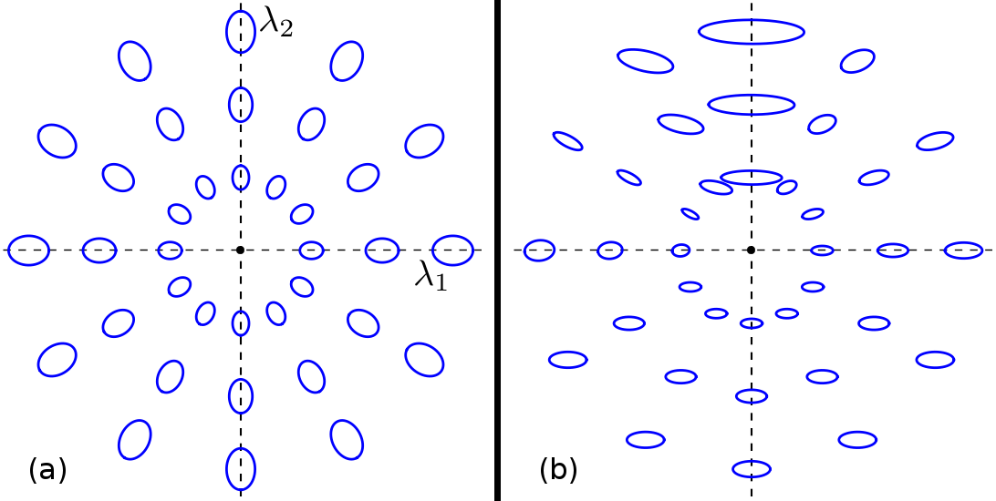
Figure 4: Graphical representation of the metric in the $\lambda_{1}$-$\lambda_{2}$ plane, where a conical singularity (critical point) is at $\lambda_{1}=\lambda_{2}=0$. Panel (a) shows the simple case of the XY model in a transverse field, for which $\alpha=\beta=1$, $B/A=2$, and the metric is cylindrically symmetric about the origin. Panel (b) shows the more general case with Hamiltonian given by Eq. 74, in which the cylindrical symmetry has been broken by using the functions $\alpha_{x}(\phi)=1+\frac{1}{2}\cos(2\phi)-\frac{1}{3}\sin(2\phi)$ and $\alpha_{y}(\phi)=2+\sin(\phi)$. While the cylindrical symmetry is gone, we numerically find that this model has the same conical angle as when $\alpha_{x}=\alpha_{y}=\mathrm{const}$, yielding the same bulk Euler integral. The metric is plotted in both panels by showing the “shape of the circle” near each point, i.e., the blue ellipses show contours of constant radius in the $\lambda_{1}$-$\lambda_{2}$ plane. Since the metric diverges near the critical point, the size of the ellipses gets smaller.

Let us point that if we have a non-singular point like $h\to\infty$ at fixed $\gamma$, for which $\alpha=0$ and $\beta=2$, we have an additional requirement that $g_{11}=g_{22}$ and $g_{12}=0$, implying that $A=B$. This follows from the fact that the metric must remain regular at $\lambda=0$. Then from Eq. 79 we find that the boundary contribution of the isotropic point will be $\chi_{\mathrm{boundary}}=-1$. In a three-dimensional embedding, this indeed looks like a hemisphere, which is non-singular. Therefore, for such smooth “singularities,” the manifold is also guaranteed to be locally equivalent to the hemisphere.

Finally, for the case of a multi-critical point, one can try to apply similar logic. However, due to the asymmetry in the scaling dimensions, along some direction the metric will be infinitely anisotropic near the critical point. This infinite anisotropy is not generally removable by rescaling the couplings. Therefore, the conical singularity breaks down and the curvature can become non-integrably singular.

III.3 Curvature singularities

If we now consider the third two-dimensional cut of the XY model, namely the $h-\gamma$ plane (which has been solved for previously in Ref. Zanardi et al., 2007b), we find that the curvature displays a number of additional singularities. The structure of these singularities can be seen in Fig. 5. It is clear from the plot that as expected there are singularities near the two phase transitions: integrable singularities near the Ising transition ($|h|=1$) and non-integrable singularities near the anisotropic transition ($|h|<1$ and $\gamma=0$). These singularities meet near the multi-critical point ($|h|=1$ and $\gamma=0$) resulting in a very singular and non-monotonic behavior of the curvature.

Figure 5: Three dimensional plot of $K(h,\gamma)$, similar to that found in Fig. 1 of Ref. Zanardi et al., 2007a. The graph shows curvature singularities along the two phase transitions $h=1$ (only positive $h$ are shown) and $h<1$, $\gamma=0$. Unlike the Ising phase transition, the curvature singularities near the anisotropic phase transition are non-integrable, leading to divergent Euler integral within each phase.

While, unlike the $h-\phi$ and $\gamma-\phi$ planes, there are no obvious finite protected Euler integrals in the $h-\gamma$ plane, the exponent of the curvature divergence can be found from scaling arguments. For instance, near the Ising phase transition ($|h|=1$, $\gamma>0$), the simple arguments of Venuti and Zanardi Campos Venuti and Zanardi (2007) indicate that the metric components diverge as $g_{hh}\sim|h-h_{c}|^{-1}$, $g_{\gamma\gamma}\sim 1$, and $g_{h\gamma}\sim 1$. The non-divergence of $g_{\gamma\gamma}$ is due to the fact that $\gamma$ is a marginal parameter, such that the scaling dimension of the singular part of $g_{\gamma\gamma}$ is $+1$. However, there is also a non-zero non-singular part, which is the leading order term near the critical point. Similarly, the scaling dimension of $g_{h\gamma}$ is zero, such that there is a jump singularity near the critical point. Plugging these divergences into Eq. 11 and assuming a smooth dependence on $\gamma$ as long as we are far from the multi-critical point, we find that $K\sim 1$, which matches with the jump singularity in $K$ found at the Ising phase transition. By contrast, near the anisotropic phase transition ($\gamma=0$, $|h|<1$), both the transverse field $h$ and the anisotropy $\gamma$ are relevant parameters, with scaling dimension $-1$. Therefore, the metric components scale as $g_{hh}\sim g_{h\gamma}\sim g_{\gamma\gamma}\sim|\gamma|^{-1}$. By the same logic as before, this leads to a divergent curvature with $K\sim|\gamma|^{-1}$.

Finally, we point out some subtleties regarding the curvature far from critical points. First, while the curvature does not diverge near $h=\infty$ or $\gamma=\infty$, it is not immediately apparent whether the bulk Euler integral diverges in this limit. Therefore, in Appendix B, we show that a simple reparameterization allows one to make both $K$, $\sqrt{g}$, and the limits of integration simultaneously finite, except near quantum critical points at finite $h$ and $\gamma$. Therefore, it becomes clear that the divergence in the Euler integrals comes strictly from the curvature singularities near the quantum phase transitions.

Second, we note that the metric component $g_{hh}$ vanishes at $\gamma=0$ for all $h>1$, since the ground state is the fully-polarized spin-up state along this entire line. The general intuition from Riemann geometry is that if the determinant of the metric vanishes, then the curvature diverges, since the determinant appears in the denominator of the curvature formula (Eq. 11). However, as we show in the next section, the curvature does not in fact diverge for fundamental physical reasons.

III.4 Metric singularity near lines of symmetry

Consider the line $|h|>1$, $\gamma=0$ in the XY model. The ground state along this entire line is fully polarized along the direction of the transverse field, which is clearly the ground state at $h=\infty$. Then, since along this special XY-symmetric line the Hamiltonian commutes with $S^{z}_{\mathrm{total}}$, the fully polarized eigenstate must remain the ground state until a gap closes. Note that this argument continues to hold even in the presence of integrability-breaking perturbations, as long as the $z$-magnetization remains a good quantum number. Therefore, such a line of unchanging ground states and thus vanishing metric determinant is a robust feature of this class of models.

More generally, one can create such fully polarized ground states by considering a family of the Hamiltonians

$$\mathcal{H}(\lambda,\delta)=\mathcal{H}_{0}(\lambda,\delta)-\lambda\mathcal{M}~{},$$ (80)

where $\delta$ is a symmetry breaking field such that $\mathcal{H}_{0}$ and $\mathcal{M}$ commute at $\delta=0$ for any value of $\lambda$. Physically $\mathcal{M}$ represents the generalized force ($z$-magnetization in the above example) which is conserved at the symmetry line. In general $\mathcal{M}$ can also depend on $\lambda$ and $\delta$ as long as $\mathcal{H}_{0}$ and $\mathcal{M}$ commute at $\delta=0$. Clearly in the limit $\lambda\to\infty$ the ground state of the Hamiltonian is the fully polarized state (the state with largest eigenvalue) of the generalized force $\mathcal{M}$, which is generally non-degenerate. By the argument above, along the symmetry line the ground state of $\mathcal{H}$ will be independent of $\lambda$ until the gap in the Hamiltonian closes, e.g., until the system undergoes a quantum phase transition. Thus the metric near this symmetry line will be singular with a vanishing determinant.

We now investigate why, despite this “singular” metric, the curvature nevertheless remains analytic in the vicinity of such a line of symmetry. Assuming we are far from any critical points (i.e., with a gapped spectrum), the components of the metric tensor near the fully polarized state should be analytic and can be written as

$$g=\left(\begin{array}[]{cc}\delta^{2}f_{\lambda\lambda}&\delta f_{\delta\lambda}\\ \delta f_{\delta\lambda}&f_{\delta\delta}\end{array}\right)~{}.$$ (81)

All components $f_{ij}$ are smooth functions of $\lambda$ and $\delta$. For small $\delta$ they can be approximated as being independent of $\delta$, $f_{ij}=f_{ij}(h)$, since the leading asymptotic of the curvature in the limit $\delta\to 0$ will be determined by the explicit dependence given by Eq. 81.

Using the explicit expression for the curvature (Eq. 11) and counting powers of $\delta$, we see that the only possible divergent term in the curvature as $\delta\to 0$ is given by:

$$K\approx-{1\over\delta^{2}\sqrt{f}}{\partial\over\partial\lambda}\left({\sqrt{f}\over f_{\lambda\lambda}}\Gamma^{\delta}_{\lambda\delta}\right),$$ (82)

where $f=\mathrm{det}(f_{ij})$ and

$$\Gamma^{\delta}_{\lambda\delta}={1\over 2g}\left[g_{\lambda\lambda}{\partial g_{\delta\delta}\over\partial\lambda}-g_{\delta\lambda}{\partial g_{\lambda\lambda}\over\partial\delta}\right]={f_{\lambda\lambda}\over 2f}\left[{\partial f_{\delta\delta}\over\partial\lambda}-2f_{\delta\lambda}\right].$$ (83)

Therefore

$$K\approx-{1\over 2\delta^{2}\sqrt{f}}{\partial\over\partial\lambda}\left[{\partial_{\lambda}f_{\delta\delta}-2f_{\delta\lambda}\over\sqrt{f}}\right].$$ (84)

In order to see that the curvature is not divergent near this line of symmetry, we need to show that the following difference vanishes

$$\partial_{\lambda}f_{\delta\delta}-2f_{\delta\lambda}=\partial_{\lambda}g_{\delta\delta}-2\partial_{\delta}g_{\lambda\delta}=0.$$ (85)

This is indeed the case for such general lines of symmetry, as we prove in detail in Appendix A. Therefore, the singular term in the curvature vanishes, and thus the curvature does not diverge near the symmetric line. We emphasize again that our conclusions regarding the curvature are invariant under reparametrization of the couplings.

A more geometric view of the absence of a curvature singularity for metrics satisfying Eq. 85 can be seen by mapping this metric to a Euclidean plane such that all distances are preserved (i.e., an isometric mapping). We start by switching back to the original couplings of the XY-model, $\lambda\leftrightarrow h$ and $\delta\leftrightarrow\gamma$. Then

$$ds^{2} = \gamma^{2}f_{hh}dh^{2}+\gamma\partial_{h}f_{\gamma\gamma}dhd\gamma+f_{\gamma\gamma}d\gamma^{2}$$ (86)

$$= r^{2}d\varphi^{2}+dr^{2},$$

where to the leading order in $\gamma$

$$f_{hh}=\frac{h}{16(h^{2}-1)^{5/2}},\;f_{\gamma\gamma}=\frac{h-\sqrt{h^{2}-1}}{8\sqrt{h^{2}-1}}.$$ (87)

We use the natural ansatz in polar coordinates:

$$r=r(h,\gamma)~{},~{}\varphi=\varphi(h)~{}.$$ (88)

This gives the metric

$$ds^{2} = r^{2}(\partial_{h}\varphi)^{2}dh^{2}+(\partial_{h}r)^{2}dh^{2}+$$ (89)

$$2(\partial_{h}r)(\partial_{\gamma}r)dhd\gamma+(\partial_{\gamma}r)^{2}d\gamma^{2}~{}.$$

Matching the $d\gamma^{2}$ terms, we get $\partial_{\gamma}r=\sqrt{f_{\gamma\gamma}}$, implying that $r=\gamma\sqrt{f_{\gamma\gamma}}$. This also works to match the $dhd\gamma$ terms:

$$2(\partial_{h}r)(\partial_{\gamma}r)=2\gamma\sqrt{f_{\gamma\gamma}}\partial_{h}\sqrt{f_{\gamma\gamma}}=\gamma\partial_{h}f_{\gamma\gamma},$$ (90)

demonstrating the importance of Eq. 85 to obtain a flat metric. Finally, matching the $dh^{2}$ terms, we get

$$\gamma^{2}f_{hh} =r^{2}(\partial_{h}\varphi)^{2}+(\partial_{h}r)^{2}$$

$$=\gamma^{2}(\sqrt{f_{\gamma\gamma}})^{2}(\partial_{h}\varphi)^{2}+\gamma^{2}(\partial_{h}\sqrt{f_{\gamma\gamma}})^{2}$$

$$\varphi =\int_{h}^{\infty}\frac{dh^{\prime}}{\sqrt{f_{\gamma\gamma}(h^{\prime})}}\sqrt{f_{hh}(h^{\prime})-(\partial_{h^{\prime}}\sqrt{f_{\gamma\gamma}(h^{\prime})})^{2}},$$ (91)

where the limits of integration have been chosen to give $\varphi>0$ for all $h$ and $\varphi(h\to\infty)\to 0$. The map is well-defined as long as the term in the square root is positive, i.e., as long as $f_{hh}-(\partial_{h}\sqrt{f_{\gamma\gamma}})^{2}>0$. It’s easy to check that this difference is indeed positive:

$$f_{hh}-(\partial_{h}\sqrt{f_{\gamma\gamma}})^{2}=\frac{h-\sqrt{h^{2}-1}}{32(h^{2}-1)^{5/2}}~{}.$$ (92)

Hence, this embedding works, and shows that the surface for this simplified metric is equivalent to a plane. As such, the curvature is easily seen to be zero.

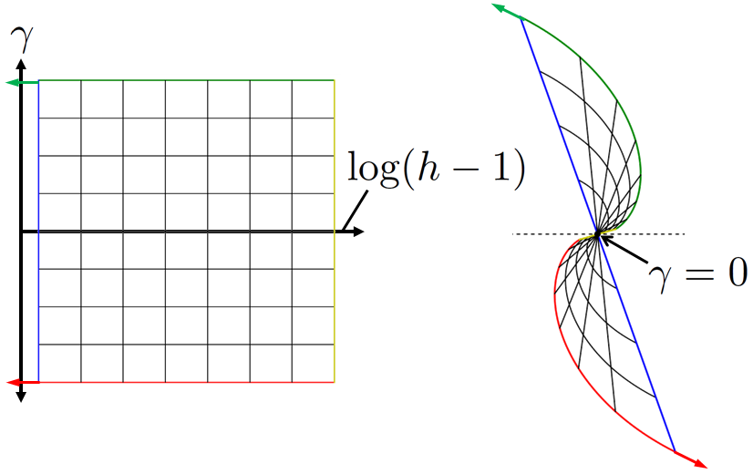
Figure 6: Mapping of the curved space in the $h-\gamma$ plane to a flat plane in polar coordinates. A grid covering a subset of the $h-\gamma$ plane (left) is shown mapped to a subset of the flat plane (right) by a coordinate change to $r$ and $\varphi$ as described in the text. The mapping is specifically shown for the leading order asymptotics of the metric of the XY model given by Eqs. 87, for $h$ ranging from $1.0009$ to $2.0$ and $\gamma$ from $-0.1$ to $0.1$. The red and green arrows indicate that both $\varphi$ and $r$ diverge in the limit $h\to 1^{+}$. Since $g_{hh}=0$ for $\gamma=0$, the entire line $\gamma=0$ maps to a single point, which is a singularity of the model.

While this mapping shows that the manifold in the $h-\gamma$ plane is much less singular than expected, there is still in some sense a singularity at the line of symmetry. This can be see in Fig. 6, where the entire line $\gamma=0$ maps to a single point in the $r-\varphi$ representation. The singularity does not show up directly as a divergence in the scalar curvature. But consider the line $\gamma=0$, and note that any embedding into a higher-dimensional flat space must identify all the points on this line, since $g_{hh}=0$. At the same time, the curvature $K$ is not independent of $h$ along this line (see Fig. 5). Therefore, the curvature cannot be a smooth function for such an embedding, since the curvature upon approaching the point $\gamma=0$ will depend on the direction in which it is approached. By a similar logic, the curvature is singular in the $h-\phi$ plane at $\gamma=0$, diverging as $1/\gamma^{2}$. This is visible in the simple three-dimensional embedding discussed in Sec. I.4; as $\gamma\to 0$, the radius of the hemisphere decreases to zero, and thus the curvature diverges. Finally, as we show in detail in Appendix C, these two divergences conspire to cause the scalar curvature (Ricci scalar) for the full three-dimensional manifold to diverge along this line of symmetry. This divergence is remarkable since the symmetry line does not formally correspond to any phase transition. However, the physical interpretation of these divergences remains unclear to us at this time.

IV Measuring the metric

Formally the metric tensor can be expressed as a standard response function Campos Venuti and Zanardi (2007) and thus is in principle measurable. However, unlike the Berry curvature, which naturally appears in the off-diagonal Kubo-type response De Grandi et al. , the metric tensor appears either as a response in imaginary time dynamics De Grandi et al. (2011, ) or as a response in dissipative systems using specific – and usually not physically justified – requirements for the dissipation Avron et al. (2011). However, as shown in Ref. Neupert et al., 2013 for the specific situation of non-interacting particles, the geometric tensor characterizing the Bloch bands can be measured through the spectral function of the current noise. Here we extend this idea to arbitrary systems and couplings.

The geometric tensor can be represented as (cf. Eq. (B8) in Ref. De Grandi et al., 2011)

$$\chi_{\mu\nu}=\int{d\omega\over 2\pi}{S_{\mu\nu}(\omega)\over\omega^{2}},$$ (93)

where

$$S_{\mu\nu}(\omega)=\int_{-\infty}^{\infty}dt\mathrm{e}^{-i\omega t}\langle\partial_{\mu}H(t)\partial_{\nu}H(0)\rangle_{c}$$ (94)

is the Fourier transform of the connected ground state non-equal time correlation function of the generalized forces, a.k.a. the noise spectral density, and $\partial_{\mu}H(t)=e^{iHt}\partial_{\mu}H(0)e^{-iHt}$ is the generalized force in the Heisenberg picture. The metric tensor is the symmetric (real) part of the geometric tensor and thus can be expressed through the symmetrized spectral density. Following the insight of Neupert et al. Neupert et al. (2013) we interpret $S_{\mu\nu}(\omega)$ as the Fourier transform of the non-equal time noise correlation function of two generalized forces, which is relevant experimentally Blanter and Büttiker (2000). For example, in mesoscopic systems, the current noise spectrum $S_{\mu\nu}(\omega)$ can be measured in shot noise experiments, where current $J_{\mu}$ corresponds to the generalized force $\partial_{A_{\mu}}H$. Eq. 93 suggests a simple and general way of measuring the metric tensor in interacting many-body systems by analyzing equilibrium noise. We believe that, for sufficiently large systems, such symmetrized noise correlations should be measurable with negligible effects of measurement back-action.

While the method of measuring the metric tensor through noise is conceptually simple, it cannot be easily implemented in systems such as cold atoms, where measurements are often destructive. Below, we discuss two real-time protocols which offer the possibility of observing the metric tensor via destructive (single-time) measurements. We then mention an additional protocol involving instantaneous quenches of the external parameters. We note that both ramps Simon et al. (2011); Kim et al. (2011) and quenches Greiner et al. (2002); Sadler et al. (2006); Tuchman et al. (2006) are routinely achieved in isolated cold atom systems.

Consider performing real-time ramps of some parameter $\lambda_{\mu}$ in a gapped system, starting from the ground state at the starting point $\lambda_{i}$. It has been shown elsewhere De Grandi et al. that, for a square root ramp with $\lambda_{\mu}(t)-\lambda_{\mu}(t_{f})=\left[v(t_{f}-t)\right]^{1/2}$, the leading order correction to the energy in the limit $v\to 0$ is given by

$$\langle H\rangle=E_{0}+vg_{\mu\mu}+O(v^{2})~{},$$ (95)

where $H$ is the Hamiltonian, $E_{0}$ is its ground state energy, and $g_{\mu\mu}$ is diagonal component of metric along the ramping direction.

However, the square root ramp is singular near $t_{f}$, and therefore may be difficult to implement. We now show that the metric can also be measured via a more easily implemented linear ramp, at the cost of requiring a harder measurement: the quantum energy fluctuations.

Consider a linear ramp $\lambda_{\mu}(t)-\lambda_{\mu}(t_{f})=v(t-t_{f})$. From Ref. De Grandi and Polkovnikov, 2010, we know that the wave function at $t_{f}$ will be given in its instantaneous eigenbasis by

$$|\psi\rangle=(1+\beta v^{2})|0\rangle-iv\sum_{n\neq 0}\alpha_{n}|n\rangle+O(v^{2})~{},$$ (96)

where $\alpha_{n}=\frac{\langle n|\partial_{\mu}H|0\rangle}{(E_{n}-E_{0})^{2}}$ and $\beta=-(1/2)\sum_{n\neq 0}|\alpha_{n}|^{2}$, which serves to keep the wave function normalized up to order $v^{2}$. The energy fluctuations are given by $\Delta E^{2}=\langle\psi|H^{2}|\psi\rangle-\langle\psi|H|\psi\rangle^{2}$. Without loss of generality, we may offset the Hamiltonian such that the ground state energy is $E_{0}=0$. Then, up to order $v^{2}$,

$$\Delta E^{2} = v^{2}\sum_{n\neq 0}|\alpha_{n}|^{2}\langle n|H^{2}|n\rangle$$ (97)

$$= v^{2}\sum_{n\neq 0}|\alpha_{n}|^{2}E_{n}^{2}$$

$$= v^{2}\sum_{n\neq 0}\frac{\langle n|\partial_{\mu}H|0\rangle\langle 0|\partial_{\mu}H|n\rangle}{E_{n}^{2}}=v^{2}g_{\mu\mu}~{}.$$

Therefore, by measuring the energy fluctuations for different ramp rates and extracting the leading order (quadratic) term, we can extract diagonal terms of the metric along a given direction. Let us point that if we start the ramp in the ground state then the energy fluctuations are equal to the work fluctuations, so the metric tensor can be extracted by measuring work fluctuations as a function of the ramp rate.

A third possibility for measuring the metric tensor is by measuring the probability of doing non-zero work for small quenches in parameter space. This is in some sense true by definition: if $|\psi_{0}(\lambda)\rangle$ is the ground state manifold, then the probability of doing zero work (i.e. ending up in the ground state) after a quench from $\lambda_{\mu}$ to $\lambda_{\mu}+d\lambda_{\mu}$ is just

$$P(W=0) = \big{|}\langle\psi_{0}(\lambda_{\mu})|\psi_{0}(\lambda_{\mu}+d\lambda_{\mu})\rangle\big{|}^{2}$$

$$= 1-g_{\mu\mu}d\lambda_{\mu}^{2}~{};$$

$$P(W\neq 0) = g_{\mu\mu}d\lambda_{\mu}^{2}~{}.$$ (98)

As noted elsewhere, this quantity is equivalent to the time-averaged return amplitude G(t) Silva (2008):

$$P(W=0) = \lim_{T\to\infty}{1\over T}\int_{0}^{T}G(t)dt~{},$$

$$G(t) = \langle\psi_{0}(\lambda_{\mu})|e^{iH(\lambda_{\mu})t}e^{-iH(\lambda_{\mu}+d\lambda_{\mu})t}|\psi_{0}(\lambda_{\mu})\rangle~{},$$

which is related to the well-known Loschmidt echo $L(t)$ by

$$L(t)=|G(t)|^{2}~{}.$$ (99)

The Loschmidt echo is also the probability of returning to the ground state (doing zero work) after a double quench of duration $t$ from $\lambda_{\mu}$ to $\lambda_{\mu}+d\lambda_{\mu}$ and back Heyl et al. . While energy distributions and the related Loschmidt echo are in principle measurable by a variety of methods, we note that there has been important recent progress in proposing measurements of these quantities using few-level systems as a probe Heyl and Kehrein (2012); Mazzola et al. (2013); Dorner et al. (2013).

Finally, we point out that one can reconstruct the full metric tensor solely from measurements of its diagonal components. Consider a two-parameter manifold $(\lambda_{x},\lambda_{y})$. First, measure the diagonal components $g_{xx}$ and $g_{yy}$ using one of the procedures described above. Second, measure a specific off-diagonal element by varying $\lambda_{x}$ and $\lambda_{y}$ simultaneously. For example, if we define the variable $\lambda_{w}=(\lambda_{x}+\lambda_{y})/2$ and ramp or quench along the line $\lambda_{x}=\lambda_{y}$, we can obtain $g_{ww}$. Finally, noting that for this protocol $d\lambda_{x}=d\lambda_{y}=d\lambda_{w}$, we see that

$$ds^{2}=g_{ww}d\lambda_{w}^{2} = g_{xx}d\lambda_{x}^{2}+2g_{xy}d\lambda_{x}d\lambda_{y}+g_{yy}d\lambda_{y}^{2}$$

$$=g_{ww}d\lambda_{x}^{2} = \left(g_{xx}+2g_{xy}+g_{yy}\right)d\lambda_{x}^{2}$$

$$\implies g_{xy} = \frac{g_{ww}-g_{xx}-g_{yy}}{2}~{}.$$ (100)

This procedure can be easily generalized to an $N$-parameter manifold by performing pairwise measurements using a similar tricks as above.

V Conclusions

In conclusion, using the quantum XY model as an example, we have analyzed the Riemann manifold of a simple ground state phase diagram. We identified a new geometric characteristic – the bulk Euler integral – which characterizes the phases of matter. Based on the value of this Euler integral, either integer, non-integer, or undefined, we have classified three types of singularities in the Gaussian curvature: integrable, conical, and curvature singularities. We showed that integrable singularities occur for phase transitions where one parameter is marginal or irrelevant while the other is relevant. Similarly, conical singularities emerge when the phase transition occurs at a single critical point with two “orthogonal” relevant directions that have the same scaling dimensions. And finally near the multi-critical point with two inequivalent relevant directions we found curvature singularities which, similar to black holes, are non-removable non-integrable singularities in the quantum metric space. Finally, by introducing additional techniques for measuring the metric experimentally, we point out that this geometric information should be experimentally accessible.

Appendix A Proof of Eq. 85

We now prove that Eq. 85 indeed holds for the metric given by Eq. 81 near the symmetric line. We will rely on the fact that, at this symmetric line, the ground state does not depend on $\lambda$, so $\partial_{\lambda}|0\rangle=0$. Thus,

$$\partial_{\lambda}g_{\delta\delta}=\partial_{\lambda}\sum_{n\neq 0}\langle 0|\overleftarrow{\partial_{\delta}}|n\rangle\langle n|\partial_{\delta}|0\rangle=\sum_{n\neq 0}\Bigg{[}\left(\langle 0|\overleftarrow{\partial^{2}_{\lambda\delta}}|n\rangle+\langle 0|\overleftarrow{\partial_{\delta}}\partial_{\lambda}|n\rangle\right)\langle n|\partial_{\delta}|0\rangle+\langle 0|\overleftarrow{\partial_{\delta}}|n\rangle\left(\langle n|\overleftarrow{\partial_{\lambda}}\partial_{\delta}|0\rangle+\langle n|\partial^{2}_{\lambda\delta}|0\rangle\right)\Bigg{]}.$$ (101)

$$2\partial_{\delta}g_{\delta\lambda} = \partial_{\delta}\sum_{n\neq 0}\Bigg{[}\langle 0|\overleftarrow{\partial_{\delta}}|n\rangle\langle n|\partial_{\lambda}|0\rangle+\langle 0|\overleftarrow{\partial_{\lambda}}|n\rangle\langle n|\partial_{\delta}|0\rangle\Bigg{]}$$ (102)

$$= \sum_{n\neq 0}\Bigg{[}\left(\langle 0|\overleftarrow{\partial^{2}_{\lambda\delta}}|n\rangle+\langle 0|\overleftarrow{\partial_{\lambda}}\partial_{\delta}|n\rangle\right)\langle n|\partial_{\delta}|0\rangle+\langle 0|\overleftarrow{\partial_{\delta}}|n\rangle\left(\langle n|\overleftarrow{\partial_{\delta}}\partial_{\lambda}|0\rangle+\langle n|\partial^{2}_{\lambda\delta}|0\rangle\right)\Bigg{]}$$

Therefore, we now find that Eq. 85 holds:

$$\partial_{\lambda}g_{\delta\delta}-2\partial_{\delta}g_{\delta\lambda} = \sum_{n\neq 0}\Big{[}\langle 0|\overleftarrow{\partial_{\delta}}\partial_{\lambda}|n\rangle\langle n|\partial_{\delta}|0\rangle+\langle 0|\overleftarrow{\partial_{\delta}}|n\rangle\langle n|\overleftarrow{\partial_{\lambda}}\partial_{\delta}|0\rangle\Big{]}$$ (103)

$$= \sum_{n\neq 0,m}\Big{[}\langle 0|\overleftarrow{\partial_{\delta}}|m\rangle\langle m|\partial_{\lambda}|n\rangle\langle n|\partial_{\delta}|0\rangle+\langle 0|\overleftarrow{\partial_{\delta}}|n\rangle\langle n|\overleftarrow{\partial_{\lambda}}|m\rangle\langle m|\partial_{\delta}|0\rangle\Big{]}=0~{}.$$

The last equality follows by observing that if we interchange indices $n$ and $m$ in the second term in the last sum, we get a term that exactly cancels the first one. This follows from

$$\langle m|\overleftarrow{\partial_{\lambda}}|n\rangle=-\langle m|\partial_{\lambda}|n\rangle.$$ (104)

In addition, the $m=0$ term vanishes because

$$\langle 0|\partial_{\lambda}|n\rangle=-\langle 0|\overleftarrow{\partial_{\lambda}}|n\rangle=0~{}.$$ (105)

Appendix B Choice of parameters

The goal of this section is to show by example that, if the bulk Euler integral $2\pi\chi_{\mathrm{bulk}}=\int KdS$ diverges, then that implies that the curvature must diverge at some point. This is not a priori obvious, because the invariant area $dS=\sqrt{g}d\lambda_{1}d\lambda_{2}$ can also diverge, either because the metric diverges or because the metric is finite but the parameters $\lambda_{i}$ have infinite range. We show that, for the $h-\gamma$ plane of the XY model, such divergences can be removed by a suitable choice of coordinates.

One natural thing to attempt to do is the go to “unitless” coordinate systems, $dh\to\sqrt{g_{hh}}dh$ and $d\gamma\to\sqrt{g_{\gamma\gamma}}d\gamma$, in which a one-parameter metric $g_{\lambda\lambda}$ would become flat (i.e., become $\lambda$-independent). While this does not quite work the same for two parameters, since $g_{hh}$ depends on $\gamma$, we nevertheless use a variant of it below to get a more well-behaved metric. As we will see, the new parameters have a finite range, and the metric is much more well-behaved.

Consider first the case of the transverse field $h$. We wish to define a new parameter $\xi$ such that $d\xi=\sqrt{g_{hh}}dh$. The leading order $h$ dependence of $g_{hh}$ is $g_{hh}\sim\frac{1}{(1-h^{2})}$ in the ferromagnet and $g_{hh}\sim\frac{1}{h^{2}(h^{2}-1)}$ in the paramagnet. Integrating these expressions gives the natural choice

$$\sin\xi\equiv\begin{cases}h&\mbox{if }|h|<1\\ 1/h&\mbox{if }|h|>1~{},\end{cases}$$ (106)

with the quadrant of $\xi$ chosen such that $|\xi|\in[0,\pi/2]$ if $|h|\leq 1$ and $|\xi|\in[\pi/2,\pi]$ if $|h|\geq 1$. We similarly reparameterize the $\gamma$ direction in terms of $\eta$ such that $d\eta=\frac{1}{\sqrt{\gamma}(1+\gamma)}d\gamma$, giving

$$\eta\equiv 2\tan^{-1}(\sqrt{|\gamma|})\mathrm{sgn}\gamma~{}.$$ (107)

The range of our new, auxiliary variables is $\xi\in(-\pi,\pi)$, $\eta\in[0,\pi)$.

Figure 7: Geometric invariants of the XY model in the $\xi$-$\eta$ plane. The three dimensional plots show Gaussian curvature $K$ (a) and metric determinant $g$ (b) for the entire (finite) range of parameters $\xi$ and $\eta$. As discussed in the text, the invariants clearly only diverge near the critical line at $\gamma=0$, except for the determinant $g$, which has an integrable divergence near $\xi=\eta=\pi$.

Within the FM phase, the metric takes on a simple form:

$$g_{\xi\xi}=\frac{1}{16}\cot^{2}\left(\frac{\eta}{2}\right)~{},~{}g_{\eta\eta}=\frac{1}{16}~{}.$$ (108)

By inspection, the metric and its determinant clearly only diverge at the anisotropic phase transition, which is at $\eta=0$ in the new parameters. Within the PM phase, the metric remains quite complicated. However, one can easily calculate the curvature and determinant of the metric, which are given by

$$K = 8+\frac{8\csc(\xi)}{\sqrt{-1+\csc^{2}(\xi)+\tan^{4}\left(\frac{\eta}{2}\right)}}$$

$$g = \csc^{2}(\xi)\sec^{4}\left(\frac{\eta}{2}\right)\tan^{6}\left(\frac{\eta}{2}\right)\left[\frac{-1+2\csc^{2}(\xi)+\tan^{4}\left(\frac{\eta}{2}\right)-2\csc(\xi)\sqrt{-1+\csc^{2}(\xi)+\tan^{4}\left(\frac{\eta}{2}\right)}}{256\left(\tan^{4}\left(\frac{\eta}{2}\right)-1\right)^{2}\left(-1+\csc^{2}(\xi)+\tan^{4}\left(\frac{\eta}{2}\right)\right)^{2}}\right]$$ (109)

These two quantities are plotted for the entire phase diagram in Fig. 7.

Clearly we have almost achieved our goal, in that the invariant area component of the bulk Euler integral, $dS=\sqrt{g}~{}d\xi d\eta$ is finite except near a few select points, namely

• In vicinity of the critical line at $\eta=0$ (i.e. $\gamma=0$), where the curvature also diverges.

• Near the points $|h|,|\gamma|\to\infty$, which correspond to $|\xi|=|\eta|=\pi$. Here the curvature does not diverge, so we expect the divergence of the metric to again be removable.

To see how to remove the divergence in $g$ near $\eta=\xi=\pi$, we need to understand the asymptotics of $g$ near this point. We can do leading order asymptotic expansions of the numerator and denominator about this point. Then if we define

$$u\equiv\frac{1}{\csc(\xi)}\approx\pi-\xi~{},~{}~{}~{}~{}v\equiv\frac{1}{\tan^{2}(\eta/2)}\approx\left(\frac{\pi-\eta}{2}\right)^{2}~{},$$ (110)

we find that the determinant is asymptotically equivalent to

$$g \approx \frac{u^{-2}v^{-5}\big{[}2u^{-2}+v^{-2}-2u^{-1}\sqrt{u^{-2}+v^{-2}}\big{]}}{256v^{-4}\big{[}u^{-2}+v^{-2}\big{]}^{2}}$$ (111)

$$= \frac{\left(\frac{v}{u}\right)\big{[}2\left(\frac{v}{u}\right)^{2}+1-2\left(\frac{v}{u}\right)\sqrt{1+\left(\frac{v}{u}\right)^{2}}\big{]}}{256u\big{[}1+\left(\frac{v}{u}\right)^{2}\big{]}^{2}}~{}.$$ (112)

Rewriting this in circular coordinates $u=r\cos(\theta)$ and $v=r\sin(\theta)$, the expression becomes $g_{\{\xi,\eta\}}=\frac{1}{256r}f(\theta)$, where the notation $g_{\{\xi,\eta\}}$ is meant to reiterate that this is the determinant of the matrix $\left(\begin{array}[]{cc}g_{\xi\xi}&g_{\xi\eta}\\ g_{\eta\xi}&g_{\eta\eta}\end{array}\right)$. The function

$$f(\theta)=\sin\theta\big{[}\sin\theta-1\big{]}^{2}$$ (113)

is defined over the interval $\theta\in[0,\pi/2]$. Then the invariant area is (using the expansions of $u$ and $v$ from above)

$$dS = \sqrt{g_{\{\xi,\eta\}}}d\xi d\eta$$ (114)

$$= \sqrt{\frac{1}{256r}\sin\theta(1-\sin\theta)^{2}}\Big{(}-du\Big{)}\Big{(}-\frac{dv}{2\sqrt{v}}\Big{)}$$

$$= \sqrt{\frac{1}{256r}\sin\theta(1-\sin\theta)^{2}\left(\frac{1}{4r\sin\theta}\right)}dudv$$

$$= \frac{1-\sin\theta}{32r}(rdrd\theta)$$

$$= \frac{1-\sin\theta}{32}drd\theta\equiv\sqrt{g_{\{r,\theta\}}}drd\theta~{}.$$

So we come to our final result that, by choosing a local parameterization $(r,\theta)$ as described above for the points near $|\xi|=|\eta|=\pi$, the metric determinant $g_{\{r,\theta\}}$ is non-divergent. We conclude that, after a suitable choice of local reparameterization, the invariant area term and its integral can be made finite unless curvature diverges. Therefore, all divergences in the bulk Euler integral of the $h-\gamma$ plane are due to the divergent curvature near $\gamma=0$.

Appendix C Full three-dimensional curvature tensor

In this section, we solve for the Riemann curvature tensor, Ricci tensor, and (Ricci) scalar curvature of the full 3D manifold of the XY Hamiltonian Eq. 22. While we remain unable to demonstrate any sharp physical implications of these tensor components, they do give insight geometrically into properties of the 3D Riemann manifold.

C.1 Ferromagnet

For $0<h<1$ and $\gamma>0$ we have for the metric tensor

$$g_{11} = \frac{1}{16}\frac{1}{\gamma(1+\gamma)^{2}}$$

$$g_{22} = \frac{1}{8}\frac{\gamma}{1+\gamma}$$

$$g_{33} = \frac{1}{16}\frac{1}{\gamma(1-h^{2})}~{},$$ (115)

where parameters are labeled $h=\lambda_{1}$, $\gamma=\lambda_{2}$, and $\phi=\lambda_{3}$. This is used then to compute the determinant $g=1/[2048(1-h^{2})\gamma(1+\gamma)^{3}]$ and the inverse metric

$$g^{11} = 16\gamma(1+\gamma)^{2}$$

$$g^{22} = 8\frac{1+\gamma}{\gamma}$$

$$g^{33} = 16\gamma(1-h^{2})$$ (116)

The non-zero components of the Christoffel symbols are

$$\Gamma^{2}_{21} = \Gamma^{2}_{12}=\frac{1}{2\gamma(1+\gamma)},\qquad\Gamma^{3}_{33}=\frac{h}{1-h^{2}},$$

$$\Gamma^{3}_{31} = \Gamma^{3}_{13}=-\frac{1}{2\gamma},\qquad\Gamma^{1}_{22}=-\gamma$$

$$\Gamma^{1}_{33} = \frac{(1+\gamma)^{2}}{2\gamma(1-h^{2})},\qquad\Gamma^{1}_{11}=-\frac{1+3\gamma}{2\gamma(1+\gamma)}~{}.$$ (117)

The nonzero components of the Riemann tensor $R^{\rho}_{\sigma\mu\nu}=\partial_{\mu}\Gamma^{\rho}_{\nu\sigma}-\partial_{\nu}\Gamma^{\rho}_{\mu\sigma}+\Gamma^{\rho}_{\mu\lambda}\Gamma^{\lambda}_{\nu\sigma}-\Gamma^{\rho}_{\nu\lambda}\Gamma^{\lambda}_{\mu\sigma}$ are

$$R^{2}_{323} = -R^{2}_{332}=\frac{1+\gamma}{4\gamma^{2}(1-h^{2})},$$

$$R^{2}_{121} = -R^{2}_{112}=\frac{1}{4\gamma(1+\gamma)^{2}}$$

$$R^{3}_{232} = -R^{3}_{223}=\frac{1}{2}$$

$$R^{3}_{113} = -R^{3}_{131}=\frac{1}{2\gamma^{2}(1+\gamma)}$$

$$R^{1}_{212} = -R^{1}_{221}=\frac{\gamma}{2(1+\gamma)}$$

$$R^{1}_{331} = -R^{1}_{313}=\frac{1+\gamma}{2\gamma^{2}(1-h^{2})}~{}.$$ (118)

The nonzero components of the Ricci tensor $R_{\sigma\nu}=R^{\rho}_{\sigma\rho\nu}$ are

$$R_{11} = \frac{1}{4\gamma(1+\gamma)^{2}}-\frac{1}{2\gamma^{2}(1+\gamma)}$$

$$R_{22} = \frac{1}{2}+\frac{\gamma}{2(1+\gamma)}$$

$$R_{33} = -\frac{1+\gamma}{4\gamma^{2}(1-h^{2})}~{}.$$ (119)

The scalar curvature is obtained by contracting $R^{\mu}_{\nu}=g^{\mu\sigma}R_{\sigma\nu}$ to get $R=R^{\mu}_{\mu}$. We therefore obtain

$$R=-\frac{8}{\gamma}.$$ (120)

This and previous information can be used to compute the Einstein tensor $G_{ij}=R_{ij}-\frac{1}{2}g_{ij}R$, which in our case has the following non=zero components

$$G_{11} = -\frac{1}{4\gamma^{2}(1+\gamma)}~{},~{}G_{22}=1$$

$$\qquad G_{33} = -\frac{1}{4\gamma(1-h^{2})}~{}.$$ (121)

C.2 Paramagnet

For the paramagnet ($\gamma>0$ and $h>1$), the metric is no longer diagonal, although it is block diagonal with the form

$$g=\left(\begin{array}[]{cc}g_{\{1,2\}}&0\\ 0&g_{33}\end{array}\right)~{}.$$ (122)

The inverse metric tensor and Ricci tensor have this same block diagonal form. Their expressions are generally quite complicated, so we will not reproduce them here. However, they can be contracted to give a fairly simple form for the Ricci (1,1) tensor $R^{\mu}_{\nu}$, which has non-zero components

$$R^{1}_{1} = \frac{1}{\gamma^{2}}~{}\frac{4(2-2h^{2}+3\gamma^{2})(h+\sqrt{h^{2}+\gamma^{2}-1})}{\sqrt{h^{2}+\gamma^{2}-1}}$$

$$R^{1}_{2} = -\frac{1}{\gamma}~{}\frac{8(h^{2}-1)}{\sqrt{h^{2}+\gamma^{2}-1}}$$

$$R^{2}_{1} = -\frac{1}{\gamma}~{}\frac{4(\gamma^{2}+2h^{2}-1+2h\sqrt{h^{2}+\gamma^{2}-1})}{\sqrt{h^{2}+\gamma^{2}-1}}$$

$$R^{2}_{2} = 12+\frac{8h}{\sqrt{h^{2}+\gamma^{2}-1}}$$

$$R^{3}_{3} = 8+\frac{12h}{\sqrt{h^{2}+\gamma^{2}-1}}-\frac{8(h^{2}-1+h\sqrt{h^{2}+\gamma^{2}-1})}{\gamma^{2}}~{}.$$ (123)

The trace of $R^{\mu}_{\nu}$ gives the scalar curvature:

$$R=8\left[4+\frac{5h}{\sqrt{h^{2}+\gamma^{2}-1}}-2\frac{\left(h^{2}+h\sqrt{h^{2}+\gamma^{2}-1}-1\right)}{\gamma^{2}}\right]~{}.$$ (124)

Figure 8: Three dimensional scalar curvature $R$ as a function of $h$ and $\gamma$.

Unlike the two-dimensional curvature in the $h-\gamma$ plane, the three dimensional scalar curvature has divergences far from any critical points. For instance, at $h\gg 1$, $R\sim h^{2}$, so it diverges in this limit. Similarly, the scalar curvature diverges near the line of XY symmetry, $R\sim 1/\gamma^{2}$. We note that, similar to the 3D Ricci scalar $R$, the 2D Gauss curvature of the $h-\phi$ plane also diverges as $K\sim 1/\gamma^{2}$. Geometrically, we are not aware of many results regarding three dimensional manifolds with divergent (negative) scalar curvature, but that is indeed what occurs near the line of XY symmetry. Importantly, this is associated with a singular metric, in the sense that both $g_{hh}$ and $g_{\phi\phi}$ vanish at $\gamma=0$. While these divergences are quite interesting and merit further exploration, we have been unable to draw any further physical or geometrical conclusions about them at this time.

References

- Thouless et al. (1982) D. J. Thouless, M. Kohmoto, M. P. Nightingale, and M. den Nijs, Phys. Rev. Lett. 49, 405 (1982).
- Niu et al. (1985) Q. Niu, D. J. Thouless, and Y.-S. Wu, Phys. Rev. B 31, 3372 (1985).
- Kane and Mele (2005) C. L. Kane and E. J. Mele, Phys. Rev. Lett. 95, 146802 (2005).
- Sheng et al. (2006) D. N. Sheng, Z. Y. Weng, L. Sheng, and F. D. M. Haldane, Phys. Rev. Lett. 97, 036808 (2006).
- Berry (1984) M. V. Berry, Proceedings of the Royal Society of London. A. Mathematical and Physical Sciences 392, 45 (1984), URL http://rspa.royalsocietypublishing.org/content/392/1802/45.abstract.
- Canali et al. (2003) C. M. Canali, A. Cehovin, and A. H. MacDonald, Phys. Rev. Lett. 91, 046805 (2003).
- Fu and Kane (2006) L. Fu and C. L. Kane, Phys. Rev. B 74, 195312 (2006).
- Provost and Vallee (1980) J. Provost and G. Vallee, Comm. Math. Phys. 76, 289 (1980).
- Thouless (1998) D. J. Thouless, Topological Quantum Numbers in Nonrelativistic Physics (World Scientific, 1998).
- Ma et al. (2012) Y.-Q. Ma, S.-J. Gu, S. Chen, H. Fan, and W.-M. Liu (2012), arXiv:1202.2397.
- Zanardi et al. (2007a) P. Zanardi, P. Giorda, and M. Cozzini, Phys. Rev. Lett. 99, 100603 (2007a).
- You et al. (2007) W.-L. You, Y.-W. Li, and S.-J. Gu, Phys. Rev. E 76, 022101 (2007).
- Dey et al. (2012) A. Dey, S. Mahapatra, P. Roy, and T. Sarkar, Phys. Rev. E 86, 031137 (2012).
- Yang et al. (2008) S. Yang, S.-J. Gu, C.-P. Sun, and H.-Q. Lin, Phys. Rev. A 78, 012304 (2008).
- Garnerone et al. (2009) S. Garnerone, D. Abasto, S. Haas, and P. Zanardi, Phys. Rev. A 79, 032302 (2009).
- Neupert et al. (2013) T. Neupert, C. Chamon, and C. Mudry (2013), arXiv:1303.4643.
- De Grandi et al. (2011) C. De Grandi, A. Polkovnikov, and A. W. Sandvik, Phys. Rev. B 84, 224303 (2011).
- (18) C. De Grandi, A. Polkovnikov, and A. Sandvik, in preparation.
- Silva (2008) A. Silva, Phys. Rev. Lett. 101, 120603 (2008).
- Campos Venuti and Zanardi (2007) L. Campos Venuti and P. Zanardi, Phys. Rev. Lett. 99, 095701 (2007).
- Schwandt et al. (2009) D. Schwandt, F. Alet, and S. Capponi, Phys. Rev. Lett. 103, 170501 (2009).
- Albuquerque et al. (2010) A. F. Albuquerque, F. Alet, C. Sire, and S. Capponi, Phys. Rev. B 81, 064418 (2010).
- Thouless (1994) D. J. Thouless, Journal of Mathematical Physics 35, 5362 (1994).
- Carmo (1976) M. P. D. Carmo, Differential geometry of curves and surfaces (Prentice-Hall, New Jersey, 1976).
- Kreyszig (1959) E. Kreyszig, Differential Geometry (University of Toronto Press, Toronto, 1959).
- Chern (1945) S. S. Chern, Annals of Mathematics 46, 674 (1945).
- Mukherjee et al. (2011) V. Mukherjee, A. Polkovnikov, and A. Dutta, Phys. Rev. B 83, 075118 (2011).
- Damle and Sachdev (1996) K. Damle and S. Sachdev, Physical Review Letters 76, 4412 (1996), URL http://link.aps.org/doi/10.1103/PhysRevLett.76.4412.
- Sachdev (1999) S. Sachdev, Quantum Phase Transitions (Cambridge University Press, 1999).
- Lieb et al. (1961) E. Lieb, T. Schultz, and D. Mattis, Annals of Physics 16, 407 (1961), ISSN 0003-4916.
- Ma et al. (2010) Y.-Q. Ma, S. Chen, H. Fan, and W.-M. Liu, Phys. Rev. B 81, 245129 (2010).
- Zanardi et al. (2007b) P. Zanardi, L. Campos Venuti, and P. Giorda, Phys. Rev. A 76, 062318 (2007b).
- Zanardi et al. (2007c) P. Zanardi, L. Campos Venuti, and P. Giorda, Phys. Rev. A 76, 062318 (2007c).
- Fursaev and Solodukhin (1995) D. V. Fursaev and S. N. Solodukhin, Phys. Rev. D 52, 2133 (1995).
- Avron et al. (2011) J. E. Avron, M. Fraas, G. M. Graf, and O. Kenneth, New J. Phys. 13, 053042 (2011).
- Blanter and Büttiker (2000) Y. Blanter and M. Büttiker, Physics Reports 336, 1 (2000), ISSN 0370-1573.
- Simon et al. (2011) J. Simon, W. S. Bakr, R. Ma, M. E. Tai, P. M. Preiss, and M. Greiner, Nature 472, 307 (2011), ISSN 0028-0836.
- Kim et al. (2011) K. Kim, S. Korenblit, R. Islam, E. E. Edwards, M.-S. Chang, C. Noh, H. Carmichael, G.-D. Lin, L.-M. Duan, C. C. J. Wang, et al., New Journal of Physics 13, 105003 (2011), ISSN 1367-2630.
- Greiner et al. (2002) M. Greiner, O. Mandel, T. W. Hansch, and I. Bloch, Nature 419, 51 (2002), ISSN 0028-0836.
- Sadler et al. (2006) L. E. Sadler, J. M. Higbie, S. R. Leslie, M. Vengalattore, and D. M. Stamper-Kurn, Nature 443, 312 (2006), URL http://dx.doi.org/10.1038/nature05094.
- Tuchman et al. (2006) A. K. Tuchman, C. Orzel, A. Polkovnikov, and M. A. Kasevich, Phys. Rev. A 74, 051601 (2006).
- De Grandi and Polkovnikov (2010) C. De Grandi and A. Polkovnikov, Lecture Notes in Physics 802, 75 (2010).
- (43) M. Heyl, A. Polkovnikov, and S. Kehrein, arXiv:1206.2505.
- Heyl and Kehrein (2012) M. Heyl and S. Kehrein, Phys. Rev. B 85, 155413 (2012).
- Mazzola et al. (2013) L. Mazzola, G. De Chiara, and M. Paternostro (2013), arXiv:1301.7030.
- Dorner et al. (2013) R. Dorner, S. R. Clark, L. Heaney, R. Fazio, J. Goold, and V. Vedral (2013), arXiv:1301.7021.
- Crooks (2007) G. E. Crooks, Phys. Rev. Lett. 99, 100602 (2007).