Slow Stochastic Switching by Collective Chaos of Fast Elements

Abstract

Coupled dynamical systems with one slow element and many fast elements are analyzed. By averaging over the dynamics of the fast variables, the adiabatic kinetic branch is introduced for the dynamics of the slow variable in the adiabatic limit. The dynamics without the limit are found to be represented by stochastic switching over these branches mediated by the collective chaos of the fast elements, while the switching frequency shows a complicated dependence on the ratio of the two timescales with some resonance structure. The ubiquity of the phenomena in the slow–fast dynamics is also discussed.

Dynamics with distributed timescales are ubiquitous in nature, not only in physicochemical and geophysical systems but also in biological, neural, and social systems. In biological rhythms, for example, dynamics with timescales as long as a day coexist and interfere with the dynamics of much faster biochemical reactions occurring on subsecond timescales Winfree . A similar hierarchy exists even within protein dynamics protein . Electroencephalography (EEG) of the brain is known to involve a broad range of frequencies, and the functional significance of multiple timescales has been extensively discussed brain1 ; brain2 ; brain3 : Neural dynamics in higher cortical areas alter our attention on a slower timescale and switch the neural activities of faster timescales in lower cortical areas. Faster sensory dynamics are stored successively in short-term to long-term memory. Unveiling the salient intriguing behavior that is a result of the interplay of dynamics with different timescales is thus of general importance.

To treat dynamics with fast and slow timescales, several theoretical tools have been developed since the proposition of Born–Oppenheimer approximation in quantum physics. Consider dynamical systems of the form

$$dy_{i}/dt=F_{i}(\{x_{j},y_{j}\});\;\;\epsilon dx_{i}/dt=G_{i}(\{x_{j},y_{j}\}),$$ (1)

where $\epsilon$ is small so that $\{x_{i}\}$ are faster variables than $\{y_{j}\}$. According to adiabatic elimination or Haken’s slaving principle Haken ; GH ; KK81 ; singular , fast variables are eliminated by solving $dx_{i}/dt=0$ for a given $\{y_{j}\}$, and by using this solution of $\{x_{i}\}$ as a function of $\{y_{j}\}$, closed equations for the slow variables are obtained. This is a powerful technique when the fast variables are relaxing to fixed points for the given slow variables, whereas to include a case for which the fast variables have oscillatory dynamics, the averaging method is useful GH ; Average . That is, the long-term average of the fast variables $<x_{i}>$ is taken for a given $\{y_{j}\}$, and by inserting the average into the equation for $\{y_{j}\}$, a set of closed equations for the slow variables is obtained. When the number of variables involved is small, additional techniques developed with the use of a slow manifold can be beneficial Guckenheimer . Dynamical systems with mutual interference between the fast and slow variables have also been investigated Fujimoto1 ; Kanz ; Fujimoto2 ; Vulpiani ; synchro ; Tachikawa ; Spain .

In this Letter, we study a case that involves a large number of fast variables which show chaotic dynamics. We introduce the adiabatic kinetic plot (AKP) to account for the kinetics of the slow variables under the adiabatic limit $\epsilon\rightarrow 0$ by using the averaging method. We show that this plot is useful for analyzing the dynamics even for a finite, small $\epsilon$ for which stochastic transitive dynamics over different modes are observed and are explained as switches over the adiabatic kinetic branches (AKB) obtained from the AKP. This stochasticity in the switches is shown to originate from the collective chaos of an ensemble of fast variables.

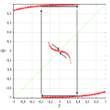
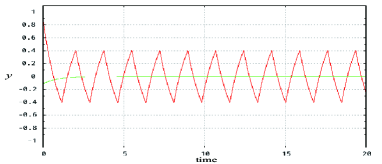
(a) (b)

Fig. 1: (Color online). (a) An example of the AKP for our model (eq.(1)(2)) with $N=10$ and $\beta=10$. The AKP is computed by fixing the $y$ value at the abscissa and numerically integrating the equations of the fast variables for $10^{3}$ time units from 10 randomly selected initial conditions. The ordinate $<h>$ is then computed from the temporal average of the last $8\times 10^{2}$ time units of each initial condition. The $y$ value is incremented by $0.005$ to obtain the plot. (b) The time series of $y$ for $\epsilon=0.0001$. There are two coexisting attractors: a fixed point (green) and a limit cycle (red).

As a specific example, we consider the case for a single slow variable $y$, where $F\equiv h(\{x_{j}\},y)-y$ and $G(\{x_{j}\},y)$ are chosen from the threshold dynamics as

$$\frac{dy}{dt}=h(\{x_{j}\},y)-y\equiv tanh(\frac{\beta}{\sqrt{N}}\sum_{j=1}^{N-1}(J_{0j}x_{j}+J_{00}y))-y,$$ (2)

$$\epsilon\frac{dx_{i}}{dt}=G(\{x_{j}\},y)\equiv tanh(\frac{\beta}{\sqrt{N}}\sum_{j=1}^{N-1}(J_{ij}x_{j}+J_{i0}y))-x_{i},$$ (3)

where $\beta$ is taken to be 10. Here, $J_{ij}$ is chosen as a homogeneous random number in the interval [$-$1,1], and once it is chosen, it is fixed during the dynamics for each sample. We have adopted this form because this type of threshold dynamics thr ; thr2 is used as a simplification of neural network thr-NN or gene regulation network dynamics thr-GRN , in which each element (neuron or gene expression) tends to take either an “on” ($x=1$) or “off” ($x=-1$) state activated ($J_{ij}>0$) or inhibited ($J_{ij}<0$) by other elements. Note, however, that the method and findings discussed here are not restricted to the specific choices of the functions $F$ and $G$; they are valid for any choice.

The dynamics of the slow variable $y$ is represented using the averaging method as $dy/dt=<h(\{x_{j}\}(y))>-y,$ where $<h(\{x_{j}\}(y))>$ is the temporal average of $h$ for a given $y$, i.e., the average input that $y$ receives from $\{x_{j}\}$, in the adiabatic limit. To compute the average $<\cdot>$, we first fix the $y$ value, obtain the attractors for $x_{j}$, and then compute the temporal average for each attractor. By changing the value of $y$, $<h(\{x_{j}\}(y)>$ is obtained, and this forms a continuously changing branch. At this point, it is useful to introduce the plot $(y,<h(\{x_{j}\}(y))>)$ (Fig. 1) If there are multiple attractors that depend on the initial condition of $x_{j}$, then there are several branches in the AKP. Starting from a given $y$ and initial condition $x_{j}$, the dynamical system falls on a specific branch. According to the equation for $y$, if $<h>$ is larger (smaller) than $y$, then $dy/dt>0$ ($dy/dt<0$). Thus, we can trace the dynamics of $y$ along each branch. When a branch crosses the line $y=<h>$, then $y$ falls on a fixed point. If the slope of the branch at the fixed point is less than unity, then the system is attracted to the point so that the slow variable falls on a fixed point attractor (at least) in the limit of $\epsilon\rightarrow 0$ (see the middle branch in Fig. 1). We have confirmed that this is true up to a certain value of $\epsilon$.

The periodic motion of $y$ can also be explained by the AKP. For example, see the top and bottom branches in Fig. 1. As $y$ increases along the top branch, it eventually reaches the endpoint of the branch and then switches to the bottom branch, which corresponds to an alternative attractor of $x$. The process then repeats itself as $y$ decreases along the bottom branch to the endpoint before switching to the top branch. Indeed, this periodic oscillation exists as an attractor, as shown in Fig. 1(b). In this example, the $\{x_{j}\}$ attractor is a fixed point at each branch, but in many other examples, the attractor may be a limit cycle or chaos. However, the present analysis of the $y$ dynamics is still valid in such cases. In fact, the periodic oscillation of $y$ as analyzed from the AKP exists up to a certain value of $\epsilon$ (e.g., $\sim$0.01), where a small amplitude, fast oscillation of order $\epsilon$ is added to the slow $y$ oscillation, if $\{x_{j}\}$ exhibits oscillation.

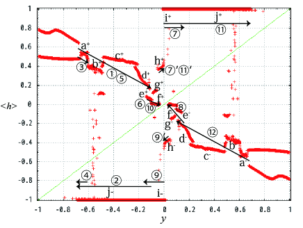
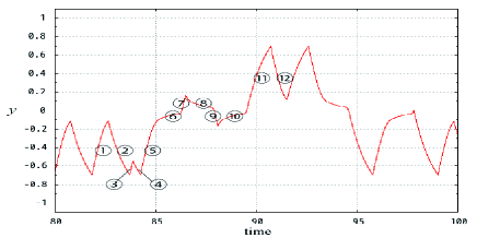
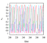
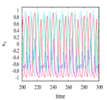
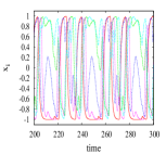
(a) (b) (c1) (c2) (c3)

Fig. 2: (Color online) (a) The AKP with $N=30$ for a given $J$ that produces complex oscillation. The AKP is computed in the same manner as Fig. 1 but from $3\times 10^{5}$ to $3.5\times 10^{5}$ time units over 20 randomly chosen initial conditions. The branches are labeled with lower case letters. Due to the symmetry in the model, branches for $y>0$ and $y<0$ are indicated by $+$ and $-$, respectively. (The branches $i$ and $j$ happen to take almost the same $<h>$ value but belong to different $\{x_{j}\}$ attractors). The numbers correspond to the time course plotted in part (b). (b) Time series of the slow variable $y$ for $\epsilon=0.0001$. The numbers (1, 2, $\cdots$, 12) correspond to the branches visited there, as displayed in part (a). (c) The time series of the fast variables $x_{i}$ ($i=1,2,\cdots,9$) for the branches b, c, and h.

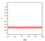
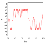
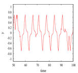
(a) (b) (c)

Fig. 3: (Color online): Time series of the slow variables $y$ corresponding to Fig,2, except for $\epsilon=2\times 10^{-6}$ (a), $\epsilon=1\times 10^{-5}$ (b), and $\epsilon=1\times 10^{-4}$ (c). The time series of (c) corresponds to Fig.2(b) but is plotted for a longer time span.

In general, AKP has much more branches that make the oscillatory dynamics complex. A rather more complicated example is shown in Fig. 2. In this case, in the limit of $\epsilon\rightarrow 0$, $y$ switches between two branches. In the example in Fig. 3 (a) for $\epsilon=2\times 10^{-6}$, $y$ periodically switches between the branch $a^{+}$ and a section of branch $j^{-}$ (“4”). For a larger $\epsilon$ value, however, complex oscillations of $y$ are seen, as shown in Fig. 2. This is described as the switching over all 2 $\times$ 10 branches, a^±, b^±, c^±, …, j^± (the first 12 are labeled explicitly in the figure), where $\pm$ denotes the symmetric branches of $y>0$ and $y<0$. Here, we should mention that this switching is not always deterministic. For example, $a^{+}\rightarrow b^{+}$ (“1”) or $a^{+}\rightarrow i^{-}$ (“3” $\rightarrow$ “4”) are both possible, as are $d^{+}\rightarrow j^{-}$ (“1” $\rightarrow$ “2”) and $d^{+}\rightarrow e^{+}$ (“5” $\rightarrow$ “6”). As $\epsilon$ is decreased, a larger number of branches is visited by the stochastic switches (see Fig. 3(a) to 3(b) and to 3 c)] until only a cycle between two branches remains in the limit of $\epsilon\rightarrow 0$, as in Fig. 3(a).

With the complex switches, the dynamics of $x_{i}$ switch among (at least) 2 $\times$ 10 types of attractors including fixed points, limit cycles, and chaos. This type of switching is reminiscent of chaotic itinerancy Ikeda ; Tsuda ; GCM ; CI where the orbit itinerates over “attractor ruins”. Here, in contrast, the stochastic switches progress among attractors for a given value of the slow variable $y$, while the chaotic dynamics of the fast variables provides a source for the stochastic switching. Indeed, at the boundary of the branches $a,d,f,\cdots$, the fast variables $\{x_{i}\}$ show chaotic oscillation.

For a detailed analysis of the stochastic switching due to the chaotic dynamics, we consider the simpler example given in Fig. 4 with a different matrix $J_{ij}$. In this case, as $\epsilon\rightarrow 0$, $y$ shows periodic oscillation between the two branches $a^{+}$ and $a^{-}$, whereas for $\epsilon>\epsilon_{c}\approx 0.5\times 10^{-5}$, the branches $b^{+}$ and $b^{-}$ are also available, and stochastic switching $a^{+}\rightarrow a^{-},b^{+}$ and its symmetric counterpart appear. The choice between $a^{+}\rightarrow a^{-}$ and $a^{+}\rightarrow b^{+}$ is stochastic, and indeed, we have computed the Shannon entropy of the $n$-tuple symbol sequence of the branches $a,b$ visited by the slow $y$ variable and confirmed that it increases linearly with $n$ ($\sim 0.91n$)transient .

To examine if the origin of the stochasticity lies in the chaos of the fast variables, we measured the maximal Lyapunov exponent for the $(N-1)$-dimensional fast dynamics of $\{x_{i}\}$ for a given $y$ at each branch. As shown in Fig. 4 (c), the exponent is positive around the endpoints of the branches where stochastic switching occurs. Several other examples also show stochastic transitioning beyond a critical value of $\epsilon$, a Poisson switching-time distribution, and a positive Lyapunov exponent at the branch endpoint (for example see Supplementary Figs. 2). The stochastic switching from the branches a and f in Fig. 2 is also explained by the chaotic dynamics of the fast $\{x_{i}\}$ variables at the branches.

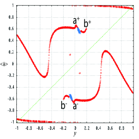
(a)

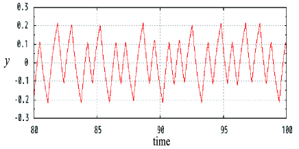
(b)

Fig. 4: (Color online) (a) The AKP computed for a different matrix $J$ with $N=20$ and the time average between $10^{2}$ to $2\times 10^{3}$ time units from 15 initial conditions. The maximum Lyapunov exponent of the dynamics of $\{x_{i}\}$ is also computed over the interval of $3\times 10^{3}$ to $4\times 10^{3}$ time units for each branch of a given $y$. The segment of the branch with positive exponent (whose value is about $\sim.02$) is colored as blue. (See Supplementary Fig.1 for the Lyapunov exponents at each branch). (b) The time series of $y$ for $\epsilon=0.001$.

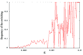
Fig. 5: (Color online) Frequency of the switching in the branches corresponding to the dynamics in Fig. 4 as a function of $\epsilon$. For each $\epsilon$ value, the number of a+ to b+ switching events divided by those from a+ to a- are computed as the fraction of the number of times that $y$ goes beyond $0.2$ divided by the number of times that it goes below $0$ within 500 time units.

When $\{x_{i}\}$ shows chaotic dynamics, one might expect that the variable $h$ can be regarded as just the noise represented by the sum of random $\{x_{i}\}$ variables. If this were the case, then the amplitude of this noise would decrease as the number of fast elements $N$ is increased. The variable $h$ would then approach a constant in the $N\rightarrow\infty$ limit, and the frequency of the stochastic switchings would decrease accordingly. However, this is does not occur. We simulated the present model by increasing the number of fast elements by $2^{k}$ ($k=1,2,\cdots,6$) by cloning the matrix $J_{ij}$ and confirmed that the frequency does not decrease with an increase in $N$. This suggests that there is still some correlation among the fast variables $x$, so that $h$ shows collective chaotic motion, as has been studied extensively KK-PRL ; CM ; Shibata ; KK-book . In fact, the oscillation of the collective variable $h$ has a larger amplitude than the typical mean-field oscillation in the collective chaos in coupled chaotic systems studied thus far KK-PRL ; Shibata . Indeed, some of the fast elements $x_{i}$ undergo a large-amplitude change between the on and off (1 and $-$1) states and there remains correlation among the $x_{i}$ variables.

With an increase in $\epsilon$ beyond $\epsilon_{c}$, the frequency of the stochastic switching increases, but with a further increase, the frequency shows a complicated dependence on $\epsilon$, as it is increased beyond $\epsilon_{c}$. There are certain parameters for which the switching loses its stochasticity and is replaced by either perfect switching between two original branches in the $\epsilon\rightarrow 0$ limit or perfect switching to the new branch (i.e., $a^{+}\rightarrow b^{+}$ only). When the switching ratio is zero or unity, the long-term oscillation of the slow variable $y$ is periodic. Thus, each such “deterministic” region is regarded as a “window” in the parameter region showing chaos. Here, it is interesting to note that periodic motion is generated between variables with timescales differing by more than one order of magnitude. In fact, the collective variable $h$ can have a slower component than the original timescale $\epsilon$ for $x_{i}$. Complicated resonance structures of the switching ratio are often observed in the present system when stochastic switchings exist.

To summarize, we have introduced an AKP to study the kinetics of slow variables in the adiabatic limit $\epsilon\rightarrow 0$, Up to a certain critical value $\epsilon_{c}$, the slow dynamics fall either on a fixed point or exhibit periodic switching between branches. As $\epsilon$ is increased (i.e., the timescale difference is decreased), stochastic switching among several branches appears mediated by the collective chaotic motion of the fast variables, and the variety of switchings increases with a further increase in $\epsilon$.

Although we have employed a simplified threshold dynamics model that borrows concepts from neural or gene regulation networks, the AKP method can be applied generally to fast–slow systems, and stochastic switching over the AKB will appear when the fast variables show chaotic motion. Extension to a case with multiple slow variables is also possible, in principle, by extending each branch to a surface or higher-dimensional manifold. Although visualization in this case will be difficult in comparison with the present AKP, the stochastic transitions over adiabatic manifolds can be analyzed using the methods developed here.

As a result of the switching, long-term itinerancy over different modes of oscillation of the fast variables appears, which is reminiscent of chaotic itinerancy. Experimentally, such itinerancy is often observed in EEGs of the brain, biorhythms, climate dynamics, and so forth, where modes with different timescales coexist CI . The present approach may shed light on such itinerant behavior, while hierarchical construction of AKPs may be beneficial to deal with a system with a variety of distinct timescales Fujimoto2 .

Collective chaotic motion of fast variables is a source of stochastic switching and is modulated by the motion of slow variables; such mutual inference between fast and slow modes leads to resonance between the slow and collective modes, which is similar to the interference in the neural activity dynamics between higher and lower cortical areas during changes in our attention.

We would like to thank Shuji Ishihara, Nen Saito, and Shin’ichi Sasa for useful discussions. This work was partially supported by a Grant-in-Aid for Scientific Research (No. 21120004) on Innovative Areas “Neural creativity for Communication” (No. 4103) and the Platform for Dynamic Approaches to Living System from MEXT, Japan.

References

- [1] A. T. Winfree, Geometry of Biological Time, Springer, New York, 1980
- [2] K. A. Henzler-Wildman et al., Nature 450 (2007) 913
- [3] S. J. Kiebel, J. Daunizeau, and K. J. Friston, PLoS Comput Biol 4 (2008) e1000209
- [4] M. Breakspear and C. J. Stam, Phil. Trans. R. Soc. B 360 (2005) 1643
- [5] L Kay, Chaos 13 (2003) 1057
- [6] H. Haken, Synergetics, Springer, New York, 1977
- [7] J. Guckenheimer and P. Holmes, Nonlinear Oscillations, Dynamical Systems, and Bifurcation of Vector Field, Springer, New York, 1986
- [8] K. Kaneko, Prog. Theor. Phys. 66 (1981) 129
- [9] N. Fenichel, J. Differential Equations, 31 (1979) 53
- [10] A. Sanders and F. Verhulst, Averaging Methods in Nonlinear Dynamical Systems, Springer, New York, 1985
- [11] M. Desroches et al., SIAM Review 54 (2012) 211
- [12] K. Fujimoto and K. Kaneko, Physica D 180 (2003) 1
- [13] W. Just, K. Gelfert, N. Baba, A. Riegert, and H. Kantz, J. Stat. Phys. 112 (2003) 277
- [14] K. Fujimoto and K. Kaneko, Chaos 13 (2003) 1041
- [15] G. Boffetta, A. Crisanti, F. Paparella, A. Provenzale, and A. Vulpiani, Physica D 116 (1998) 301
- [16] M. Tachikawa and K. Fujimoto, Europhys. Lett. 78 (2007) 20004
- [17] I. Omelchenko, M. Rosenblum, and A. Pikovsky, European Phys. J. 191 (2010) 3
- [18] R. Herrero, F. Pi, J. Rius, and G. Orriols, Physica D 241 (2012) 1358
- [19] E. Mjolsness, D. H. Sharp, and J. Reisnitz, J. Theor. Biol. 152 (1991) 429
- [20] S. Ishihara and K. Kaneko, Phys. Rev. Lett. 94 (2004) 058102; Y. Watanabe and K. Kaneko, Phys. Rev. E 75 (2007) 016206
- [21] D. Hansel and H. Sompolinsky, Phys. Rev. Lett. 71 (1993) 2710; J. Hertz, A. Krogh, and R. G. Palmer, Introduction to the Theory of Neural Computation, Addison-Wesley, Redwood City, 1991
- [22] L. Glass and S. A. Kauffman, J. Theor. Biol. 39 (1973) 103; I. Salazar-Ciudad, J. Garcia-Fernandez, and R. V. Sole, J. Theor. Biol. 205 (2000) 587
- [23] K. Ikeda, K. Matsumoto, and K. Otsuka, Prog. Theor. Phys. Suppl. 99 (1989) 295
- [24] K. Kaneko, Physica D 41 (1990) 137
- [25] I. Tsuda, Neural Networks 5 (1992) 313
- [26] K. Kaneko and I. Tsuda, Chaos 13 (2003) 926
- [27] For some parameter values, the stochastic switching may not continue forever, and the slow variables are ultimately settled down to periodic motion between a pair of branches. Possibility in very long transient motion is also common to most examples in chaotic itinerancy.
- [28] K. Kaneko, Phys. Rev. Lett. 65 (1990) 1391
- [29] H. Chaté and P. Manneville, Prog. Theor. Phys. 87 (1992) 1
- [30] T. Shibata and K. Kaneko, Phys. Rev. Lett. 81 (1998) 4116
- [31] K. Kaneko and I. Tsuda, Complex Systems: Chaos and Beyond, Springer, New York, 2000