Optical “Bernoulli” forces

Abstract

By Bernoulli’s law, an increase in the relative speed of a fluid around a body is accompanies by a decrease in the pressure. Therefore, a rotating body in a fluid stream experiences a force perpendicular to the motion of the fluid because of the unequal relative speed of the fluid across its surface. It is well known that light has a constant speed irrespective of the relative motion. Does a rotating body immersed in a stream of photons experience a Bernoulli-like force? We show that, indeed, a rotating dielectric cylinder experiences such a lateral force from an electromagnetic wave. In fact, the sign of the lateral force is the same as that of the fluid-mechanical analogue as long as the electric susceptibility is positive ($\epsilon>\epsilon_{0}$), but for negative-susceptibility materials (e.g. metals) we show that the lateral force is in the opposite direction. Because these results are derived from a classical electromagnetic scattering problem, Mie-resonance enhancements that occur in other scattering phenomena also enhance the lateral force.

Photonic Bernoulli’s Law? When considering a rotating body in a fluid stream such as air, the body experiences a pressure gradient caused by the difference of the relative velocity of its motion to that of the fluid at various points on its boundary. For example, an idealized tornado such as a spinning cylinder moves perpendicular to the streamlines of the fluid. The direction of motion is along the direction connecting the center of the cylinder to the point of maximum relative velocity.

In a famous experiment, Michelson and Morley Möller (1957) showed that even if the earth were immersed in a fluid in motion, the speed of light would be constant relative to perpendicular directions. Later, the special theory of relativity established the constancy of the speed of light regardless of observer’s relative motion to the light source. Here, we ask to what extent can a stream of photons resembles a stream of massive fluids? In particular, if one considers a stream of photons (classically described by Maxwell’s equations) as a fluid in motion and places a rotating dielectric body in it, one might naively expect that no Bernoulli-type force would be experienced by the body since the relative speed of light is the same on both sides. Here we show that such a force is experienced by the rotating body, though the cause is the asymmetry of the scattered field Tai from the dielectric, by which a net force is imparted to the rotating body.

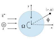
Figure 1: (Color online) Light scattering from a rotating dielectric cylinder.

Cylindrically Rotating Dielectric.– The exact electromagnetic constitutive equations in a medium moving at velocity $\mathbf{v}$, discovered by Minkowski Minkowski (1907), are

$$\mathbf{D}+\mathbf{v}\times\mathbf{H}/c = \epsilon\left(\mathbf{E}+\mathbf{v}\times\mathbf{B}/c\right)$$ (1)

$$\mathbf{B}+\mathbf{E}\times\mathbf{v}/c = \mu\left(\mathbf{H}+\mathbf{D}\times\mathbf{v}/c\right),$$ (2)

where $\mathbf{E}$, $\mathbf{D}$, $\mathbf{B}$ and $\mathbf{H}$ are the usual electromagnetic fields, $c$ is the speed of light in vacuum and $\epsilon$ is the electric permittivity in the rest frame and $\mu$ is the magnetic permeability in the rest frame. These equations presuppose uniform motion of the dielectric, where special relativity is sufficient. For accelerated dielectrics, the equations become more complicated; however, for rotating bodies with axial symmetry, the body in motion has the same shape as the one in the rest frame and it has been shown that the same equations would apply Sommerfeld ; Ridgely (1998); Tai . This assertion has been successfully used in applications Tai and was later proved rigorously by Ridgely Ridgely (1998), who showed that the general relativistic treatment for uniformly rotating dielectrics with axial-symmetry, to first order in $v/c$, gives Minkowski’s results (Eqs. 1 and 2).

In the limit where $v/c$ is small, Tai considered the scattered field of a plane wave incident upon a uniformly rotating dielectric cylinder with angular speed $\Omega$ Tai . We begin by reviewing Tai’s derivation of the scattered field and then we use these fields to compute the force. As depicted in Fig. 1, the velocity of the rotating body is $\mathbf{v}=\Omega r\mathbf{\hat{{\phi}}}$ at a radius $r$, the radius of the cylinder is denoted by $a$, and the $\mathbf{E}$ field of the incident wave is assumed to be polarized in the direction of the axis of the cylinder (which we take to be $\mathbf{\hat{z}}$).

Derivations of key equations are provided in the appendix.

We solve the scattering problem by standard technique of expanding the field in each region in basis of Bessel functions $J_{n}$ and then matching boundary conditions at the interface. In this basis, an incident $z$-polarized plane wave propagating in the $+x$ direction with amplitude $E_{0}$ (see Fig. 1) is given in polar $(r,\phi)$ coordinates by

$$E_{i}=E_{0}\mbox{exp}\left\{ik_{0}r\cos\phi\right\}=E_{0}\sum_{n=-\infty}^{+\infty}i^{n}J_{n}\left(k_{0}r\right)\mbox{exp}\left(in\phi\right),$$ (3)

where $E_{0}$ is the amplitude, $k_{0}=\omega/c$ is the wave number in vacuum, $\omega$ is the frequency in the time-harmonic oscillating field $e^{-i\omega t}$. The scattered and “transmitted” (interior) fields, respectively, can be written (using the Hankel function $H_{n}^{(1)}=J_{n}+iY_{n}$) with to-be-determined coefficients $\alpha_{n}$ and $\beta_{n}$:

$$E_{s} = E_{0}\sum_{n=-\infty}^{+\infty}\alpha_{n}i^{n}H_{n}^{\left(1\right)}\left(k_{0}r\right)\mbox{exp}\left(in\phi\right).$$ (4)

$$E_{t} = E_{0}\sum_{n=-\infty}^{+\infty}\beta_{n}i^{n}J_{n}\left(\gamma_{n}r\right)\mbox{exp}\left(in\phi\right),$$ (5)

where $\gamma_{n}$ is defined by

$$K \equiv \mu_{0}\left(\epsilon-\epsilon_{0}\right)\Omega$$ (6)

$$m \equiv 1-\frac{\epsilon_{0}}{\epsilon}$$ (7)

$$\gamma_{n}^{2} = k^{2}-2n\omega K=k^{2}\left(1-\frac{2nm\Omega}{\omega}\right).$$ (8)

The total field is therefore $\mathbf{E}=E_{z}\hat{\mathbf{z}}=\left(E_{i}+E_{s}\right)\hat{\mathbf{z}}$ and the magnetic field in the vacuum regions is given by $\mathbf{H}=\frac{1}{i\omega\mu_{0}}\nabla\times\mathbf{E}$.

The unknown coefficients $\beta_{n}$ and $\alpha_{n}$ are found by requiring continuity of $E_{z}$ and $H_{\phi}$ at $r=a$, yielding

$$J_{n}\left(k_{0}a\right)+\alpha_{n}H_{n}^{\left(1\right)}\left(k_{0}a\right) = \beta_{n}J_{n}\left(\gamma_{n}a\right)$$ (9)

$$k_{0}\left[J_{n}^{\prime}\left(k_{0}a\right)+\alpha_{n}H_{n}^{\left(1\right)}\left(k_{0}a\right)^{\prime}\right] = \beta_{n}\gamma_{n}J_{n}^{\prime}\left(\gamma_{n}a\right),$$ (10)

where the prime on $J$ and $H^{\left(1\right)}$ denotes derivative with respect to the entire argument. Solving for $\alpha_{n}$ gives

$$\alpha_{n}=-\frac{J_{n}\left(\rho_{0}\right)\left[J_{n-1}\left(\rho_{n}\right)-J_{n+1}\left(\rho_{n}\right)\right]-\frac{k_{0}}{\gamma_{n}}J_{n}\left(\rho_{n}\right)\left[J_{n-1}\left(\rho_{0}\right)-J_{n+1}\left(\rho_{0}\right)\right]}{H_{n}^{\left(1\right)}\left(\rho_{0}\right)\left[J_{n-1}\left(\rho_{n}\right)-J_{n+1}\left(\rho_{n}\right)\right]-\frac{k_{0}}{\gamma_{n}}J_{n}\left(\rho_{n}\right)\left[H_{n-1}^{\left(1\right)}\left(\rho_{0}\right)-H_{n+1}^{\left(1\right)}\left(\rho_{0}\right)\right]}.$$ (11)

where $\rho_{0}=k_{0}a$ and $\rho_{n}=\gamma_{n}a$. For $\Omega\neq 0$, the rotation breaks the $y=0$ mirror symmetry leading to asymmetrical scattering $\alpha_{n}\neq\alpha_{-n}$ as shown by Tai Tai . If $\Omega=0$, then $\alpha_{n}=\alpha_{-n}$ and Eq. 4 reduces to symmetrical scattering.

Force imparted to the Rotating Cylinder.– The asymmetry in the momentum transport by the scattered field should manifest itself as a lateral force on the dielectric. This force can be computed by integrating the Maxwell stress tensor over a closed surface around the object. Because we only evaluate the stress tensor in vacuum, we avoid the well-known difficulties that arise in defining the stress tensor inside the material Landau et al. (1984), nor does the rotation affect the vacuum stress tensor. The stress tensor in SI units is

$$\overleftrightarrow{\mathbf{\sigma}} = \epsilon_{0}\mathbf{E}\otimes\mathbf{E}+\mu_{0}\mathbf{H}\otimes\mathbf{H}$$

$$- \frac{1}{2}\left(\epsilon_{0}E^{2}+\mu_{0}H^{2}\right)\left(\mathbf{\hat{x}}\otimes\mathbf{\hat{x}}+\mathbf{\hat{y}}\otimes\mathbf{\hat{y}}+\mathbf{\hat{z}}\otimes\mathbf{\hat{z}}\right)$$

where the hatted quantities are unit vectors. To calculate the force on the cylinder in any direction $\hat{\mathbf{n_{0}}}$ on the plane at a fixed radius $r_{0}$, we evaluate

$$F_{\mathbf{\hat{n_{0}}}}=\frac{\omega}{2\pi}\int_{0}^{\frac{2\pi}{\omega}}dt\oint r\,dr\,d\phi\,\delta\left(r-r_{0}\right)\left\{\hat{\mathbf{n_{0}}}\cdot\overleftrightarrow{\mathbf{\sigma}}\cdot\hat{\mathbf{r}}\right\},$$ (13)

where $\hat{\mathbf{r}}=\cos\phi\mathbf{\hat{x}}+\sin\phi\mathbf{\hat{y}}$ and the time average is taken over a full period to obtain a real force. For our polarization, $E_{x}=E_{y}=H_{z}=0$. The force in $\hat{y}$ direction is

$$F_{\mathbf{\hat{y}}} = r_{0}\oint d\phi\left\{-\frac{\epsilon_{0}\left|E_{z}\right|^{2}+\mu_{0}\left|\mathbf{H}\right|^{2}}{4}\sin\phi\right.$$

$$+ \left.\frac{\mu_{0}}{2}\mbox{Re}\left(H_{x}^{*}H_{y}\right)\cos\phi+\frac{\mu_{0}\left|H_{y}\right|^{2}}{2}\sin\phi\right\}.$$

Using orthogonality conditions on $e^{in\phi}$, Eq. Optical “Bernoulli” forces can be integrated analytically. In the figures below we use the dimensionless force $\frac{F_{\mathbf{\hat{n_{0}}}}c}{P}$, where $P=2a\left|E_{0}\right|^{2}\sqrt{\frac{\epsilon_{0}}{\mu_{0}}}$ is the incident power on the scatterer’s geometric cross section. This is a convenient normalization because, for light incident on a perfectly absorbing flat surface the force is exactly $\frac{P}{c}$, so this normalization gives a measure of the lateral force relative to the incident photon pressure. Furthermore, we use the dimensionless angular frequency $\frac{a\Omega}{c}$, which is the ratio of speed of the cylinder boundary to that of light.

Fig. 2 plots the force vs. angular frequency for $\epsilon/\epsilon_{0}=10$. As discussed below, whenever $\epsilon>\epsilon_{0}$, corresponding to a positive electric susceptibility $\chi^{(\mbox{e})}=\epsilon/\epsilon_{0}-1$, there is a force of sign analogous to Bernoulli’s law, where $\Omega>0$ (counterclockwise rotation) gives a force in the positive $y$ direction. Clearly, $\Omega<0$ gives the same magnitude of the force in the opposite direction as expected from the symmetry of the problem and in accordance with the fluid-mechanical analogy.

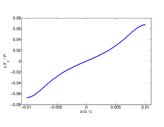
Figure 2: (Color online) Normalized force vs. rotational frequency for $\lambda_{0}=0.01$ and $\epsilon/\epsilon_{0}=10$ where $P=2a\left|E_{0}\right|^{2}\sqrt{\frac{\epsilon_{0}}{\mu_{0}}}$.

In the case of a perfect conductor, $\beta_{n}$ is zero (see Eq. 5) and therefore Eqs. 9 and 10 do not give an asymmetry with respect to $n$ for $\alpha_{n}$. Consequently, in this limit there is no lateral force. Intuitively, because a perfect conductor allows no penetration of the electromagnetic fields, the fields cannot “notice” that it is rotating or be “dragged” by the moving matter. However, for imperfect metals (finite $\epsilon<0$) there is some penetration of the radiation into the material which results in a lateral force. Interestingly, in the case of $\epsilon<0$, and in fact whenever $\epsilon<\epsilon_{0}$ (negative susceptibility), the force is in the opposite direction of the force for $\epsilon>\epsilon_{0}$ dielectrics (see Fig. 3). The reason is an immediate consequence of Eq. 6. For $\epsilon<\epsilon_{0}$ and $\Omega>0$, $K$ becomes negative and the phenomenology, looking at $\gamma_{n}$ in Eq. 8, become equivalent to the case of $\epsilon>\epsilon_{0}$ and $\Omega<0$. The same relationship between the sign of the force and the sign of $\operatorname{Re}\epsilon-\epsilon_{0}$ holds for complex $\epsilon$ as long as $|\operatorname{Im}\epsilon|\ll|\operatorname{Re}\epsilon|$, whereas for large $|\operatorname{Im}\epsilon|$ we observe a similar relationship with the sign of the imaginary part.

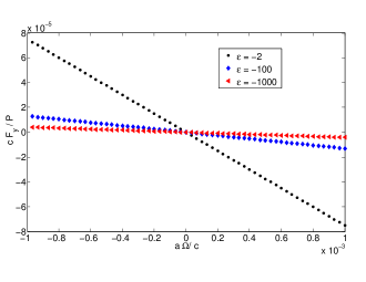
Figure 3: (Color online) Normalized Force vs. Rotational frequency for $\lambda_{0}=0.01$ and various $\epsilon/\epsilon_{0}$ where $P=2a\left|E_{0}\right|^{2}\sqrt{\frac{\epsilon_{0}}{\mu_{0}}}$.

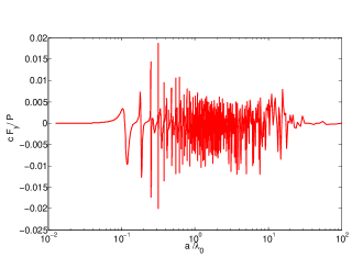
Figure 4: (Color online) Mie resonances: Normalized force vs. $\lambda_{0}$ for $a\Omega/c=3.34e-4$ and $a=0.01$.

Lastly, we investigate the dependence of the normalized force on $2\pi\omega a/c=a/\lambda_{0}$, varying the vacuum wavelength $\lambda_{0}$ (see Fig. 4). For $\lambda_{0}\ll a$ the scattering approaches a ray-optics limit, while for $\lambda_{0}\gg a$ it is in the Rayleigh-scattering (dipole approximation) regime Jackson (1998). For $\lambda_{0}\sim a$, the force spectrum becomes more interesting due to the presence of Mie resonances Stratton (1941).

Discussion and Future Work.– Given a finite amount of power, one would use a focused beam rather than a plane-wave, and an interesting question for future work is what beam width (and profile) maximizes the lateral force for a given total power; we conjecture that the optimal beam width should be comparable to the scattering cross-section.

Furthermore, recent work has shown that an appropriate beam can form an optical "tweezers" Ashkin et al. (1986) or "tractor beam" in which the sign of the longitudinal force on a non-spinning particle can reverse Chen et al. (2011); Lee et al. (2010); Marston (2006). Applied to a spinning particle, the ability to change the sign of the longitudinal force implies that there should also be a zero point: a beam for which the force of is purely lateral.

The forces obtained here are only a fraction of the incident radiation pressure and seem to require infeasible rotation rates, but we expect that they can be resonantly enhanced by techniques similar to those that have been used by other authors to enhance scattered power for a given particle diameter. Mie resonances are already visible in Fig. 4, but much stronger resonant phenomena can be designed by using multilayer spheres that trap light using Bragg mirrors and/or specially designed surface plasmons, and one can even obtain “superscattering” by aligning multiple resonances at the same frequency Ruan and Fan (2011).

Material dispersion will contribute an additional source of lateral force: similar to the origin of quantum friction  Zhao et al. (2012); Manjavacas and GarciadeAbajo (2010); Pendry (2010), the Doppler shift in the material dispersion should differ between the sides of the object moving toward and away from the light source, causing additional asymmetry in the scattered field and hence additional lateral force.

Such enhancement mechanism, in combination with recent progress in generating rotating particles (of graphene) at near-GHz $\Omega$ Kane (2010), may permit the future experimental observation and exploitation of optical “Bernoulli” forces.

SGJ was supported in part by the U.S. Army Research Office under contract W911NF-13-D-0001.

I Appendix

First let $\sigma,\mu,\epsilon$ be the conductivity, permeability and permittivity respectively and define $\mathbf{\Lambda}=\left(\epsilon\mu-\epsilon_{0}\mu_{0}\right)\mathbf{v}$, where subscript $0$ corresponds to quantities in the vacuum. The electric and magnetic field vectors satisfy

$$\nabla\times\mathbf{E} = -\frac{\partial}{\partial t}\left(\mu\mathbf{H-\Lambda}\times\mathbf{E}\right)$$ (15)

$$\nabla\times\mathbf{H} = \sigma\left(\mathbf{E}+\mu\mathbf{v}\times\mathbf{H}\right)+\frac{\partial}{\partial t}\left(\sigma\mathbf{E+\Lambda}\times\mathbf{H}\right).$$ (16)

To determine the proper expression for the transmitted wave, we use harmonically oscillating fields to reduce Eqs. 15 and 16 to (neglecting $\mathcal{O}\left(\left(v/c\right)^{2}\right)$ terms)

$$\left(\nabla+i\omega\mathbf{\Lambda}\right)\times\mathbf{E} = i\omega\mu\mathbf{H}$$ (17)

$$\left(\nabla+i\omega\mathbf{\Lambda}-\sigma\mu\mathbf{v}\right)\times\mathbf{H} = \left(\sigma-i\omega\epsilon\right)\mathbf{E}$$ (18)

Looking at Figure 1, the incident wave is given by

$$E_{i}=E_{0}\mbox{exp}\left\{ik_{0}r\cos\phi\right\}=E_{0}\sum_{n=-\infty}^{+\infty}i^{n}J_{n}\left(k_{0}r\right)\mbox{exp}\left(in\phi\right),$$ (19)

where $k_{0}=\omega/c$ is the wave number in vacuo; $\omega$ being the frequency in the time harmonic oscillating field $e^{i\omega t}$. The scattering field can be written in the form

$$E_{s}=E_{0}\sum_{n=-\infty}^{+\infty}\alpha_{n}i^{n}H_{n}^{\left(1\right)}\left(k_{0}r\right)\mbox{exp}\left(in\phi\right).$$ (20)

To solve for the transmitted field inside the dielectric we subject Eqs. 17 and 18 to the particular form of the velocity which is independent of $\mathbf{\hat{z}}$. The parameter $\mathbf{\Lambda}$ is then a function of $r$ alone,

$$\mathbf{\Lambda=}\mu_{0}\left(\epsilon-\epsilon_{0}\right)\mathbf{v}=Kr\mathbf{\hat{\mathbf{\phi}}}$$ (21)

where $K\equiv\mu_{0}\epsilon\left(1-\frac{\epsilon_{0}}{\epsilon}\right)\Omega=\frac{m\Omega}{c^{2}}$, with $m\equiv 1-\frac{\epsilon_{0}}{\epsilon}$ and $c^{2}=1/\mu_{0}\epsilon$. Substituting Eq. 21 into Eqs. 17 and 18 and eliminating $\mathbf{H}$ we obtain a differential equation for $E_{z}$ which is the only component of the electric field inside the dielectric cylinder.

$$\frac{1}{r}\frac{\partial}{\partial r}\left(r\frac{\partial E_{z}}{\partial r}\right)+\frac{1}{r^{2}}\frac{\partial^{2}E_{z}}{\partial\phi^{2}}+2i\omega K\frac{\partial E_{z}}{\partial\phi}+k^{2}E_{z}+\mathcal{O}\left(\left(\frac{v}{c}\right)^{2}\right)=0,$$ (22)

where $k^{2}=\left(\omega/c\right)^{2}$. To solve let us seek separable solutions for $E_{z}=F\left(r\right)e^{in\phi}$ and below we drop $\mathcal{O}\left(\left(\frac{v}{c}\right)^{2}\right)$ by understanding that the results are accurate to first order. The function $F\left(r\right)$ then satisfies

$$\frac{1}{r}\frac{\partial}{\partial r}\left(r\frac{\partial F}{\partial r}\right)-\left(\frac{n^{2}}{r^{2}}+2n\omega K-k^{2}\right)F=0.$$

If we introduce $\gamma_{n}^{2}=k^{2}-2n\omega K=k^{2}\left(1-\frac{2nm\Omega}{\omega}\right),$ then the proper set of radial functions to describe the field inside the rotating cylinder is

$$F\left(r\right)=J_{n}\left(\gamma_{n}r\right),\qquad n=0,\pm 1,\pm 2,\cdots.$$

The complete expression for the transmitted field can be written in the form

$$E_{t}=E_{0}\sum_{n=-\infty}^{+\infty}\beta_{n}i^{n}J_{n}\left(\gamma_{n}r\right)\mbox{exp}\left(in\phi\right).$$ (23)

By matching $E_{z}$ as defined by Eqs. 19, 20 and 23, and the $\phi-$component of the magnetic field at the boundary $r=a$ one obtains the following two simultaneous equations:

$$J_{n}\left(k_{0}a\right)+\alpha_{n}H_{n}^{\left(1\right)}\left(k_{0}a\right) = \beta_{n}J_{n}\left(\gamma_{n}a\right)$$ (24)

$$k_{0}\left[J_{n}^{\prime}\left(k_{0}a\right)+\alpha_{n}H_{n}^{\left(1\right)}\left(k_{0}a\right)^{\prime}\right] = \beta_{n}\gamma_{n}J_{n}^{\prime}\left(\gamma_{n}a\right),$$ (25)

where the prime on $J$ and $H^{\left(1\right)}$ denotes derivative with respect to the entire argument of these functions. The solutions for $\alpha_{n}$ and $\beta_{n}$ are

$$\alpha_{n} = -\frac{J_{n}\left(\rho_{0}\right)J^{\prime}_{n}\left(\rho_{n}\right)-\frac{k_{0}}{\gamma_{n}}J_{n}\left(\rho_{n}\right)J^{\prime}_{n}\left(\rho_{0}\right)}{H_{n}^{\left(1\right)}\left(\rho_{0}\right)J^{\prime}_{n}\left(\rho_{n}\right)-\frac{k_{0}}{\gamma_{n}}J_{n}\left(\rho_{n}\right)H_{n}^{\left(1\right)}\mbox{}^{\prime}\left(\rho_{0}\right)}$$ (26)

$$\beta_{n} = -\frac{k_{0}}{\gamma_{n}}\frac{\left[J_{n}\left(\rho_{0}\right)H_{n}^{\left(1\right)}\mbox{}^{\prime}\left(\rho_{0}\right)-J_{n}^{\prime}\left(\rho_{0}\right)H_{n}^{\left(1\right)}\left(\rho_{0}\right)\right]}{H_{n}^{\left(1\right)}\left(\rho_{0}\right)J^{\prime}_{n}\left(\rho_{n}\right)-\frac{k_{0}}{\gamma_{n}}J_{n}\left(\rho_{n}\right)H_{n}^{\left(1\right)}\mbox{}^{\prime}\left(\rho_{0}\right)},$$ (27)

where $\rho_{0}=k_{0}a$ and $\rho_{n}=\gamma_{n}a$. Using identities $J^{\prime}_{n}\left(x\right)=\frac{1}{2}\left[J_{n-1}\left(x\right)-J_{n+1}\left(x\right)\right]$, $J^{\prime}_{0}\left(x\right)=-J_{1}\left(x\right)$ and $H_{n}^{\left(1\right)}\mbox{}^{\prime}\left(x\right)=\frac{1}{2}\left[H_{n-1}^{\left(1\right)}\left(x\right)-H_{n+1}^{\left(1\right)}\left(x\right)\right]$, $H_{0}^{\left(1\right)}\mbox{}^{\prime}\left(x\right)=-H_{1}^{\left(1\right)}\left(x\right)$, $\beta_{n}$ can be eliminated to give

$$\alpha_{n}=-\frac{J_{n}\left(\rho_{0}\right)\left[J_{n-1}\left(\rho_{n}\right)-J_{n+1}\left(\rho_{n}\right)\right]-\frac{k_{0}}{\gamma_{n}}J_{n}\left(\rho_{n}\right)\left[J_{n-1}\left(\rho_{0}\right)-J_{n+1}\left(\rho_{0}\right)\right]}{H_{n}^{\left(1\right)}\left(\rho_{0}\right)\left[J_{n-1}\left(\rho_{n}\right)-J_{n+1}\left(\rho_{n}\right)\right]-\frac{k_{0}}{\gamma_{n}}J_{n}\left(\rho_{n}\right)\left[H_{n-1}^{\left(1\right)}\left(\rho_{0}\right)-H_{n+1}^{\left(1\right)}\left(\rho_{0}\right)\right]}.$$ (28)

The numerical value of $\alpha_{n}\neq\alpha_{-n}$ for $\Omega\neq 0$ because in this case $\rho_{n}\neq\rho_{-n}$ and $\gamma_{n}\neq\gamma_{-n}$ hence the scattering field has an asymmetrical part with respect to the direction of incidence, $\phi=0$. When $\Omega=0\implies\alpha_{n}=\alpha_{-n}$ and Eq. 20 reduces to the well known results.

The total field therefore is $\mathbf{E}=E_{z}\hat{\mathbf{z}}=\left(E_{i}+E_{s}\right)\hat{\mathbf{z}}$. Below we suppress $k_{0}r$ as the argument of the Bessel functions unless stated otherwise.

$$E_{z}=E_{0}\sum_{n=-\infty}^{+\infty}i^{n}\left\{J_{n}+\alpha_{n}H_{n}^{\left(1\right)}\right\}e^{in\phi}$$ (29)

Further in free space we have $\mathbf{H}=\frac{1}{i\omega\mu_{0}}\nabla\times\mathbf{E}$ which gives

$$\mathbf{H} = \frac{1}{i\omega\mu_{0}}\nabla\times E\hat{\mathbf{z}}=\frac{1}{i\omega\mu_{0}}\left(\frac{1}{r}\frac{\partial E_{z}}{\partial\phi}\hat{\mathbf{r}}-\frac{\partial E_{z}}{\partial r}\hat{\mathbf{\phi}}\right)$$

$$= \frac{1}{i\omega\mu_{0}}\left(\frac{1}{r}\frac{\partial E_{z}}{\partial\phi}\cos\phi+\frac{\partial E_{z}}{\partial r}\sin\phi\right)\hat{\mathbf{x}}$$

$$+ \frac{1}{i\omega\mu_{0}}\left(\frac{1}{r}\frac{\partial E_{z}}{\partial\phi}\sin\phi-\frac{\partial E_{z}}{\partial r}\cos\phi\right)\hat{\mathbf{y}}.$$

Let $\mathbf{\hat{n_{0}}=}\cos\psi\mathbf{\hat{x}}+\sin\psi\mathbf{\hat{y}}$ be any unit vector, then Eq. Optical “Bernoulli” forces, evaluated at the radius $r_{0}$, reads

$$F_{\mathbf{\hat{n_{0}}}} = r_{0}\oint d\phi\left\{-\frac{\epsilon_{0}\left|E\right|^{2}+\mu_{0}\left|H\right|^{2}}{4}\cos\left(\psi-\phi\right)\right.$$

$$+ \frac{\mu_{0}}{2}\mbox{Re}\left(H_{x}^{*}H_{y}\right)\sin\left(\psi+\phi\right)$$

$$+ \left.\frac{\mu_{0}\left|H_{x}\right|^{2}}{2}\cos\phi\cos\psi+\frac{\mu_{0}\left|H_{y}\right|^{2}}{2}\sin\phi\sin\psi\right\}.$$

In particular we are interested in $\psi=\frac{\pi}{2}$ to calculate the transverse force

$$F_{\mathbf{\hat{y}}} = r_{0}\oint d\phi\left\{-\frac{\epsilon_{0}\left|E\right|^{2}+\mu_{0}\left|H\right|^{2}}{4}\sin\phi\right.$$ (32)

$$+ \left.\frac{\mu_{0}}{2}\mbox{Re}\left(H_{x}^{*}H_{y}\right)\cos\phi+\frac{\mu_{0}\left|H_{y}\right|^{2}}{2}\sin\phi\right\}.$$ (33)

where $E=\left(E_{i}+E_{s}\right)$ is given by Eqs. 3 and 4.

II Evaluating the Integral

Here we evaluate $\left|E\right|^{2}$, $\left|H\right|^{2}$, $\left|H_{y}^{2}\right|$ and $\mbox{Re}\left(H_{x}^{*}H_{y}\right)$ as they are useful for calculating the force below (Eqs. I and Optical “Bernoulli” forces). The key equations are

$$E_{z} = E_{0}\sum_{n=-\infty}^{+\infty}i^{n}\left\{J_{n}+\alpha_{n}H_{n}^{\left(1\right)}\right\}e^{in\phi}$$

$$\mathbf{H} \equiv H_{x}\hat{\mathbf{x}}+H_{y}\hat{\mathbf{y}}$$

$$= \frac{1}{i\omega\mu_{0}}\left(\frac{1}{r}\frac{\partial E_{z}}{\partial\phi}\cos\phi+\frac{\partial E_{z}}{\partial r}\sin\phi\right)\hat{\mathbf{x}}$$

$$+ \frac{1}{i\omega\mu_{0}}\left(\frac{1}{r}\frac{\partial E_{z}}{\partial\phi}\sin\phi-\frac{\partial E_{z}}{\partial r}\cos\phi\right)\hat{\mathbf{y}}.$$

where

$$H_{x} = \frac{E_{0}}{i\omega\mu_{0}}\sum_{n=-\infty}^{+\infty}e^{in\phi}i^{n}\left\{\frac{in}{r}\left[J_{n}+\alpha_{n}H_{n}^{\left(1\right)}\right]\cos\phi+\frac{k_{0}}{2}\left[J_{n-1}-J_{n+1}+\alpha_{n}\left(H_{n-1}^{\left(1\right)}-H_{n+1}^{\left(1\right)}\right)\right]\sin\phi\right\}$$

$$H_{y} = \frac{E_{0}}{i\omega\mu_{0}}\sum_{n=-\infty}^{+\infty}e^{in\phi}i^{n}\left\{\frac{in}{r}\left[J_{n}+\alpha_{n}H_{n}^{\left(1\right)}\right]\sin\phi-\frac{k_{0}}{2}\left[J_{n-1}-J_{n+1}+\alpha_{n}\left(H_{n-1}^{\left(1\right)}-H_{n+1}^{\left(1\right)}\right)\right]\cos\phi\right\}$$

as well as the orthogonality relations

$$\oint d\phi e^{i\left(n-m\right)\phi}\sin\phi = \left(-i\pi\right)\left(\delta_{n,m-1}-\delta_{n,m+1}\right)$$

$$\oint d\phi e^{i\left(n-m\right)\phi}\sin^{3}\phi = \left(\frac{i\pi}{4}\right)\left(\delta_{n,m-3}-\delta_{n,m+3}-3\delta_{n,m-1}+3\delta_{n,m+1}\right)$$

$$\oint d\phi e^{i\left(n-m\right)\phi}\sin^{2}\phi\cos\phi = \left(\frac{-\pi}{4}\right)\left(\delta_{n,m-3}+\delta_{n,m+3}-\delta_{n,m-1}-\delta_{n,m+1}\right)$$

$$\oint d\phi e^{i\left(n-m\right)\phi}\sin\phi\cos^{2}\phi = \left(\frac{-i\pi}{4}\right)\left(\delta_{n,m-3}-\delta_{n,m+3}+\delta_{n,m-1}-\delta_{n,m+1}\right)$$

$$\oint d\phi e^{i\left(n-m\right)\phi}\cos^{3}\phi = \left(\frac{\pi}{4}\right)\left(\delta_{n,m-3}+\delta_{n,m+3}+3\delta_{n,m-1}+3\delta_{n,m+1}\right).$$

We proceed

$$\oint d\phi\left|E_{z}\right|^{2}\sin\phi = E_{0}^{2}\sum_{n,m=-\infty}^{+\infty}\oint d\phi e^{i\left(n-m\right)\phi}\sin\phi\left(-1\right)^{m}i^{n+m}\left\{J_{n}+\alpha_{n}H_{n}^{\left(1\right)}\right\}\left\{J_{m}+\alpha_{m}^{*}H_{m}^{\left(2\right)}\right\}$$

$$= E_{0}^{2}\sum_{n,m=-\infty}^{+\infty}\left(-1\right)^{m}i^{n+m}\left\{J_{n}+\alpha_{n}H_{n}^{\left(1\right)}\right\}\left\{J_{m}+\alpha_{m}^{*}H_{m}^{\left(2\right)}\right\}\left(-i\pi\right)\left\{\delta_{n,m-1}-\delta_{n,m+1}\right\}$$

Further $\oint d\phi\left|H_{x}\right|^{2}\sin\phi=\oint d\phi\left(H_{x}^{*}H_{x}\right)\sin\phi$, similarly for $\oint d\phi\left|H_{y}\right|^{2}\sin\phi$

$$\oint d\phi\left|H_{x}\right|^{2}\sin\phi = \left(\frac{E_{0}}{\omega\mu_{0}}\right)^{2}\sum_{n,m=-\infty}^{+\infty}\left(-1\right)^{m}i^{n+m}\oint d\phi\sin\phi e^{i\left(n-m\right)\phi}$$

$$\left\{\left(\frac{-im}{r}\left[J_{m}+\alpha_{m}^{*}H_{m}^{\left(2\right)}\right]\cos\phi+\frac{k_{0}}{2}\left[J_{m-1}-J_{m+1}+\alpha_{m}^{*}\left(H_{m-1}^{\left(2\right)}-H_{m+1}^{\left(2\right)}\right)\right]\sin\phi\right)\right.$$

$$\times \left.\left(\frac{in}{r}\left[J_{n}+\alpha_{n}H_{n}^{\left(1\right)}\right]\cos\phi+\frac{k_{0}}{2}\left[J_{n-1}-J_{n+1}+\alpha_{n}\left(H_{n-1}^{\left(1\right)}-H_{n+1}^{\left(1\right)}\right)\right]\sin\phi\right)\right\}$$

which using the orthogonality relations yields

$$\oint d\phi\left|H_{x}\right|^{2}\sin\phi = \left(\frac{E_{0}}{\omega\mu_{0}}\right)^{2}\sum_{n,m=-\infty}^{+\infty}\left(-1\right)^{m}i^{n+m}$$

$$\frac{nm}{r^{2}}\left(J_{m}+\alpha_{m}^{*}H_{m}^{\left(2\right)}\right)\left(J_{n}+\alpha_{n}H_{n}^{\left(1\right)}\right)\left(\frac{-i\pi}{4}\right)\left(\delta_{n,m-3}-\delta_{n,m+3}+\delta_{n,m-1}-\delta_{n,m+1}\right)$$

$$+ \frac{k_{0}^{2}}{4}\left[J_{m-1}-J_{m+1}+\alpha_{m}^{*}\left(H_{m-1}^{\left(2\right)}-H_{m+1}^{\left(2\right)}\right)\right]\left[J_{n-1}-J_{n+1}+\alpha_{n}\left(H_{n-1}^{\left(1\right)}-H_{n+1}^{\left(1\right)}\right)\right]$$

$$\times \left(\frac{i\pi}{4}\right)\left(\delta_{n,m-3}-\delta_{n,m+3}-3\delta_{n,m-1}+3\delta_{n,m+1}\right)$$

$$+ \frac{ik_{0}}{2r}\left[-m\left(J_{m}+\alpha_{m}^{*}H_{m}^{\left(2\right)}\right)\left(J_{n-1}-J_{n+1}+\alpha_{n}\left(H_{n-1}^{\left(1\right)}-H_{n+1}^{\left(1\right)}\right)\right)\right.$$

$$\;\left.+n\left(J_{n}+\alpha_{n}H_{n}^{\left(1\right)}\right)\left(J_{m-1}-J_{m+1}+\alpha_{m}^{*}\left(H_{m-1}^{\left(2\right)}-H_{m+1}^{\left(2\right)}\right)\right)\right]$$

$$\times \left(\frac{-\pi}{4}\right)\left(\delta_{n,m-3}+\delta_{n,m+3}-\delta_{n,m-1}-\delta_{n,m+1}\right)$$

Similarly

$$\oint d\phi\left|H_{y}\right|^{2}\sin\phi = \left(\frac{E_{0}}{\omega\mu_{0}}\right)^{2}\sum_{n,m=-\infty}^{+\infty}\left(-1\right)^{m}i^{n+m}\oint d\phi\sin\phi e^{i\left(n-m\right)\phi}$$

$$\left\{\left(\frac{-im}{r}\left[J_{m}+\alpha_{m}^{*}H_{m}^{\left(2\right)}\right]\sin\phi-\frac{k_{0}}{2}\left[J_{m-1}-J_{m+1}+\alpha_{m}^{*}\left(H_{m-1}^{\left(2\right)}-H_{m+1}^{\left(2\right)}\right)\right]\cos\phi\right)\right.$$

$$\times \left.\left(\frac{in}{r}\left[J_{n}+\alpha_{n}H_{n}^{\left(1\right)}\right]\sin\phi-\frac{k_{0}}{2}\left[J_{n-1}-J_{n+1}+\alpha_{n}\left(H_{n-1}^{\left(1\right)}-H_{n+1}^{\left(1\right)}\right)\right]\cos\phi\right)\right\}$$

which using the orthogonality relations yields

$$\oint d\phi\left|H_{y}\right|^{2}\sin\phi = \left(\frac{E_{0}}{\omega\mu_{0}}\right)^{2}\sum_{n,m=-\infty}^{+\infty}\left(-1\right)^{m}i^{n+m}$$

$$\frac{mn}{r^{2}}\left(J_{n}+\alpha_{n}H_{n}^{\left(1\right)}\right)\left(J_{m}+\alpha_{m}^{*}H_{m}^{\left(2\right)}\right)\left(\frac{i\pi}{4}\right)\left(\delta_{n,m-3}-\delta_{n,m+3}-3\delta_{n,m-1}+3\delta_{n,m+1}\right)$$

$$+ \frac{k_{0}^{2}}{4}\left(J_{m-1}-J_{m+1}+\alpha_{m}^{*}\left(H_{m-1}^{\left(2\right)}-H_{m+1}^{\left(2\right)}\right)\right)\left(J_{n-1}-J_{n+1}+\alpha_{n}\left(H_{n-1}^{\left(1\right)}-H_{n+1}^{\left(1\right)}\right)\right)$$

$$\times \left(\frac{-i\pi}{4}\right)\left(\delta_{n,m-3}-\delta_{n,m+3}+\delta_{n,m-1}-\delta_{n,m+1}\right)$$

$$+ \frac{ik_{0}}{2r}\left[m\left(J_{m}+\alpha_{m}^{*}H_{m}^{\left(2\right)}\right)\left(J_{n-1}-J_{n+1}+\alpha_{n}\left(H_{n-1}^{\left(1\right)}-H_{n+1}^{\left(1\right)}\right)\right)\right.$$

$$\;\left.-n\left(J_{n}+\alpha_{n}H_{n}^{\left(1\right)}\right)\left(J_{m-1}-J_{m+1}+\alpha_{m}^{*}\left(H_{m-1}^{\left(2\right)}-H_{m+1}^{\left(2\right)}\right)\right)\right]$$

$$\times \left(\frac{-\pi}{4}\right)\left(\delta_{n,m-3}+\delta_{n,m+3}-\delta_{n,m-1}-\delta_{n,m+1}\right).$$

Lastly we need $\oint d\phi\mbox{Re}\left(H_{x}^{*}H_{y}\right)\cos\phi=\frac{1}{2}\oint d\phi H_{x}^{*}H_{y}\cos\phi+c.c.$

$$\oint d\phi H_{x}^{*}H_{y}\cos\phi = \left(\frac{E_{0}}{\omega\mu_{0}}\right)^{2}\sum_{n,m=-\infty}^{+\infty}\left(-1\right)^{m}i^{n+m}\oint d\phi\cos\phi e^{i\left(n-m\right)\phi}$$

$$\left\{\left(\frac{-im}{r}\left[J_{m}+\alpha_{m}^{*}H_{m}^{\left(2\right)}\right]\cos\phi+\frac{k_{0}}{2}\left[J_{m-1}-J_{m+1}+\alpha_{m}^{*}\left(H_{m-1}^{\left(2\right)}-H_{m+1}^{\left(2\right)}\right)\right]\sin\phi\right)\right.$$

$$\times \left.\left(\frac{in}{r}\left[J_{n}+\alpha_{n}H_{n}^{\left(1\right)}\right]\sin\phi-\frac{k_{0}}{2}\left[J_{n-1}-J_{n+1}+\alpha_{n}\left(H_{n-1}^{\left(1\right)}-H_{n+1}^{\left(1\right)}\right)\right]\cos\phi\right)\right\}$$

which using the orthogonality relations yields

$$\oint d\phi H_{x}^{*}H_{y}\cos\phi = \left(\frac{E_{0}}{\omega\mu_{0}}\right)^{2}\sum_{n,m=-\infty}^{+\infty}\left(-1\right)^{m}i^{n+m}$$

$$\left[\frac{mn}{r^{2}}\left(J_{m}+\alpha_{m}^{*}H_{m}^{\left(2\right)}\right)\left(J_{n}+\alpha_{n}H_{n}^{\left(1\right)}\right)-\frac{k_{0}^{2}}{4}\left(J_{m-1}-J_{m+1}+\alpha_{m}^{*}\left(H_{m-1}^{\left(2\right)}-H_{m+1}^{\left(2\right)}\right)\right)\right.$$

$$\left.\times\left(J_{n-1}-J_{n+1}+\alpha_{n}\left(H_{n-1}^{\left(1\right)}-H_{n+1}^{\left(1\right)}\right)\right)\left(-\frac{i\pi}{4}\right)\right]\left(\delta_{n,m-3}-\delta_{n,m+3}+\delta_{n,m-1}-\delta_{n,m+1}\right)$$

$$+ \frac{imk_{0}}{2r}\left(J_{m}+\alpha_{m}^{*}H_{m}^{\left(2\right)}\right)\left(J_{n-1}-J_{n+1}+\alpha_{n}\left(H_{n-1}^{\left(1\right)}-H_{n+1}^{\left(1\right)}\right)\right)$$

$$\times\left(\frac{\pi}{4}\right)\left(\delta_{n,m-3}+\delta_{n,m+3}+3\delta_{n,m-1}+3\delta_{n,m+1}\right)$$

$$+ \frac{ink_{0}}{2r}\left(J_{n}+\alpha_{n}H_{n}^{\left(1\right)}\right)\left(J_{m-1}-J_{m+1}+\alpha_{m}^{*}\left(H_{m-1}^{\left(2\right)}-H_{m+1}^{\left(2\right)}\right)\right)$$

$$\times\left(\frac{-\pi}{4}\right)\left(\delta_{n,m-3}+\delta_{n,m+3}-\delta_{n,m-1}-\delta_{n,m+1}\right).$$

All of the above integrals were checked against numerics before calculating the cumulative effect that appears in the force Eq. Optical “Bernoulli” forces. The total force was also checked against numerical experiments. In all cases agreements were found with errors of order $\mathcal{O}\left(10^{-26}\right)$.

References

Möller (1957)C. Möller, The Theory of
Relativity (Oxford University Press, 1957).
(2)C. T. Tai, Ohio State Univ., Res.
Foundation, Rep., 1691.
Minkowski (1907) H. Minkowski, von der Gesellschaft der Wissenschaften zu Göttingen,
Mathematisch-Physikalische Klasse, 53, 111 (1907).
(4)A. Sommerfeld, Electrodynamics’ (Academic Press, New York).
Ridgely (1998)C. T. Ridgely, Am.
J. Phys., 66 (1998).
Landau et al. (1984)L. D. Landau, E. Lifshitz, and L. Pitaevskii, ‘Electrodynamics of Continuous
Media (Pergamon Press, 1984).
Jackson (1998)J. D. Jackson, Classical
Electrodynamics (Third Edition, Wiley, 1998).
Stratton (1941)J. A. Stratton, Electromagnetic
Theory (New York: McGraw-Hill, 1941).
Ashkin et al. (1986)A. Ashkin, J. M. Dziedzic, J. E. Bjorkholm, , and S. Chu, Optics
Letters, 11, 288
(1986).
Chen et al. (2011)J. Chen, J. Ng, Z. Lin, and C. T. Chan, Nature Photonics, 5, 531 (2011).
Lee et al. (2010)S.-H. Lee, Y. Roichman, and D. G. Grier, Optics Express, 18, 6988 (2010).
Marston (2006)P. L. Marston, J.
Acoust. Soc. Am., 120, 3518 (2006).
Ruan and Fan (2011)Z. Ruan and S. Fan, Appl. Phys.
Lett., 98, 043101
(2011).
Zhao et al. (2012)R. Zhao, A. Manjavacas,
F. J. GarciadeAbajo, and J. B. Pendry, Phys. Rev.
Lett., 109, 123604
(2012).
Manjavacas and GarciadeAbajo (2010)A. Manjavacas and F. J. GarciadeAbajo, Phys. Rev. A, 82, 063827 (2010).
Pendry (2010)J. B. Pendry, New J.
Phys., 12, 033028
(2010).
Kane (2010)B. E. Kane, Physical
Review B, 82, 115441
(2010).