On the multifractal structure of fully developed turbulence.

Abstract

The appearance of vortex filaments, the power-law dependence of velocity and vorticity correlators and their multiscaling behavior are derived from the Navier-Stokes equation. This is possible due to interpretation of the Navier-Stokes equation as an equation with multiplicative noise, and remarkable properties of random matrix products.

I Introduction

Understanding of statistical properties of a turbulent flow is a classical problem of hydrodynamics. Intermittent behavior of velocity scaling exponents demonstrated in experiments and numerical simulations observations ; simulations ; arneodo is one of its important aspects. The most successful, and conventional nowadays, way to interpret this intermittency is the Multifractal (MF) approach introduced in ParisiFrisch . This is a generalization of Kolmogorov’s K41 theory, and it allows to express all the observed intermittent characteristics by means of one function $D(h)$. In particular, if $D(h)$ is derived from observed velocity scaling exponents, then all the other values can be calculated 25years .

However, the phenomenological presentation of the MF model assumes the existence of singularities (actually, the paper ParisiFrisch was titled ’On the singularity structure of fully developed turbulence’). The question if singularities can appear after a finite time has been widely discussed and remains still open Frisch ; Kuznetsov ; Kuznetsov2 . But in the absence of even one example of a finite-time singularity, the existence of a whole ’spectrum’ of singularities is rather doubtful.

To make the MF theory independent of this assumption, its probabilistic reformulation was introduced Frisch ; MeneveauSreeni91 ; Mandelbrot91 . However, this formulation does not allow to understand what happens in a turbulent flow; the structures (or the solutions to the Navier-Stokes equation) that are responsible for the observed intermittent properties, remain unknown.

On the other hand, many experiments and numerical simulations have shown the presence of ’coherent structures’ - vortex filaments and ’pancakes’ - in a turbulent flow (see, e.g., Frisch208vnizu or others? ). In Farge it was shown that these structures make a fundamental contribution to the observed Kolmogorov’s two-thirds law, and they contain the most part of the whole enstrophy of a flow. The origin of these coherent structures is still obscure (in Frisch the tendency of a flow to produce these structures was characterized as ’mysterious’). Understanding of these filaments formation seems to be very important as it may also help to understand the cause of intermittency and multifractality.

In our previous papers we have developed a model of vortex filaments (VF). We showed that it did not contradict to the MF model PhysicaD . In PRE2 ; notPRE ; Scripta13 we combined the VF theory with the MF approach; this allowed to calculate both longitudinal and transverse velocity scaling exponents without adjusting parameters, the result agreed well with numerical data. Although this model was based on the Navier-Stokes equation (NSE), it still contained an additional supposition: it assumed that the nonlinear part of the pressure hessian was orthogonal to the local vorticity inside the vortex filaments. This assumption was confirmed by reasonable considerations but it was not proved thoroughly.

In this paper we propose a new accurate approach that may help to derive the multifractality and the existence of vortex filaments based on the NSE. In our approach, the power spectrum appears as a result of stretching of a vortex filament. Scaling exponents of different orders are produced by different filaments contributing mostly to these orders. No finite-time singularities are needed, singularity is reached (in non-viscous limit) after infinite time. The power-law dependence of velocity in the vicinity of the forming singularity (not the cascade of decaying vortices) produces the long power-law tail of the Fourier spectrum.

A multiplicative noise instead of additive random forcing was used in papers concerned to dynamics of passive scalar and vector fields Zeldovich ; Falkovich ; Antonov . We use this approach to introduce randomness into the NSE or Euler equation; this allows us to consider the evolution of small-scale velocity perturbations in the ’external’ field produced by random large-scale velocity (the next Section). We find a long-time asymptotics of general solution for small-scale fluctuations (Section ’Asymptotic analysis …’). It appears that this asymptotics depends on some combination of large-scale values, which is random, but tends to a constant as time increases. Analyzing the solution, we observe an effect similar to that described in Frisch on the basis of numerical simulations: in some special reference frame, velocities depend to leading order on only one coordinate, thus the flow becomes one-dimensional; this causes a depletion of nonlinearity. The evolution along this one coordinate corresponds to stretching of the rotating vortex filament.

In the next Section we thus introduce a simplified model, in which the large-scale field is fixed and the special reference frame coincides with the laboratory frame. This particular case allows to understand better the details of solution, to see what happens to the spectrum, and to estimate the effect of viscosity.

In the Section ’Introduction of stochastics’ we discuss the first-order correction to the solution; not only averages of the combined large-scale value mentioned above, but also fluctuations around them are now taken into account. We see that fluctuations of the large-scale flow result in multifractality of small-scale correlators.

In the last Section we discuss the results of the paper.

II Equation for small-scale velocity fluctuations

A turbulent flow can, in principle, be completely described by the dynamical NSE. The pulsations appear as a result of instability of the flow. But solving the complete problem with account of instabilities seems to be impossible. So, to derive statistical properties of the flow, one has to introduce randomness into the equation. This is usually done by adding a large-scale random external force into the right-hand side of the NSE:

$$\frac{\partial{\bf v}}{\partial t}+({\bf v}\nabla){\bf v} = -\nabla P+{\bf F}({\bf r},t)+\nu\Delta{\bf v}\,,$$ (1)

$$\nabla\cdot{\bf v} = 0$$

The probability distribution of the force is usually supposed to be Gaussian. One assumes that the resulting correlation properties inside the inertial range do not depend on the properties of the exciting force. To satisfy this requirement, $\bf F$ must not include small-scale pulsations: not only its correlator must decay at scales of the order of largest eddies’ turnover scales $L$, but also the realization of $\bf F$ must consist of large-scale harmonics only.

But the external volume-acting forces might exist in the flow and might not. On the other hand, this way does not allow to separate large-scale and small-scale velocity fluctuations; introducing the large-scale force does not make any simplification.

An alternative way is to introduce stochasticity as a multiplicative noise; it is used in papers on passive scalar and vector fields (e.g., Zeldovich ; Antonov ; Falkovich ). We apply this approach to the NSE and consider large-scale velocity perturbations (not forces) as given random process. The stochastic properties of small-scale fluctuations can then be derived based on the properties of the large-scale fluctuations.

II.1 Formal introduction of randomness

To develop this idea, introduce a random field $\tilde{\bf U}$. To make it large-scale in the sense discussed above, we smoothen $\tilde{U}$ by means of a space average over surrounding volume of the order of $L$, e.g.:

$${\bf U}({\bf r},t)=\frac{1}{L^{3}}\int\tilde{\bf U}({\bf r}+\bm{\rho},t)e^{-\rho^{2}/L^{2}}d\bm{\rho}$$ (2)

and we require $\nabla\cdot{\bf U}=0$.

Now we define the large-scale force $\bf F$ and pressure $\pi$ according to:

$$\frac{\partial{\bf U}}{\partial t}+({\bf U}\nabla){\bf U} = -\nabla\pi+{\bf F}({\bf r},t)+\nu\Delta{\bf U}\,,$$ (3)

$$\nabla\cdot{\bf F} = 0$$

It is evident that $\bf F$ is large-scale and satisfies the above condition. (To avoid possible divergences of the time derivative, one often considers generalized solutions; as we will see later on, this does not make any difference since only $\bf U$ and its integrals, not derivatives, contribute to the result.)

We then substitute this $\bf F$ to the right-hand side of (1), and seek the solution in the form

$${\bf v}({\bf r},t)={\bf U}+{\bf u}\ ,\qquad P=p+\pi$$

Then for $\bf u$ we get the equation:

$$\frac{\partial}{\partial t}u_{i}+({\bf U}\nabla)u_{i}+({\bf u}\nabla)U_{i}+({\bf u}\nabla)u_{i}=-\nabla_{i}p+\nu\Delta u_{i}\,,$$

$$\nabla{\bf u}=0$$ (4)

We regard this equation as the stochastic version of the NSE with stochasticity introduced by means of the large-scale random velocity field $\bf U$ (instead of random force).

We note that $\bf F$ is not presented in this resulting equation. So, in this approach it is not important if the exciting force does exist or not. In this sense, introduction of probability by means of the large-scale velocity field $\bf U$ includes the NSE with external forces as a particular case.

As it was with large-scale forces, we assume that any particular choice of $\bf U$ does not affect significantly the statistics of the flow at small scales. Indeed, as we will see below, the choice of the statistical properties of $\bf U$ is not important for the existence of scaling exponents.

II.2 The small-scale limit

We now simplify (4) to analyze it analitically. To this purpose, we consider a small vicinity of some point. The smoothed function $\bf U$ can be expanded in a Taylor series for $r\ll L$, so

$$U_{i}({\bf r},t)=U_{i}(0,t)+A_{ij}(t)r_{j}+\dots\ ,\quad\mbox{tr}A=0$$ (5)

The omitted terms are smaller by a factor $\sim r/L$. We hereafter restrict our consideration to the first two terms since in what follows we will be interested in small scales. This corresponds to taking the limit $L\to\infty$ with large-scale eddy turnover time $T$ remaining constant. Note also that the drift component ${\bf U}(0,t)$ can easily be taken zero by choosing the appropriate reference frame.

Then from (4) we obtain:

$$\frac{\partial}{\partial t}u_{i}+(A_{kj}r_{j}\nabla_{k})u_{i} + A_{ik}u_{k}+({\bf u}\nabla)u_{i}$$ (6)

$$= -\nabla_{i}p+\nu\Delta u_{i}\,,$$

$$\nabla_{i}u_{i} = 0$$

This is the main equation of the paper. In the limit $r\ll L$, it is an exact consequence of the Navier-Stokes equation. The large-scale velocity gradients $A_{ij}$ play the role of external forces, and, instead of the forces, they are used to introduce stochasticity into the equation. Based on their statistical properties, one can now analyze the equation to find statistical properties at small scales.

To restrict our consideration by scales $l\ll L$, let now the initial velocity field $\bf u$ have scales at least several times smaller than $L$.Then (6) would be valid if the characteristic scale of $\bf u$ became smaller during the evolution, and would fail if the scale of $\bf u$ increased. As we will see below, the first possibility takes place in our solution: the distribution of $\bf u$ becomes narrower and sharper, producing peaks. So the validity of the approximation $l\ll L$ improves exponentially.

Our task is now to study the asymptotic properties of the stochastic equation (6) after long time.

III Asymptotic analysis of (6): inviscid limit

We now consider the Euler analog to (6), i.e. $\nu=0$ (the contribution of viscosity will be discussed later).

First, in order to eliminate the two linear terms we change the variables ${\bf r},{\bf u}$ to ${\bf X},{\bf w}$ according to

$$u_{i}(r,t)=g_{i\mu}(t)w_{\mu}(X_{\nu},t)\,,\quad X_{\nu}=q_{\nu j}(t)r_{j}$$ (7)

where $g_{i\mu}(t)$ and $q_{\nu j}(t)$ satisfy the equations:

$$\dot{g}_{i\alpha}+A_{ij}g_{j\alpha}=0\,,\qquad g_{i\alpha}(0)=\delta_{i\alpha}$$

$$\dot{q}_{\gamma j}+q_{\gamma k}A_{kj}=0\,,\qquad q_{\alpha j}(0)=\delta_{\alpha j}$$ (8)

Substituting to (6) we get:

$$g_{i\mu}\left(\frac{\partial w_{\mu}}{\partial t}+q_{\lambda j}g_{j\alpha}w_{\alpha}\frac{\partial w_{\mu}}{\partial X_{\lambda}}\right)=-q_{\nu i}\frac{\partial p}{\partial X_{\nu}}\ ,$$

$$\quad q_{\nu i}g_{i\mu}\frac{\partial w_{\mu}}{\partial X_{\nu}}=0$$

In this paper we restrict ourselves by the consideration of symmetric $A_{ij}$: we will discuss the inner parts of vortex filaments where vorticities are very high, so we expect that small ’external’ large-scale vorticity (which is equal to the asymmetric part of $A_{ij}$) does not play a crucial role. From $A=A^{T}$ it follows

$$g_{j\alpha}=q_{\alpha j}$$

The equation then becomes

$$\frac{\partial w_{\mu}}{\partial t}+q_{\lambda j}g_{j\alpha}w_{\alpha}\frac{\partial w_{\mu}}{\partial X_{\lambda}}=-\frac{\partial p}{\partial X_{\mu}}\ ,$$

(9)

$$\quad q_{\nu i}g_{i\mu}\frac{\partial w_{\mu}}{\partial X_{\nu}}=0$$

Since $A_{ij}$ is a random process, the matrices $g_{i\alpha}$ and $q_{\alpha j}$ are also random. Note that only the combination $q_{\nu i}g_{i\mu}$ is presented in (9). To analyze the solutions of (9) at $t\to\infty$, we need to know the asymptotic behavior of this value.

III.1 Asymptotic behavior of $q,g$ and asymptotic solution of (9)

To examine the solution of (8), we proceed to a discrete approximation: consider a discrete sequence of moments separated by $\Delta t$ and let $A_{ij}(t)=(A_{n})_{ij}$ be constant inside each small ($n$-th) interval. Then, for each $\Delta t$, the solution to the Eq. (8) is described by an exponent, and we get

$$q_{n}=q_{n-1}e^{-A_{n}\Delta t}$$

Hence,

$$q_{N}=e^{-A_{1}\Delta t}\cdot e^{-A_{2}\Delta t}\cdot\dots\cdot e^{-A_{N}\Delta t}$$ (10)

We now consider the Iwasawa decomposition of the matrix $q_{N}$:

$$q=z(q)d(q)s(q)$$ (11)

where $z$ is an upper triangular matrix with diagonal elements equal to 1, $d$ is a diagonal matrix with positive eigenvalues, $s$ is an orthogonal matrix.

The matrix $q_{N}$ is a multiplication of $N$ random real unimodular matrices with the same distribution. The asymptotic behavior of this object has been studied carefully, and a number of important results has been obtained. (For short summation of them, see Letchikov .) In particular, the following Theorems have been proved under reasonable conditions: ²

1. Let18 with probability 1, there exists the limit $\lim\limits_{N\to\infty}\frac{1}{N}\ln d_{i}(q_{N})=\lambda_{i}$, $\lambda_{i}$ are not random, i.e., do not depend on the realization of the process $A_{ij}(t)$ but only on the statistical properties of the process; $\lambda_{1}<\lambda_{2}<\lambda_{3}$, the ordering is due to the triangular matrix which provides the inequality of the axes;

2. Let9 ; Let13 the distribution of $\xi_{i}=\frac{\left(\ln d_{i}(q_{N})-\lambda_{i}N\right)}{\sqrt{N}}$ is asymptotically close to a Gaussian distribution and (weakly) converges to it as $N\to\infty$;

3. Let11 with probability 1, $z(q_{N})$ converges as $N\to\infty$, $z(q_{N})\to z_{\infty}$; oppositely to $\lambda_{i}$, the values $z_{\infty}$ are different in different realizations of $A_{ij}(t)$.

4. Let10 the values $\xi_{i}(q_{N})$ and $z(q_{N})$ are asymptotically independent.

For our purposes, these results can be written shortly as ³

$$z(q_{N})\to z_{\infty}\ ,$$

$$d(q_{N})=\mbox{diag}(e^{\lambda_{1}N+\sum\limits_{n}^{N}\xi_{1}(n)},e^{\lambda_{2}N+\sum\limits_{n}^{N}\xi_{2}(n)},e^{\lambda_{3}N+\sum\limits_{n}^{N}\xi_{3}(n)}),$$

$$\lambda_{1}<\lambda_{2}<\lambda_{3}$$ (12)

Note that the coefficients $\lambda_{i}$ are constants determined by statistical properties of the random process $(A_{n})_{ij}$; $z(q_{N})$ have the limit $z_{\infty}$ that depends on the realization. To the contrary, $s(q_{N})$ changes quickly as a function of $N$, and depends strongly on the realization of $A_{n}$.

In the case $A=A^{T}$, fortunately, the rotating term vanishes in the combination $qg$:

$$(qg)_{N}=(qq^{T})_{N}\simeq z_{\infty}d^{2}(q_{N})z^{T}_{\infty}\ ,$$

$$d^{2}(q_{N})=e^{2\lambda_{3}N}\cdot\mbox{diag}(0,0,1)+O(e^{2\lambda_{2}N})$$

Neglecting the terms growing slower than $e^{2\lambda_{3}N}$, we get

$$(qg)_{N}=Ce^{2\lambda_{3}N}$$

where, with accuracy $O\left(e^{2(\lambda_{2}-\lambda_{3})N}\right)$, $C$ is a constant symmetric matrix $C=z_{\infty}diag(0,0,1)z^{T}_{\infty}$.

We now introduce a new vector variable ${\bf W}=C{{\bf w}}$ instead of ${\bf w}$, and we return to the continuous description $qg(t)$. Then from (9) we get

$$\frac{\partial{\bf W}}{\partial t}+e^{2\lambda_{3}t}\left({\bf W}\frac{\partial}{\partial{\bf X}}\right){\bf W}=-C\frac{\partial p}{\partial{\bf X}}\,,\qquad\frac{\partial{\bf W}}{\partial{\bf X}}=0$$

From (5), (10) it follows that $\det q_{N}=1,$ and hence $\lambda_{1}+\lambda_{2}+\lambda_{3}=0$; thus, $\lambda_{3}>0$. Thus, the asymptotic ($t\to\infty$) solution to the first order by $e^{-2\lambda_{3}t}$ takes the form:

$$\left({\bf W}\frac{\partial}{\partial{\bf X}}\right){\bf W}=-C\frac{\partial}{\partial{\bf X}}\Pi\,,\quad\frac{\partial{\bf W}}{\partial{\bf X}}=0\,,\quad p=e^{2\lambda_{3}t}\Pi$$ (13)

This equation is the asymptote of Eq.(9) at large values of $t$. We note that the constant matrix $C_{ij}$ is the only remnant of the random process $A_{ij}(t)$ in this equation. This is of course due to the chosen variables $({\bf X},{\bf W})$; the randomness remains in rotation of the corresponding reference frame.

The matrix $C$ is symmetric and can be reduced to diagonal by some (time-independent) twist of the reference frame. Thus, the solutions of (13) correspond to some stationary hydrodynamical configurations.

So, we see that the relations (7),(8),(11)-(13) set up a correspondence between general stochastic solutions of Eq. (6) (with symmetric $A_{ij}$) at very large values of $t$ ($t\to\infty$) and stationary solutions of the Euler equation.

III.2 Analysis of the solution

We do not specify the solution of (13), assuming it to be some general function $W(x)$. To understand the properties of the solution (13), we have to rewrite it back in laboratory coordinates $({\bf r},{\bf u})$. With account of (7),(8),(11) we have

$${\bf u}=g{\bf w}=q^{T}C^{-1}{\bf W}({\bf X})=s^{T}d\,z^{T}C^{-1}{\bf W}({\bf X})\ ,$$

$${\bf X}=q{\bf r}=zds{\bf r}$$

To separate the stochastic rotational part of the solution, we make one more change of variables:

$${\bf r}^{\prime}=s{\bf r}\ ,\qquad{\bf u}^{\prime}=s{\bf u}$$ (14)

This frame rotates randomly, since the matrix $s$ is a stochastic function of time (as opposed to $z$ and $d$, which tend to a constant or change steadily at large $t$). Also for any ${\bf W}({\bf X})$ determined by (13), we define a new vector function

$${\bf V}({\bf y})=z^{T}C^{-1}{\bf W}(z{\bf y})$$

Then

$${\bf u}^{\prime}=d\,{\bf V}(d\,{\bf r}^{\prime})$$

or, in more detailed writing,

$$u^{\prime}_{i}=e^{\lambda_{i}t}V_{i}(e^{\lambda_{1}t}r^{\prime}_{1},e^{\lambda_{2}t}r^{\prime}_{2},e^{\lambda_{3}t}r^{\prime}_{3})$$

(no summation is assumed).

We see that in the rotating coordinates ${\bf r}^{\prime}$, the asymptotic solution is not random.

As $t\to\infty$, the third component $u_{3}^{\prime}$ dominates, and the solution stretches exponentially with different coefficients along different axes. Hence, to the leading order it is enough to account the dependence of $\bf u$ on only one ($r^{\prime}_{3}$) variable.⁴

We now take the curl to find vorticity:

$$\omega^{\prime}_{k}=\varepsilon_{kji}\frac{\partial u^{\prime}_{i}}{\partial r^{\prime}_{j}}=\varepsilon_{kji}e^{\lambda_{i}t}\frac{\partial V_{i}}{\partial y_{j}}e^{\lambda_{j}t}$$

Since $\sum\lambda_{i}=0$, we have $\omega_{k}\propto e^{-\lambda_{k}t}$. Hence, vorticity is directed mainly along the $r^{\prime}_{1}$ axis:

$$\omega^{\prime}\simeq\omega^{\prime}_{1}=e^{-\lambda_{1}t}f\left(e^{\lambda_{3}t}r^{\prime}_{3}\right)$$ (15)

We note that, since $\bm{\omega}^{\prime}=s\bm{\omega}$, the absolute values of vorticities are equal in the two frames, so $\omega=\omega^{\prime}$.

Thus, vorticity (and velocity) is transported from boundaries to the center, and simultaneously it grows exponentially. To keep the whole system stable, we have to demand that at some point, e.g. $r_{3}^{\prime}=L$, vorticity (or velocity) is nearly constant:

$$\omega(t,L)\sim 1$$ (16)

In fact, the requirement is much weaker; it would be enough for $\omega(t,L)$ not to grow exponentially. This is true for a point of general position.⁵ However, here we ask $\omega$ to be nearly constant at the boundary for simplicity. We shall discuss the subject in the next Section.

With account of the boundary condition, we have $f(e^{\lambda_{3}t^{\prime}}L)\sim e^{\lambda_{1}t^{\prime}}$ for any $t^{\prime}$. Choosing $t^{\prime}$ in such a way that $e^{\lambda_{3}t}r^{\prime}_{3}=e^{\lambda_{3}t^{\prime}}L$, we rewrite the solution (15) in the form:

$$\omega(t,r^{\prime}_{3})\propto\left(\frac{r^{\prime}_{3}}{L}\right)^{\lambda_{1}/\lambda_{3}}$$ (17)

The conditions of the Theorems on page 4 require $t$ to be large enough, so the equation (12) is valid for some $t>t_{0}$. Then (17) is valid for all $t>t^{*}(r^{\prime}_{3})=-\frac{1}{\lambda_{3}}\ln\left(r^{\prime}_{3}/L\right)+t_{0}$, or $r^{\prime}_{3}>Le^{\lambda_{3}(t_{0}-t)}$. At smaller $r^{\prime}_{3}$, the influence of the boundary has not yet reached the region, and $\omega$ is determined by the initial condition. So, (17) does not mean a real finite-time singularity: it is naturally ’smoothed’ near the center, the radius of the smoothing part steadily decreasing. On the other hand, (17) gives a power law for velocity structure functions. Scaling (not yet multiscaling) properties are derived from the stochastic Euler equation.

We stress that (17) is a long-time local approximation to any general solution (13) of non-viscous Eq. (6) with symmetric $A_{ij}$ in the regions of very high vorticity. These local maximums of vorticity (exponentially growing, as follows from (15)), can be interpreted as vortex filaments. In the next Section we discuss a simplified model that helps to understand the solution better and to reveal the role of viscosity. Then we proceed to the discussion on multifractality.

IV Simple model: Details of solution and account of viscosity

In the previous section, the long-time solution of (6) was found to be nearly one-dimensional in the rotating frame (14), and its behavior appeared to be rather deterministic. The randomness is contained mostly in the rotation matrix $s$. Here we propose a simple one-dimensional deterministic model equation that has similar solutions and helps to understand the details of their behavior. Later on, we use this model to generalize the results for finite viscosity and for multifractal description.

The idea is to ’straighten’ the random flow, excluding the matrix $s$ and thus avoiding the need of additional rotation (14) of the frame. So we fix the random matrix $A_{ij}$ and restrict ourselves by small-scale velocity field depending on only one variable.

Thus, consider the velocity field: ⁶

$$v_{x}=a(t)x\,,\qquad v_{y}=b(t)y+u(x,t)\,,\qquad v_{z}=c(t)z$$

The parameters $a,b,c$ correspond to the large-scale matrix $A_{ij}$. From incompressibility it follows

$$a+b+c=0$$

The Euler equation then takes the form

$$\begin{array}[]{l}x\left(\dot{a}+a^{2}\right)=-\frac{\partial p}{\partial x}\\ \frac{\partial u(x,t)}{\partial t}+a(t)x\frac{\partial u(x,t)}{\partial x}+b(t)u(x,t)+y\left(\dot{b}+b^{2}\right)=-\frac{\partial p}{\partial y}\\ z\left(\dot{c}+c^{2}\right)=-\frac{\partial p}{\partial z}\end{array}$$

The pressure derivatives must depend linearly on $x,y,z$, respectively. Hence, pressure must take the form:

$$p({\bf r},t)=\frac{p_{1}}{2}x^{2}+\frac{p_{2}}{2}y^{2}+\frac{p_{3}}{2}z^{2}$$

The values $p_{1}$,$p_{2}$,$p_{3}$ are determined by the evolution of $a,b,c$, respectively; the equations for them are equivalent to (3). The part of the second equation that does not depend on $y$ is:

$$\frac{\partial u(t,x)}{\partial t}+a(t)x\frac{\partial u(t,x)}{\partial x}+b(t)u(t,x)=0$$ (18)

This equation describes the evolution of the small-scale component and is analogous to (6).

In the region of interest velocities are small, while vorticities are very high. So, in what follows we will discuss vorticity instead of velocity (although very similar relations can be written for velocity). Since $\omega(t,x)=\frac{\partial u}{\partial x}$, the corresponding equation is

$$\frac{\partial\omega}{\partial t}+a(t)x\frac{\partial\omega}{\partial x}-c(t)\omega=0$$ (19)

We will hereafter analyze the solutions to this equation in the range $x\in[0,1]$ for $t\geq 0$. For simplicity, let $a,c$ be constants (although the solution can be written for arbitrary functions $a(t),c(t)$). Let also

$$a<0\ ,\qquad b>0\ ,\qquad c=-(a+b)>b$$ (20)

(See Discussion for comments on the choice.) Then the values $a,b,c$ coincide with the values $-\lambda_{3}$, $-\lambda_{2}$, $-\lambda_{1}$, respectively. In addition, we set the boundary condition

$$\omega(t,1)=1$$ (21)

(This is a strengthened variant of (16).) To provide this boundary condition, the initial condition $\omega(0,x)=\omega_{0}(x)$ must satisfy

$$\omega_{0}(1)=1\,,\quad a\frac{\partial\omega_{0}}{\partial x}(1)-c=0$$

It is easy to check that all solutions of (19) obey the relation:

$$\omega(t,x)=e^{c(t-t^{\prime})}\omega\left(t^{\prime},xe^{-a(t-t^{\prime})}\right)$$ (22)

For any $x>e^{at}$, choosing $t^{\prime}(x,t):x=e^{a(t-t^{\prime})}$ we get

$$\omega(t,x)=e^{c(t-t^{\prime})}\omega\left(t^{\prime},1\right)=x^{c/a}\ ,\quad x>\bar{x}(t)=e^{at}$$ (23)

The value $\omega$ in this region is therefore determined by the boundary; it is a power-law function of $x$ and does not depend on time.

For smaller $x$, the choice $t^{\prime}=0$ gives

$$\omega(t,x)=e^{ct}\omega_{0}\left(xe^{-at}\right)\ ,\qquad x<\bar{x}(t)$$ (24)

The influence of the boundary has not spread to this inner region yet, and the profile of $\omega$ is still determined by initial conditions. So, there is no singularity after finite time, despite the presence of a power law (Fig.1). As time passes, the size $\bar{x}$ of the inner region decreases, and the vorticity profile approaches the singularity but never reaches it.

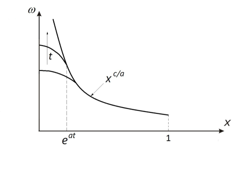
Figure 1: Illustration to Eq.-s (23),(24): dependence of vorticity distribution on time.

What happens if there is another boundary condition? Substituting arbitrary boundary condition $\omega(t,1)=f(t)$ and $t^{\prime}(t,x):x=e^{a(t-t^{\prime})}$, we have

$$\omega(t,x)=x^{c/a}f\left(t-\frac{1}{a}\ln x\right)\rightarrow_{t\to\infty}x^{c/a}f(t)$$

for any given $x$. Thus, any reasonable (i.e., slower than exponential) function $f$ does not change the power law and affects only the coefficient, which becomes time-dependent (see Fig.2). Since the boundary conditions correspond to large scales, the characteristic time for $f(t)$ is of the order of the largest eddy turnover time. This statement is also valid for the general case (17).

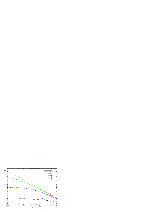
Figure 2: Evolution of vorticity distribution in one particular case: $a=-3,b=1$, $\omega_{0}(x)=1/\left(1+\left[x+0.1\sin(10\pi x)\right]^{2/3}\right)$, $\omega(t,1)=1/\left(e^{-2t}+\left[1+0.1e^{-3t}\sin(10\pi e^{3t})\right]^{2/3}\right)$. One can see that the range of strong oscillations drifts to smaller $x$, while inside the ’inertial range’ the fluctuations become negligible and the power law dominates.

IV.1 Evolution of spectrum

The solution (23),(24) is not stationary: there is always a narrowing non-stationary region $x<\bar{x}(t)$. We now consider this solution in terms of Fourier transform. This is useful to understand the spectrum evolution (which gives the basis to the idea of cascade), and to take account of viscosity. The Fourier transform of vorticity is:⁷

$$\omega(t,k)=e^{ct}\int\limits_{0}^{\bar{x}(t)}e^{ikx}\omega_{0}(xe^{-at})dx+\int\limits_{\bar{x}(t)}^{\infty}e^{ikx}x^{c/a}dx$$

The first integral can be rewritten as

$$e^{ct}e^{at}\int_{0}^{1}e^{ikye^{at}}\omega_{0}(y)dy\simeq e^{-bt}\omega_{0}(ke^{at})$$

It depends weakly on $k$ for all $k<\bar{k}=e^{-at}$, and decreases exponentially as a function of time. The second integral is

$$k^{b/a}\int\limits_{k\bar{x}(t)}^{\infty}e^{iy}y^{c/a}dy$$

It is a power law for $k<e^{-at}$ and decreases sharply at larger $k$.

So, $\omega(t,k)$ is a step function of $k$, with the step running exponentially to the right as time goes.

To illustrate this, we consider one particular solution of (19), for which the Fourier transform is easy to count analytically. This time we do not demand the ’strong’ boundary condition (21); as we have found in previous subsection, it is enough for $\omega(t,1)$ not to grow exponentially. Let initial distribution of vorticity be

$$\omega_{0}(x)=\left(1+ix\right)^{c/a}+\left(1-ix\right)^{c/a}$$

In accordance with (19),(22) evolution of $\omega(t,x)$ takes the form:

$$\omega(x,t)=e^{ct}\left[\left(1+ie^{-at}x\right)^{c/a}+\left(1-ie^{-at}x\right)^{c/a}\right]$$

$$=2e^{ct}\left(1+x^{2}e^{-2at}\right)^{c/2a}cos\,(\phi c/a)$$

where $\tan\,\phi=xe^{-at}$. For $x\gg e^{at}$, we have $\phi\simeq\pi/2$, $\omega\propto x^{c/a}$.

The Fourier transform of this function is:

$$\omega(k,t)=|k|^{b/a}e^{-|k|e^{at}}$$ (25)

The spectrum falls exponentially at $k\sim\bar{x}^{-1}=e^{-at}$. The result is similar to the effect of viscosity, but the cutoff moves along the $k$ axis towards larger values of $k$ (in case of dissipation the cutoff would not depend on time).

Such a step spectrum spreading to larger $k$ is usually interpreted as a cascade, or breaking of vortices. We see that in our approach it appears without a cascade, and energy is transported to smaller scales by means of the narrowing transition region near one selected point, which is to become a singular point at infinite time.

It is usually assumed that viscosity is necessary to get stationary statistical picture in turbulence. Indeed, one needs viscosity to make all statistical averages, e.g., structure functions of all orders, stationary: energy injected into a flow at large scales has to be dissipated at viscous scale.

However, our example shows that, in some cases, stationary spatial probabilistic distribution can be reached even without dissipation in some finite range of scales.

IV.2 Effect of viscosity

It is easy to generalize (18) to include viscosity. Since $\nabla u$ is directed along $x$ axis, the equation takes the form:

$$\frac{\partial u(x,t)}{\partial t}+ax\frac{\partial u(x,t)}{\partial x}+bu(x,t)=\nu\frac{\partial^{2}u}{\partial x^{2}}$$

Similarly, the viscous term should be added into the right-hand side of (19). Changing to the new variable $q=xe^{-at}$, we get

$$\frac{\partial\omega(q,t)}{\partial t}-c\omega(q,t)=\nu e^{-2at}\frac{\partial^{2}\omega}{\partial q^{2}}$$

(We recall that $a<0$.) The Fourier transformation gives:

$$\omega(k,t)=e^{-bt}\omega_{0}(ke^{at})e^{\frac{\nu}{2a}k^{2}(1-e^{2at})}$$

It appears that, while non-stationarity produces a ’step’ (exponential fall) running to the right with exponential speed $k\sim e^{-at}$, viscosity produces a similar (but sharper) step which runs to the left, and very quickly (after $t\sim 1/2|a|$) becomes stationary at $k\sim\sqrt{2|a|/\nu}$.

For the particular example of initial condition considered in the previous subsection, instead of (25) we then get

$$\omega(k,t)=|k|^{b/a}e^{-|k|e^{at}}e^{\frac{\nu}{2a}k^{2}(1-e^{2at})}$$

We see that the ’non-viscous’ solution does not differ from the ’viscous’ solution in the range $k<e^{-at}$, $k<\sqrt{2|a|/\nu}$.

Although the non-viscous equation does not ’smoothen’ the initial perturbations, it transports them to smaller and smaller scales and multiplies by a decreasing term. So, the solutions of Euler and Navier-Stokes equations behave similarly in the limit $t\to\infty$, $\nu\to 0$. In this sense, the Euler equation can be treated as the inviscid NSE.

V Introduction of stochastics

In the previous section, the large-scale velocity fluctuations are treated as deterministic ones. We have seen that this causes a power-law dependence of vorticity. This would provide a scaling dependence of velocity structure functions, but it would be mono-fractal, instead of multifractal: the scaling exponents would be proportional to their numbers. The multifractal picture can be restored if we take stochastic behavior of large-scale fluctuations into account.

The Theorems cited in page 4 claim that the ’systematic’ part (12) of randomly changing matrix (10) not only has exponentially growing averages, but also fluctuations of these exponents are Gaussian random processes. An accurate analysis of the stochastic equation (6) with account of these fluctuations could probably allow to construct a complete theory. In this paper, however, we restrict ourselves by the simplified example from the previous Section.

According to the Theorems, the stochastic generalization of (19) has the form:

$$\frac{\partial\omega}{\partial t}+(a+\xi_{1}(t))x\frac{\partial\omega}{\partial x}-(c+\xi_{2}(t))\omega=0$$ (26)

Here $\xi_{1}(t)$ and $\xi_{2}(t)$ are Gaussian random processes with zero averages.

All the relations of the previous Section can be rewritten for this case; e.g., (22) becomes

$$\omega(t,x)=e^{c(t-t^{\prime})+\int\limits_{t^{\prime}}^{t}\xi_{2}(t^{\prime\prime})dt^{\prime\prime}}\omega\left(t^{\prime},xe^{-a(t-t^{\prime})-\int\limits_{t^{\prime}}^{t}\xi_{1}(t^{\prime\prime})dt^{\prime\prime}}\right)$$

For $x=0$, taking $t^{\prime}=0$, we get

$$\omega(t,0)=e^{ct+\int\limits_{0}^{t}\xi_{2}(t^{\prime\prime})dt^{\prime\prime}}\omega(0,0)$$

Let $\xi_{1},\xi_{2}$ be delta-correlated with dispersions $D_{1}$ and $D_{2}$. (For more general case of not delta-correlated processes see Appendix 1.) The probability density can then be written as

$$dP[\xi_{1}(t),\xi_{2}(t)]=e^{-\frac{\int\xi_{1}(t^{\prime})^{2}dt^{\prime}}{2D_{1}}}e^{-\frac{\int\xi_{2}(t^{\prime})^{2}dt^{\prime}}{2D_{2}}}\prod\limits_{t}d\xi_{1}(t)d\xi_{2}(t)$$

Thus,

$$\left<\omega(t,0)^{n}\right> = e^{nct}\langle e^{n\int\limits_{0}^{t}\xi_{2}dt}\rangle\omega^{n}(0,0)$$ (27)

$$= e^{nct}\int e^{\int\limits_{0}^{t}\left(-\frac{\xi_{2}^{2}}{2D_{2}}+n\xi_{2}\right)dt}d\xi_{2}(t)\omega^{n}(0,0)$$

$$= e^{nct+n^{2}D_{2}t/2}\omega^{n}(0,0)$$

We see that the averages diverge exponentially as a function of time. This characterizes the solution inside the non-stationary inner region (24) with growing vorticity. The width $\bar{x}$ of the non-stationary region is determined by the condition

$$\bar{x}e^{-at-\int\xi_{1}dt}\simeq 1$$

But, since $\int\xi_{1}dt\propto\sqrt{t}$ after long time, we have $at\gg\int\xi_{1}dt$ and $\bar{x}\simeq e^{at}$.

Thus, adding stochastic fluctuations to $a$ and $c$ increases the central growth of vorticity but does not change significantly the size of the non-stationary region.

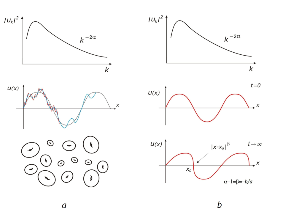
Figure 3: Cascade model (a) vs Infinite-time singularity (b): the same spectrum is produced by different physical processes

To understand the statistical properties, however, we are interested in the outer region $x>\bar{x}(t)$. In this case, by analogy with (23), we choose $t^{\prime}(x,t)$ in such a way that

$$\ln x=a(t-t^{\prime})+\int\limits_{t^{\prime}}^{t}\xi_{1}dt^{\prime\prime}$$ (28)

Then

$$\omega(t,x)=e^{c(t-t^{\prime})+\int\limits_{t^{\prime}}^{t}\xi_{2}dt^{\prime\prime}}\omega(t^{\prime},1)$$ (29)

The value $t^{\prime}(x,t)$ is now a random process. An accurate calculation of averages of (29) is very complicated, so we just make an estimate. We restrict ourselves by small $x$, so $\left|\ln x\right|\gg 1$. An average of $\int\xi_{1}dt^{\prime\prime}$ is zero, so we can estimate it by $\int\xi_{1}dt^{\prime\prime}\propto\sqrt{t-t^{\prime}}$. Thus, in (28) this term is much smaller than $a(t-t^{\prime})$ and can be neglected. From (29) we then have

$$\omega(t,x)\simeq x^{c/a}e^{\int\limits_{t-t^{\prime}}^{t}\xi_{2}dt^{\prime\prime}}\omega(t^{\prime},1)$$

Raising to the power $n$ and taking an average, we get

$$\langle\omega^{n}\rangle = x^{nc/a}\int e^{\int\left(-\frac{\xi_{2}^{2}}{2D_{2}}+n\xi_{2}\right)dt^{\prime\prime}}\prod\limits_{t}d\xi_{2}(t)\omega^{n}(t^{\prime},1)$$ (30)

$$\propto x^{n\frac{c}{a}}e^{n^{2}\frac{D_{2}}{2}(t-t^{\prime})}\propto x^{n\frac{c}{a}+n^{2}\frac{D_{2}}{2a}}$$

This scaling of vorticity moments is equivalent to velocity structure functions with nonlinear scaling exponents:

$$\langle\Delta v^{n}(l)\rangle\sim\langle\omega^{n}\rangle l^{n}\sim l^{\zeta_{n}}\ ,\quad\zeta_{n}=-\frac{b}{a}n+\frac{D_{2}}{2a}n^{2}$$ (31)

The obtained relations provide an explanation of the nonlinear dependence of scaling exponents on their order.

The exponential average growth of vorticity in the vicinity of local maxima and power-law distribution near these points (23), (24) produce the linear term in (31), while the fluctuations (29) are responsible for the non-linearity.

VI Discussion

In this paper we derive existence and properties of vortex filaments (high-vorticity regions) on the basis of the stochastic Eq.(6) (which in turn is derived from the NSE) by using the Theorems (page 4). The main result is the scaling behavior of vorticity (17),(23) inside these vortex filaments, without suggesting finite-time singularities, and multifractal behavior of vorticity (30) and velocity (31) statistical moments. Thus, in our approach the direct, not only probabilistic formulation of the Multifractal model is valid, however there are no singularities in the flow: at any finite time peaks of vorticity are smoothed inside constantly narrowing non-stationary regions.

In the ’canonical’ cascade interpretation of the power-law spectrum, vortices of all scales are presented and contribute to the resulting scaling (Fig. 3a). To the opposite, our consideration shows that the same spectrum is produced by small regions near some ’almost singular’ points (Fig. 3b). Excluding these regions would cut the spectrum up to $k\sim l^{-1}$, and the scales are easy to separate. An evidence for this second approach comes from the numerical simulations Farge : the observed ’coherent structures’ with high vorticity, i.e. vortex filaments, are found to be very stable, the lifetime exceeding many times the largest-eddy turnover time. This contradicts to the idea of cascade. In Farge it is shown that these small-scale structures are responsible for the 5/3 law. Picking them out breaks the power-law energy spectrum in the whole inertial range.

The assumptions and simplifications used throughout the work are rather general and do not seem crucial. We restricted our consideration by symmetric large-scale velocity gradients $A_{ij}$, supposing that the large-scale vorticity can be neglected inside the vortex filament: the solution can probably be generalized for all $A_{ij}$.

Even the simplified ’straightened’ model, apart from its illustrative functions, can be valid in the high-vorticity regions: the rotation matrix $s$ in (11), being a large-scale value, has a characteristic time of changes $\tau_{cor}\gg\omega^{-1}$, and hence its rotation can be treated as an adiabatic process.

Unfortunately, the numerical values of the coefficients $\lambda_{i}$ (and hence the coefficients in (30), (31)) are not defined by the Theorems. They depend on the properties of the random large-scale fluctuations, and a special investigation is needed to derive them. However, one can consider some restrictions and particular cases. In Falkovich , for a similar case of polar decomposition (for which similar theorems are valid), the coefficient analogous to $\lambda_{2}$ is shown to be zero if the probability distribution $A_{ij}$ is Gaussian. The same is true for the Iwasawa decomposition considered in our paper; moreover, $\lambda_{2}$ is zero for all large-scale configurations that are statistically isotropic:

$$P(A)=P(RAR^{-1})$$

for any rotation $R$, and satisfy the condition

$$P[A_{ij}(t)]=P[-A_{ij}(t)]$$ (32)

(see Appendix 2). This requirement is stronger than the single condition of isotropy: for example, let matrix $A_{ij}$ take the values $A=R\cdot\mbox{diag}(\alpha,\beta,\gamma)\cdot R^{-1}$, where $\alpha,\beta,\gamma$ are some definite (not random) quantities and $R$ is a random orthogonal matrix, $R\in SO(3)$. The process is isotropic if $P(A)$ does not depend on $R$. However, $P(A)\neq P(-A)$, since the value $-A$ is impossible.

More generally, if the distribution of traceless symmetric random matrix $A_{ij}$ is isotropic, its probability density may depend on only two parameters, e.g., $P(A)=P(\mbox{tr}A^{2},\mbox{tr}A^{3})$. The additional condition $P(A)=P(-A)$ means that $P$ is an even function of its the second argument.

The value $A_{ij}$ is defined in (5) as $\partial U_{i}/\partial r_{j}$ where $\bf U$ is a velocity. Hence, the transformation $A\to-A$ is time reversal, and the condition (32) is time conjugation invariance.

Thus, T-invariance leads to $\lambda_{2}=0$; it also implies even dependence of probability density on $\mbox{tr}A^{3}$, in particular, $\langle\mbox{tr}A^{3}\rangle=0$. On the other hand, the large-scale process that produces turbulence must provide some flux of energy from outside into the flow. This breaks the T-symmetry: indeed, the contribution of the large-scale velocity component (5) to the average energy flux through any sphere of intermediate radius $\bar{r}\ll L$ is

$$\langle\Phi\rangle=\langle\int U^{2}{\bf U}d{\bf s}\rangle=\langle A_{ij}A_{im}A_{kp}\int\bar{r}_{j}\bar{r}_{m}\bar{r}_{k}\frac{\bar{r}_{p}}{\bar{r}}\bar{r}^{2}d\Omega\rangle$$

$$=\langle 2\mbox{tr}A^{3}4\pi\frac{\bar{r}^{5}}{3\cdot 3}\rangle\propto\langle\mbox{tr}A^{3}\rangle$$

The condition $\langle\Phi\rangle<0$ then gives $\langle\mbox{tr}A^{3}\rangle<0$, (for the ’straightened’ model this means $b=-\lambda_{2}>0$, compare to the signs of $a,b,c$ in (20)).

So, symmetry $t\to-t$ is forbidden if we require the income of energy into the flow. Thus, $\lambda_{2}$ must not be zero, and $P(A)\neq P(-A)$. This means, in particular, that Gaussian probability density is not valid for $P(A)$. (This does not contradict to the experiments that show Gaussian behavior of large-scale velocity, since (5) is valid for scales $l\ll L$ only.)

However, we recall that, independently on the statistics of the large-scale fluctuations, the Theorems state that fluctuations of the exponents (12) are Gaussian.

Returning to the higher-order structure functions, the relation (31) proves their power-law dependence and provides an explanation of the nonlinear dependence of scaling exponents on their order. As it was shown in PRE2 ; notPRE , the quadratic nonlinearity describes very well velocity scaling exponents observed in experiments and numerical simulations. More accurate analysis of the stochastic equations, with account of rare events which are of most importance for high-order structure functions, would of course add higher degrees to the expression. But even this simplified consideration appears to be enough to show that average large-scale exponents $\lambda_{i}$ in (12) determine the scaling (’fractal’) behavior of the solutions, while fluctuations of these exponents produce ’multifractality’.

VII Conclusion

Thus, in the paper we study the solutions of the Navier-Stokes equation in the regions of high vorticity (vortex filaments), treating the large-scale velocity fluctuations as independent stationary random process. The stochastic equations (4), (6) are thus the main equations of the paper.

We analyze the long-time asymptote of the solutions to Eq. (6) and show that an infinite-time singularity appears in the limit $\nu\to 0,l\to 0$; for any finite $t$, there is no singularity, and for any finite $l$ inside the inertial range, the solution becomes a power law (17) after some time $t(l)$.

We show that the solution corresponds to random rotation and systematic exponential stretching of a vortex filament. This exponential stretching causes the power-law distribution of vorticity, the resulting spectrum is quite similar to that expected from the model of breaking vortices.

Taking into account the stochastic component of the stretching, we derive the multi-scaling distribution of vorticity (and velocity differences), and quadratic dependence of velocity scaling exponents on their order (31). As it was shown in PRE2 , this result agrees very well with experimental and DNS data. All these results do not depend on the assumptions on the properties of the large-scale random process.

We are grateful to Prof. A.V. Gurevich for his permanent interest to our work. We thank Prof. V.S. L’vov and A.S. Ilyin for valuable discussion and the first anonymous referee for useful comments and questions.

The work was partially supported by RAS Program 18 $\Pi$.

VIII Appendix 1: Calculation of statistical moments in the case of finite time-correlated random process

The averages (27), (30) are calculated under the assumption of delta-correlated coefficients $\xi_{1},\xi_{2}$ in Eq. (26). However, the same result can be obtained in the limit $t\to\infty$ without the assumption. To illustrate this, we consider the average $\langle e^{k\int\limits_{0}^{t}a(t_{1})dt_{1}}\rangle$ where $a(t)$ is a random Gaussian process with correlation function

$$\langle a(t_{1})a(t_{2})\rangle=G(t_{1}-t_{2})\ ,\quad\int\limits_{-\infty}^{\infty}d\tau G(\tau)=1$$ (33)

The probability density of $a$ can be written in the form SlavnovFaddeev :

$$P[a](t)=e^{-\frac{1}{2}\int\limits_{0}^{t}dt_{1}\int\limits_{0}^{t}dt_{2}G^{-1}(t_{1}-t_{2})a(t_{1})a(t_{2})}$$

where $G^{-1}$ is defined by

$$\int_{-\infty}^{\infty}dt^{\prime}G(t_{2}-t^{\prime})G^{-1}(t^{\prime}-t_{1})=\delta(t_{2}-t_{1})$$ (34)

For the statistical moments we then get

$$\langle e^{k\int\limits_{0}^{t}a(t_{1})dt_{1}}\rangle=$$

$$=\int\prod\limits_{\tau}da(\tau)e^{-\frac{1}{2}\int\limits_{0}^{t}dt_{1}\int\limits_{0}^{t}dt_{2}G^{-1}(t_{1}-t_{2})a(t_{1})a(t_{2})+k\int\limits_{0}^{t}dt_{1}a(t_{1})}$$

This is a Gaussian integral, thus, the saddle-point method gives an exact result in the case SlavnovFaddeev . The optimal trajectory is defined by the condition:

$$\left.\frac{\delta}{\delta a(\tau)}\right|_{a(\tau)=a_{0}(\tau)}\left(-\frac{1}{2}\int\limits_{0}^{t}dt_{1}\int\limits_{0}^{t}dt_{2}G^{-1}(t_{1}-t_{2})a(t_{1})a(t_{2})\right.$$

$$\left.+k\int\limits_{0}^{t}dt_{1}a(t_{1})\right)=0$$

Hence,

$$\int\limits_{0}^{t}dt_{1}G^{-1}(t^{\prime}-t_{1})a_{0}(t_{1})=k\ ,\quad 0<t^{\prime}<t$$ (36)

Making use of (34), we get

$$a_{0}(t^{\prime})=k\int\limits_{0}^{t}dt_{1}G(t^{\prime}-t_{1})$$ (37)

Substituting to (VIII) we get

$$\langle e^{k\int\limits_{0}^{t}a(t_{1})dt_{1}}\rangle \simeq \exp\left[\int\limits_{0}^{t}a_{0}(t_{1})dt_{1}\times\right.$$

$$\times \left.\left(-\frac{1}{2}\int\limits_{0}^{t}dt_{2}G^{-1}(t_{1}-t_{2})a_{0}(t_{2})+k\right)\right]$$

and with account of (36), (37):

$$\langle e^{k\int\limits_{0}^{t}a(t_{1})dt_{1}}\rangle \simeq \exp\left[\frac{1}{2}k\int\limits_{0}^{t}dt_{1}a_{0}(t_{1})\right]$$

$$= \exp\left[\frac{1}{2}k^{2}\int\limits_{0}^{t}dt_{1}\int\limits_{0}^{t}dt_{2}G(t_{1}-t_{2})\right]$$

(One could as well obtain the same result by shifting $a(t)$ to get the perfect square in the exponent.)

From (VIII) it follows that as $t\to\infty$ (or, more precisely, for any $t$ larger than the correlation time) the statistical moments grow exponentially, just as in the case of delta-correlated process.

IX Appendix 2: On the coefficients $\lambda_{i}$ in the case of isotropic large-scale random process $A_{ij}(t)$.

We consider a random isotropic traceless symmetric matrix $A_{ij}(t)$. Denote $\gamma=qq^{T}$, where the matrix $q$ is defined by (8). The matrix $\gamma$ is thus a functional of the random process $A_{ij}(t)$.

From (10), with account of $A=A^{T}$, we have:

$$\gamma(-A)\gamma(A)=q(-A)q^{T}(-A)q(A)q^{T}(A)=I$$

Hence, $\gamma^{-1}(A)=\gamma(-A)$. According to the Iwasawa decomposition, $\gamma=zd^{2}z^{T}$; in particular,

$$(d^{2})_{33}=\gamma_{33}\ ,$$

$$(d^{2})_{11}=(\gamma_{22}\gamma_{33}-\gamma_{23}^{2})^{-1}=\left((\gamma^{-1})_{11}\right)^{-1}=\left(\gamma(-A)_{11}\right)^{-1}$$

(We recall that and $\mbox{det}\gamma=\mbox{det}q(A)=1$.)

For any analytic function $f(B)$ and any rotation $R\in SO(3)$, $f(RBR^{-1})=Rf(B)R^{-1}$. Taking $f=\gamma$,  $B=-A$, and $R=R_{c}=\left(\begin{array}[]{ccc}0&0&-1\\ 0&1&0\\ 1&0&0\end{array}\right)$, we get $\gamma(-A)=R_{c}^{-1}\gamma(-R_{c}AR_{c}^{-1})R_{c}$, so

$$\left(\gamma(-A)\right)_{11}=\gamma(-R_{c}AR_{c}^{-1})_{33}$$

Now, from Theorem 1 (page 4) we have

$$\lambda_{3} = \lim\limits_{N\to\infty}\langle\frac{1}{2N}\log(d^{2})_{33}\rangle$$ (39)

$$= \lim\limits_{N\to\infty}\frac{1}{2N}\int\log\left(\gamma(A)\right)_{33}P(A)DA(t)$$

$$\lambda_{1} = \lim\limits_{N\to\infty}\langle\frac{1}{2N}\log(d^{2})_{11}\rangle$$

$$= - \lim\limits_{N\to\infty}\frac{1}{2N}\int\log\left[\gamma(-R_{c}AR_{c}^{-1})_{33}\right]P(A)DA(t)$$

We recall that the integral means $\int\prod\limits_{t}\prod\limits_{i,j}dA_{ij}(t)P[A(t)]$. The last expression can be rewritten as

$$\lambda_{1}=-\lim\limits_{N\to\infty}\frac{1}{2N}\int\log\left[\gamma(A^{\prime})_{33}\right]P(-R_{c}^{-1}A^{\prime}R_{c})DA^{\prime}(t)$$

Isotropy of the distribution means $P(A)=P(A^{\prime})$, $A^{\prime}=RAR^{-1}$ for any $R\in SO(3)$. Taking $R=R_{c}$, we get

$$\lambda_{1}=-\lim\limits_{N\to\infty}\frac{1}{2N}\int\log\left[\gamma(A^{\prime})_{33}\right]P(-A^{\prime})DA^{\prime}(t)$$

Comparison with (39) shows that if $P(A)=P(-A)$, then $\lambda_{1}=-\lambda_{3}$ (and, since $\mbox{tr}A=0$, $\lambda_{2}=0$). This condition corresponds to a symmetry produced by the transformation $A\to-A$. Recalling the definition of $A$ (5) one can see that this symmetry corresponds to the time reverse.

If time reversal invariance does not hold, we have no general relations for the values of $\lambda_{i}$.

References

- (1) F.Toschi and E.Bodenschatz Annu. Rev. Fluid Mech. 41: 375, 2009.
- (2) R.Benzi, L.Biferale, R.Fisher et al J.Fluid. Mech. 653: 221, 2010.
- (3) A.Arneodo, R. Benzi, J. Berg et al.,Phys. Rev. Lett. 100, 254504 (2008)
- (4) G. Parisi, U. Frisch in: Turbulence and Predictability in Geophysical Fluid Dynamics, Proceed. Intern. School of Physics ’E.Fermi’, 1983, Varenna, Italy; North-Holland, Amsterdam edited by. M. Ghil, R. Benzi, and G. Parisi 84-87, 1985.
- (5) G. Boffetta, A. Mazzino and A. Vulpiani Journal of Physics A 41, 363001 (2008).
- (6) U. Frisch, ’Turbulence. The legacy of A.N. Kolmogorov’, Cambridge Univ. Press, Cambridge, 1995
- (7) E.A. Kuznetsov, V.P.Ruban, JETP, 91, 775-785 (2000)
- (8) P. Orlandi, S. Pirozzoli and G. F. Carnevale, J. Fluid Mech., 690, 288-320 (2012).
- (9) C.M. Meneveau, K.R. Sreenivasan J. Fluid Mech. 224, 429 (1991)
- (10) B. Mandelbrot Proc. Royal Soc. London A 434, 79 (1991)
- (11) Z.S.She, E.Jackson, S.A.Orszag Proc.R.Soc.Lond.A 434,101 (1991)
- (12) N. Okamoto, K. Yoshimatsu, K. Schneider et al Phys.Fluids 19, 115109 (2007)
- (13) K.P. Zybin, V.A. Sirota, A.S. Ilyin, Physica D: Nonlinear Phenomena 241, 269 (2012)
- (14) K.P. Zybin, V.A. Sirota, Phys.Rev.E 85, 056317, 2012
- (15) K.P. Zybin, V.A. Sirota arXiv:1204.1465 [physics.flu-dyn]
- (16) V A Sirota and K P Zybin Phys. Scr. T155 014005 (2013)
- (17) Ya.B. Zel’dovich, A.A. Ruzmaikin, S.A. Molchanov and D.D. Sokoloff J. Fluid Mech bf 144, 1 (1984)
- (18) G. Falkovich, K. Gawedzki, M. Vergassola Rev. Mod. Phys. 73(4) 913-975 (2001)
- (19) N.V. Antonov, M. Hnatich, J. Honkonen, M. Jurcisin, Phys. Rev. E 68, 046306 (2003)
- (20) A.V. Letchikov Russian Math. Surveys, 51 (1), 49 96 (1996)
- (21) H. Furstenberg, Trans.Amer. Math. Soc. 108, 377-428 (1963)
- (22) V.N. Tutubalin Theory Probab. Appl. 10(1) 15-27 (1965)
- (23) V.N. Tutubalin Theory Probab. Appl. 22(2) 203-214 (1977)
- (24) V.N. Tutubalin Theory Probab. Appl. 14(2) 313-319 (1969)
- (25) V.N. Tutubalin Theory Probab. Appl., 13(1) 65-83 (1968)
- (26) A.A. Slavnov, L.D. Faddeev Gauge Fields: An Introduction to Quantum Theory; WESTVIEW Press (1994)