POWER FACTOR FOR LAYERED
THERMOELECTRIC MATERIALS WITH A CLOSED
FERMI SURFACE IN A QUANTIZING MAGNETIC FIELD

Abstract

The field dependence of the power factor for a layered thermoelectric material with a closed Fermi surface in a quantizing magnetic field and at helium temperatures has been studied in the geometry where the temperature gradient and the magnetic field are perpendicular to the material layers. The calculations are carried out in the constant relaxation time approximation. In weak magnetic fields, the layered-structure effects are shown to manifest themselves in a phase retardation of power factor oscillations, increase of their relative contribution, and certain reduction of the power factor in whole. In high magnetic fields, there exists an optimal range, where the power factor reaches its maximum, with the corresponding value calculated for the chosen parameters of the problem in the effective mass approximation being by 12% higher than that for real layered crystals. Despite low temperatures, the power factor maximum obtained with those parameters in a magnetic field of 1 T has a value characteristic of cuprate thermoelectric materials at 1000 K. For this phenomenon to take place, it is necessary that the ratio between the free path of charge carriers and the interlayer distance should be equal to or larger than 30,000. However, in ultraquantum magnetic fields, the power factor drastically decreases following the dependence $P\propto T^{-3}B^{-6}$. The main reason for this reduction is a squeeze of the Fermi surface along the magnetic field in the ultraquantum limit owing to the condensation of charge carriers on the bottom of a single filled Landau subband.

1 Introduction

Nowadays, the thermoelectric properties of many materials are intensively studied. The objects of researches are metals, alloys, semiconductors [1,​ 2], fullerenes [3], composites [4], including biomorphic ones [5], etc. A promising thermoelectric material is graphene [6]. The specific photothermoelectric effect in graphene, which was considered earlier as of exclusively the photovoltaic origin, allows it to be considered as a material for solar cells with a high efficiency.

The theory of thermoelectric properties for various substances, including nanosystems [7,​ 8], is intensively developed. For instance, one of the first works devoted to the theory of transverse thermoelectric coefficients of metals in a quantizing magnetic field has been published by A.M. Kosevich and V.V. Andreev [9].

A large number of substances under investigation – e.g., the semiconductor A^IIIB^VIC^VII systems, intercalated compounds of graphite, synthetic metals on the basis of organic compounds, graphene, and others belong to the layered materials according to their crystal structure. At the same time, in the overwhelming majority of theoretical works dealing with the behavior of such layered systems in quantizing magnetic fields, only the transverse galvano-magnetic effects are studied as a rule. The thermal conductivity of graphene in a magnetic field, including the quantizing one, its electric dc and ac conductivities, and the quantum Hall effect were considered in works [10,​ 11]. In those works, the Fermi surface (FS) of graphene was assumed to be open, i.e., it occupies the whole one-dimensional Brillouin zone and is connected, if being periodically continued; in other words, it looks like a continuous corrugated cylinder. The cited works were mainly devoted to the research of the charge carrier behavior in a layer plane. Therefore, the concept of “massless neutrino” with the linear dependence of the energy on the quasimomentum in the layer plane turned out to be an effective tool for the description of the band structure in graphene. In this case, the energy levels in a quantizing magnetic field were determined in the framework of the effective Hamiltonian method.

On the other hand, in the previous works, the author showed that, if the behavior of charge carriers in the direction perpendicular to the layers is studied, the layered-structure effects can be well pronounced in the case of a closed FS as well [12] or if the topological transition from the open FS to a closed one takes place [13].

It should be noticed that the power factor, which equals the product of the squared thermoelectric coefficient and the conductivity, is rather an indicative integrated characteristic for the system of free charge carriers in a material [14]. This is of importance for the estimation of thermoelectric properties of and applications. Therefore, this work was aimed at calculating and researching the dependence of the power factor for a layered thermoelectric material with a closed FS on the induction of a quantizing magnetic field.

2 Calculation of the Power Factor for a Layered Crystal and Discussion of the Results Obtained

While calculating the power factor for a layered crystal in a quantizing magnetic field directed perpendicularly to the layer planes, the following dispersion law for the charge carriers will be used:

$$\varepsilon\left({n,x}\right)=\mu^{\ast}B\left({2n+1}\right)+W\left(x\right)\!,$$ (1)

where $\mu^{\ast}=\mu_{\rm B}{m_{0}}/m^{\ast}$, $\mu_{\rm B}$ is the Bohr magneton, ${m_{0}}$ the free electron mass, $m^{\ast}$ the effective electron mass in a layer plane, $B$ the magnetic field induction, $n$ the Landau level number, $W\left(x\right)$ the dispersion law for charge carriers along the superlattice axis, $x=ak_{z}$, $k_{z}$ is the component of the quasimomentum along the superlattice axis, and $a$ the distance between translationally equivalent layers.

In order to study the influence of layered-structure effects on the power factor, the latter will be calculated in two cases. These are the strong coupling approximation,

$$W\left(x\right)=\Delta\left({1-\cos x}\right)\!,$$ (2)

where $\Delta$ is the miniband halfwidth that governs the motion of electrons between the layers, and the case where only the term quadratic in $x$ is retained in the series expansion of formula (2), which corresponds to the effective mass approximation. In both cases, the dependence of chemical potential in the electron gas on the magnetic field induction is taken into account. To simplify calculations, the relaxation time for charge carriers will be considered constant. With the same purpose in view, the influence of Dingle factor on longitudinal conductivity oscillations (Shubnikov–de Haas oscillations) and oscillations of the longitudinal thermoelectric coefficient $\alpha_{zz}$ (the latter is defined, to within the sign accuracy, as the proportionality coefficient between the electrochemical potential gradient in the system of charge carriers and the temperature gradient, provided that the current equals zero). It should be noticed, however, that the indicated factor can play a substantial role at the electron scattering by impurities and defects in the crystal lattice [15].

If we proceed from the Boltzmann kinetic equation and act in the same way as when deriving the formula for the longitudinal electroconductivity, the following general formula for the thermoelectric coefficient $\alpha_{zz}$ can be obtained:

$$\alpha_{zz}=-\left[{\frac{\partial}{\partial T}\sum\limits_{\gamma}{\tau_{\gamma}g_{\gamma}v_{z\gamma}^{2}f^{0}\left({\varepsilon_{\gamma}}\right)}}\right]\times$$

$$\times\left[{e\frac{\partial}{\partial\zeta}\sum\limits_{\gamma}{\tau_{\gamma}g_{\gamma}v_{z\gamma}^{2}f^{0}\left({\varepsilon_{\gamma}}\right)}}\right]^{-1}\!.$$ (3)

Here, $T$ is the absolute temperature, $e$ the elementary charge, $\zeta$ the chemical potential of the system of charge carriers (we consider them to be electrons), $\gamma\equiv\left({n,x}\right)$ a set of quantum numbers that characterize the electron energy, $\tau_{\gamma}$ the relaxation time for charge carriers, $v_{z\gamma}$ the longitudinal electron velocity, $g_{\gamma}$ the statistical weight of a Landau level per unit volume of the crystal, and $f^{0}\left({\varepsilon_{\gamma}}\right)$ the Fermi–Dirac distribution function. For the dispersion law (1) and provided that $\tau_{\gamma}\equiv\tau\left(x\right)$, formula (3) becomes

$$\alpha_{zz}=\frac{\pi k}{e}\frac{A}{B+C}.$$ (4)

The quantities $A$, $B$, and $C$ are

$$A\!=\!\sum\limits_{l=1}^{\infty}\left({-1}\right)^{l-1}f_{l}^{\rm th}\!\!\!\!\!\!\!\int\limits_{W\left(x\right)\leq\zeta}\!\!\!\!\!\!\!\tau\left(x\right){W}^{\prime}\left(x\right)^{2}\times$$

$$\times\sin\left[{\pi l\frac{\zeta-W\left(x\right)}{\mu^{\ast}B}}\right]dx,$$ (5)

$$B=0.5\int\limits_{W\left(x\right)\leq\zeta}{\tau\left(x\right){W}^{\prime}\left(x\right)^{2}dx},$$ (6)

$$C\!=\!\sum\limits_{l=1}^{\infty}\left({-1}\right)^{l}f_{l}^{\sigma}\!\!\!\!\!\!\int\limits_{W\left(x\right)\leq\zeta}\!\!\!\!\!\!\tau\left(x\right){W}^{\prime}\left(x\right)^{2}\times$$

$$\times\cos\left[{\pi l\frac{\zeta-W\left(x\right)}{\mu^{\ast}B}}\right]dx,$$ (7)

where

$$f_{l}^{\rm th}=\left[{{\mathrm{sh}}\left({{\pi^{2}lkT}\mathord{\left/{\vphantom{{\pi^{2}lkT}{\mu^{\ast}B}}}\right.\kern-1.2pt}{\mu^{\ast}B}}\right)}\right]^{-1}\times$$

$$\times\left[{1-\left({{\pi^{2}lkT}\mathord{\left/{\vphantom{{\pi^{2}lkT}{\mu^{\ast}B}}}\right.\kern-1.2pt}{\mu^{\ast}B}}\right){\mathrm{cth}}\left({{\pi^{2}lkT}\mathord{\left/{\vphantom{{\pi^{2}lkT}{\mu^{\ast}B}}}\right.\kern-1.2pt}{\mu^{\ast}B}}\right)}\right]\!,$$ (8)

$$f_{l}^{\sigma}=\left({{\pi^{2}lkT}\mathord{\left/{\vphantom{{\pi^{2}lkT}{\mu^{\ast}B}}}\right.\kern-1.2pt}{\mu^{\ast}B}}\right)\left[{{\mathrm{sh}}\left({{\pi^{2}lkT}\mathord{\left/{\vphantom{{\pi^{2}lkT}{\mu^{\ast}B}}}\right.\kern-1.2pt}{\mu^{\ast}B}}\right)}\right]^{-1}\!.$$ (9)

In accordance with the results of work [12], the total longitudinal electric conductivity of a layered crystal can be written down in the form

$$\sigma_{zz}=\frac{32\pi^{2}e^{2}m^{\ast}a}{h^{4}}\left({B+C}\right)\!.$$ (10)

Hence, the power factor equals

$$P=\frac{32\pi^{4}k^{2}m^{\ast}aA^{2}}{h^{4}\left({B+C}\right)}.$$ (11)

In the case of the dispersion law (2) and $\tau\left(x\right)\equiv\tau_{0}$, it is easy to pass to the dimensionless coefficients $A$, $B$, and $C$ and write down the power factor as

$$P=\frac{16\pi^{4}k^{2}m^{\ast}a\Delta^{2}\tau_{0}A^{2}}{h^{4}\left({B+C}\right)}.$$ (12)

Now, the coefficients $A$, $B$, and $C$ are as follows:

$$A=\sum\limits_{l=1}^{\infty}({-1})^{l-1}f_{l}^{\mathrm{th}}\biggl{\{}\!\sin\left(\!{\pi l\frac{\zeta-\Delta}{\mu^{\ast}B}}\!\right)\!\biggl{[}\!\left({C_{0}-C_{2}}\right)\times$$

$$\times J_{0}\left(\!\frac{\pi l\Delta}{\mu^{\ast}B}\!\right)+\sum\limits_{r=1}^{\infty}{\left({-1}\right)^{r}\left(2C_{2r}-C_{2r+2}-C_{2r-2}\right)}\times$$

$$\times J_{2r}\left(\!\frac{\pi l\Delta}{\mu^{\ast}B}\!\right)\!\biggr{]}+\cos\left(\!\pi l\frac{\zeta-\Delta}{\mu^{\ast}B}\!\right)\sum\limits_{r=0}^{\infty}{\left({-1}\right)^{r}}\times$$

$$\times\left(2C_{2r+1}-C_{2r+3}-C_{\left|{2r-1}\right|}\right)J_{2r+1}\left(\!\frac{\pi l\Delta}{\mu^{\ast}B}\!\right)\!\biggr{\}}\!,$$ (13)

$$B=0.5\left({C_{0}-C_{2}}\right)\!.$$ (14)

$$C=\sum\limits_{l=1}^{\infty}\left({-1}\right)^{l}f_{l}^{\sigma}\biggl{\{}\cos\left(\!\pi l\frac{\zeta-\Delta}{\mu^{\ast}B}\!\right)\!\biggl{[}\left({C_{0}-C_{2}}\right)\times$$

$$\times J_{0}\left(\!{\frac{\pi l\Delta}{\mu^{\ast}B}}\!\right)+\sum\limits_{r=1}^{\infty}{\left({-1}\right)^{r}\left({2C_{2r}-C_{2r+2}-C_{2r-2}}\right)}\times$$

$$\times J_{2r}\left(\!\frac{\pi l\Delta}{\mu^{\ast}B}\!\right)\!\biggr{]}-\sin\left(\!\pi l\frac{\zeta-\Delta}{\mu^{\ast}B}\!\right)\sum\limits_{r=0}^{\infty}\left({-1}\right)^{r}\times$$

$$\times(2C_{2r+1}-C_{2r+3}-C_{\left|{2r-1}\right|})J_{2r+1}\left(\!{\frac{\pi l\Delta}{\mu^{\ast}B}}\!\right)\!\biggr{\}}\!.$$ (15)

In formulas (13)–(15), $J_{n}\left(x\right)$ are the Bessel functions of the first kind of a real argument. The modulating coefficients $C_{m}$ are defined as follows:

$$C_{0}=\arccos\left(\!{1-\frac{\zeta-\mu^{\ast}B}{\Delta}}\!\right)\!,$$ (16)

$$C_{m}=\frac{\sin mC_{0}}{m}form\neq 0.$$ (17)

In the approximation concerned, formulas (12)–(17) completely determine the temperature and field dependences of the power factor for a layered crystal, with the chemical potential of a gas of charge carriers in formulas (16) and (17) being considered to depend on the magnetic field. Owing to the FS squeezing in a crystal in the quantizing magnetic field, the quantity $\mu^{\ast}B$, i.e. the minimum electron energy, is subtracted from the chemical potential.

In the effective mass approximation, the dimensionless coefficients $A$, $B$, and $C$ look like

$$A=\sum\limits_{l=1}^{\infty}(-1)^{l-1}f_{l}^{\rm th}\Biggl{\{}\frac{\mu^{\ast}B}{\pi l\Delta}\sqrt{\frac{2\left({\zeta-\mu^{\ast}B}\right)}{\Delta}}-$$

$$-\frac{1}{\pi}\left(\!\frac{\mu^{\ast}B}{l\Delta}\!\right)^{\!3/2}\Biggl{[}\cos\left(\!{\frac{\pi l\zeta}{\mu^{\ast}B}}\!\right)C\left(\!\sqrt{2l\left(\!{\frac{\zeta}{\mu^{\ast}B}-1}\!\right)}\!\right)+$$

$$+\sin\left(\!{\frac{\pi l\zeta}{\mu^{\ast}B}}\!\right)S\left(\!{\sqrt{2l\left(\!{\frac{\zeta}{\mu^{\ast}B}-1}\!\right)}}\!\right)\!\Biggr{]}\!\Biggr{\}}\!,$$ (18)

$$B=\frac{1}{6}\left[\!{2\left(\!{\frac{\zeta-\mu^{\ast}B}{\Delta}}\!\right)\!}\right]^{\!3\mathord{\left/{\vphantom{32}}\right.\kern-1.2pt}2}\!,$$ (19)

$$C=\sum\limits_{l=1}^{\infty}(-1)^{l}f_{l}^{\sigma}\frac{1}{\pi}\left(\!\frac{\mu^{\ast}B}{l\Delta}\!\right)^{\!3/2}\!\Biggl{[}\sin\left(\!{\frac{\pi l\zeta}{\mu^{\ast}B}}\!\right)\times$$

$$\times C\left(\!\sqrt{2l\left(\!\frac{\zeta}{\mu^{\ast}B}-1\!\right)}\!\right)-\cos\left(\!\frac{\pi l\zeta}{\mu^{\ast}B}\!\right)\times$$

$$\times S\left(\!\sqrt{2l\left(\!\frac{\zeta}{\mu^{\ast}B}-1\!\right)}\!\right)\!\Biggr{]}\!.$$ (20)

Here, $C\left(x\right)$ and $S\left(x\right)$ are the Fresnel cosine and sine integrals, respectively.

For further calculations, the dependence of chemical potential for the gas of charge carriers on the quantizing magnetic field is required. In work [12], this dependence was already presented, but it is useful to recall it. The equation that determines the chemical potential of the electron gas in a quantizing magnetic field at low temperatures has the following general form:

$$n_{0}=\frac{4m^{\ast}}{ah^{2}}\!\!\int\limits_{W\left(x\right)\leq\zeta}\!\!\!\!{\left[{\zeta-W\left(x\right)}\right]dx}+\frac{8\pi m^{\ast}kT}{ah^{2}}\times$$

$$\times\sum\limits_{l=1}^{\infty}{\frac{\left({-1}\right)^{l}}{{\mathrm{sh}}\left({{\pi^{2}lkT}\mathord{\left/{\vphantom{{\pi^{2}lkT}{\mu^{\ast}B}}}\right.\kern-1.2pt}{\mu^{\ast}B}}\right)}}\!\!\int\limits_{W\left(x\right)\leq\zeta}\!\!\!\!{\sin\left(\!{\pi l\frac{\zeta-W\left(x\right)}{\mu^{\ast}B}}\!\right)dx},$$ (21)

where $n_{0}$ is the bulk concentration of charge carriers in the crystal. For the dispersion law (2) and in the case of a closed FS, Eq. (21) reads

$$n_{0}=\frac{4m^{\ast}\Delta}{ah^{2}}\left[{\left({\gamma-1}\right)C_{0}+\sqrt{2\gamma-\gamma^{2}}}\right]+$$

$$+\frac{8m^{\ast}\pi kT}{ah^{2}}\sum\limits_{l=1}^{\infty}{\frac{\left({-1}\right)^{l}}{{\mathrm{sh}}\left({{\pi^{2}lkT}\mathord{\left/{\vphantom{{\pi^{2}lkT}{\mu^{\ast}B}}}\right.\kern-1.2pt}{\mu^{\ast}B}}\right)}}\Bigg{\{}\!{\sin\left(\!{\pi l\frac{\zeta-\Delta}{\mu^{\ast}B}}\!\right)\times}$$

$$\times\left[{C_{0}J_{0}\left(\!{\frac{\pi l\Delta}{\mu^{\ast}B}}\!\right)+2\sum\limits_{r=1}^{\infty}{\left({-1}\right)^{r}C_{2r}}J_{2r}\left(\!{\frac{\pi l\Delta}{\mu^{\ast}B}}\!\right)}\!\right]+$$

$${+{2\cos}\left(\!{\pi l\frac{\zeta-\Delta}{\mu^{\ast}B}}\!\right)\sum\limits_{r=0}^{\infty}{\left({-1}\right)^{r}C_{2r+1}J_{2r+1}\left(\!{\frac{\pi l\Delta}{\mu^{\ast}B}}\!\right)}}\!\Bigg{\}}\!.$$ (22)

The modulating coefficients $C_{m}$ in this equation should be taken at $B=0$, with $\gamma=\zeta/\Delta$ at that.

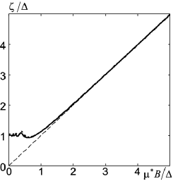
Fig. 1.: Field dependence of the chemical potential at $\gamma_{0}=$ $=1$ and ${kT/\Delta=0.03}$ for a layered crystal (solid curve) and in the effective mass approximation (dashed curve). Thin dashed line corresponds to the limiting case $\zeta=\mu^{\ast}B$

In the case of an open FS, i.e. at $\gamma-{\mu^{\ast}B}/\Delta\geq 2$, we have to put $C_{0}=\pi$ in formulas (13)–(17) and (22), and, in addition, consider the radical in formula (22) equal to zero.

In the effective mass approximation, Eq. (22) takes the form

$$n_{0}=\frac{8m^{\ast}\zeta}{3ah^{2}}\sqrt{\frac{2\zeta}{\Delta}}+\frac{8\pi m^{\ast}kT}{ah^{2}}\sqrt{\frac{\mu^{\ast}B}{\Delta}}\times$$

$$\times\sum\limits_{l=1}^{\infty}{\frac{\left({-1}\right)^{l}}{l^{1\mathord{\left/{\vphantom{12}}\right.\kern-1.2pt}2}{\rm sh}\left(\!{{\pi^{2}lkT}\mathord{\left/{\vphantom{{\pi^{2}lkT}{\mu^{\ast}B}}}\right.\kern-1.2pt}{\mu^{\ast}B}}\right)}}\left[{\sin\left(\!{\frac{\pi l\zeta}{\mu^{\ast}B}}\!\right)C\left(\!{\sqrt{\frac{2l\zeta}{\mu^{\ast}B}}}\!\right)}\right.\!\!+$$

$$\left.{+\cos\left(\!{\frac{\pi l\zeta}{\mu^{\ast}B}}\leavevmode\nobreak\ \right)S\left(\!{\sqrt{\frac{2l\zeta}{\mu^{\ast}B}}}\!\right)}\!\right]\!.$$ (23)

The concentrations of charge carriers in both examined cases will be considered identical and determined by the formula

$$n_{0}=\frac{4m^{\ast}\Delta}{ah^{2}}\!\left[\!{\left({\gamma_{0}\!-\!1}\right)\arccos\left({1\!-\!\gamma_{0}}\right)\!+\!\sqrt{2\gamma_{0}\!\!-\gamma_{0}^{2}}}\right]\!\!,\!$$ (24)

where $\gamma_{0}={\zeta_{0}}/\Delta$, and ${\zeta_{0}}$ is the Fermi energy of the crystal electron gas with the dispersion law (2) at the zero temperature and in the absence of a magnetic field.

The solutions of Eqs. (22) and (23) can be found numerically, The corresponding results obtained for the layered crystal with a closed FS is presented in Fig. 1 in the range $0<\mu^{\ast}B/\Delta<5$. If the magnetic field grows, both curves approach each other, because Eq. (22) has the following asymptotic solution in strong quantizing magnetic fields in the case of a closed FS [12]:

$$\zeta\left(B\right)=\mu^{\ast}B+\Delta\left[{1-\cos\left(\!{\frac{f\left({\gamma_{0}}\right)\Delta}{2\mu^{\ast}B}}\!\right)\!}\right]\!.$$ (25)

In the case of a closed FS,

$$f\left({\gamma_{0}}\right)=\left({\gamma_{0}-1}\right)\arccos\left({1-\gamma_{0}}\right)+\sqrt{2\gamma_{0}-\gamma_{0}^{2}},$$ (26)

whence one can see that the single filled Landau subband gets narrower in the ultraquantum limit, and this narrowing has to be taken into account while calculating the power factor.

In the effective mass approximation, formula (25) acquires the form

$$\zeta\left(B\right)=\mu^{\ast}B+\frac{\Delta^{3}f^{2}\left({\gamma_{0}}\right)}{8\left({\mu^{\ast}B}\right)^{2}}.$$ (27)

Note that all the formulas presented above for the longitudinal thermoelectric coefficient and the power factor were obtained under the condition that the interaction-induced broadening of energy levels is small in comparison with the distance between Landau levels. Only in this case, the broadening of energy levels can be directly connected with the relaxation time, and the shift of energy levels associated with the scattering can be neglected. Then, the approach based on the Boltzmann equation is completely equivalent to that based on the Kubo formalism.

For the calculation of the power factor, we also need an expression for the relaxation time $\tau_{0}$. For any $\gamma_{0}$, this quantity can be determined in the same way as in works [12,​ 13], namely, by the formula

$$\tau_{0}=\frac{lm_{es}^{\ast}}{hk_{0}}.$$ (28)

Here, $l$ is the mean free path of charge carriers, which is determined by the scattering at impurities; $k_{0}$ the radius of an equivalent sphere, by which the real FS is substituted for the scattering to be considered as isotropic; and $m_{es}^{\ast}$ the equivalent mass of charge carriers at this sphere. The two latter parameters are so defined that the concentration of charge carriers and the Fermi energy coincide with the corresponding parameters determined either for the real layered crystal or in the effective mass approximation. Therefore, in both cases,

$$k_{0}=\sqrt[3]{\frac{12\pi^{2}m^{\ast}\Delta f\left({\gamma_{0}}\right)}{ah^{2}}}.$$ (29)

At the same time, for a real layered crystal, the parameter $m_{es}^{\ast}$ is determined by the formula

$$m_{es}^{\ast}=\frac{h^{2}k_{0}^{2}}{8\pi^{2}\gamma_{0}\Delta},$$ (30)

and, in the effective mass approximation, by the formula

$$m_{es}^{\ast}=\frac{h^{2}k_{0}^{2}}{8\pi^{2}\gamma_{0em}\Delta}.$$ (31)

Therefore, we obtain the following ultimate expression for the power factor of the crystal:

$$P=P_{0}\frac{A^{2}}{B+C},$$ (32)

where the parameter $P_{0}$ is determined by the formula

$$P_{0}=\frac{2\pi^{3}k^{2}m^{\ast}a^{2}\Delta}{h^{3}\gamma_{0}}\sqrt[3]{\frac{12\pi^{2}m^{\ast}\Delta f\left({\gamma_{0}}\right)}{ah^{2}}}N$$ (33)

for a real layered crystal and by the formula

$$P_{0}=\frac{2\pi^{3}k^{2}m^{\ast}a^{2}\Delta}{h^{3}\gamma_{0em}}\sqrt[3]{\frac{12\pi^{2}m^{\ast}\Delta f\left({\gamma_{0}}\right)}{ah^{2}}}N$$ (34)

in the effective mass approximation. The coefficients $A$, $B$, and $C$ in formula (32) are determined by formulas (13)–(15) for the real layered crystal and by formulas (18)–(20) in the effective mass approximation. In addition, $N\equiv l/a$.

The calculation results for the field dependence of the power factor obtained for a layered crystal in various ranges of the quantizing magnetic field induction are depicted in Figs. 2 and 3. From Fig. 2, one can see that, in the case of a real layered crystal, the oscillations of the power factor are more pronounced, but the corresponding absolute values are smaller in comparison with those in the effective mass approximation. Similarly to the case of longitudinal conductivity, this fact can be explained, because, on the one hand, any confinement imposed on the free motion of charge carriers reduces the conductivity and, on the other hand, the dependence of the cross-section area of the FS by the plane perpendicular to the magnetic field direction on the longitudinal quasimomentum is weaker. Moreover, in the case of a real layered crystal, a certain phase delay of oscillations takes place. This happens, because the Fermi energy for a real layered crystal is slightly lower than that in the effective mass approximation, provided the same concentration of charge carriers. The same factor is also responsible for the increase of the relative contribution of oscillations to the power factor.

In the conventional quasiclassical approximation, the power factor equals

$$P=P_{0}\frac{3\left({\mu^{\ast}B}\right)^{3}}{2^{3/2}\pi^{2}\Delta^{3/2}\zeta^{3/2}}\times$$

$$\times\left[{\sum\limits_{l=1}^{\infty}{\left({-1}\right)^{l-1}l^{-3/2}f_{l}^{\rm th}\cos\left(\!{\frac{\pi l\zeta}{\mu^{\ast}B}-\frac{\pi}{4}}\!\right)}}\!\right]^{2}\!.$$ (35)

This formula also makes it evident that, if the Fermi energy is constant, it is impossible to distinguish the influence of layered-structure effects on the power factor. However, since the Fermi energy for a real layered crystal is slightly lower than that in the effective mass approximation at a constant concentration of charge carriers, the power factor oscillations have to be more pronounced in the former case, which really takes place. At the same time, Fig. 2 testifies that the power factor is a little larger in the effective mass approximation than that in the case of real layered crystal, although formula (35), with regard for formulas (33) and (34), brings about the opposite conclusion. Such an apparent contradiction arises because the value of power factor is also affected by the monotonous component of the thermoelectric coefficient, which cannot be taken into account in the framework of the traditional approach, for which the specific shape and the size of a FS are insignificant.

From Fig. 3, one can see that, in strong quantizing magnetic fields, the power factor oscillations are also more pronounced in the case of real layered crystal than those in the effective mass approximation. However, after having passed the last oscillation minimum, the power factor starts to grow considerably and reaches a maximum approximately at the point of the last oscillation peak for the chemical potential. The presence of this maximum can be explained by the following physical reasoning. On the one hand, it is clear that, in accordance with the general thermodynamic relations – with which formula (35), as well as formulas (13) and (18) and Figs. 2 and 3, are in full agreement – the power factor has tend to zero at weak enough magnetic fields and low enough temperatures. On the other hand, it should also tend to zero in the ultraquantum limit as a result of the FS squeezing along the magnetic field direction. However, this factor cannot be equal to zero identically. Hence, it has to possess a maximum at a certain induction of the magnetic field. In addition, the figure demonstrates that the power factor maximum is larger and more pronounced in the effective mass approximation than that in the case of real layered crystal. It is explained by a higher electron density of states and its more drastic dependence on the energy for a real layered crystal. However, for the same reason, the power factor after passing the maximum falls down more slowly in the case of real layered crystal than that in the effective mass approximation.

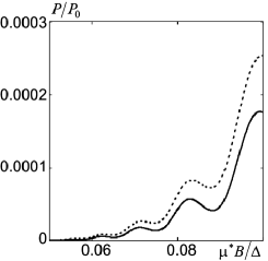
Fig. 2.: Field dependences of the power factor at $\gamma_{0}=1$ and $kT/\Delta=0.03$ calculated for a real layered crystal (solid curve) and in the effective mass approximation (dotted curve) in the interval $0.05\leq{\mu^{\ast}B}/\Delta\leq 0.1$

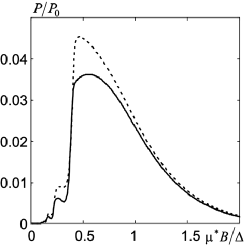
Fig. 3.: The same as in Fig. 2, but in the interval $0\leq{\mu^{\ast}B}/\Delta\leq 2$

The results of numerical calculations show that, for instance, at $\Delta=0.01\leavevmode\nobreak\ \mathrm{eV}$, $m^{\ast}=0.01m_{0}$, $kT/\Delta=$ $=0.03$, $a=1\mathrm{\leavevmode\nobreak\ nm}$, and $\gamma_{0}=1$, the power factor in the maximum equals $3.350\times 10^{-9}N\leavevmode\nobreak\ \mathrm{W}/(\mathrm{m\cdot K}^{2})$ for a real layered crystal and $3.758\times 10^{-9}N\leavevmode\nobreak\ \mathrm{W}/(\mathrm{m\cdot K}^{2})$ in the effective mass approximation. On the other hand, promising are those thermoelectric materials, for which the power factor equals, e.g., $1.04\times$ $\times 10^{-4}\leavevmode\nobreak\ \mathrm{W}/(\mathrm{m\cdot K}^{2})$ – to tell the truth, this value was obtained at 1000$\leavevmode\nobreak\ \mathrm{K}$ [14]. Under our conditions, such a value of power factor corresponds to $N=({2.767\div 3.104})\times 10^{4}$, i.e. the mean free path of charge carriers is $l={28\div 31}$ $\mu\mathrm{m}$. For such a ratio between the mean free path and the distance between the neighbor layers, putting the Dingle factor identically equal to 1 within the whole range of examined magnetic fields is completely eligible. Those data can be regarded as a specific variant of “technological requirements” to the thermoelectric material. Provided the same parameters, the magnetic field induction, at which the power factor reaches its maximum, amounts to approximately 1.018 T.

At last, let us derive the asymptotic law for the power factor recession in the ultraquantum limit. For this purpose, expression (27) should be substituted for $\zeta$ in expressions (5)–(7) for the coefficients $A$, $B$, and $C$. As a result, $\left({-1}\right)^{l}$ becomes compensated owing to the trigonometric multipliers. Then, the cosines and the sines are put equal to 1 and to their arguments, respectively. The expression $f_{l}^{th}$ at ${\mu^{\ast}B/kT\gg 1}$ looks like

$$f_{l}^{\mathrm{th}}=\frac{\left({{\pi^{2}lkT}\mathord{\left/{\vphantom{{\pi^{2}lkT}{\mu^{\ast}B}}}\right.\kern-1.2pt}{\mu^{\ast}B}}\right)^{2}}{2{\mathrm{sh}}\left({{\pi^{2}lkT}\mathord{\left/{\vphantom{{\pi^{2}lkT}{\mu^{\ast}B}}}\right.\kern-1.2pt}{\mu^{\ast}B}}\right)}.$$ (36)

While summing up the series over $l$, let us take into account that the numerical analysis testifies to the validity of the following relations at small $\delta$:

$$\sum\limits_{l=1}^{\infty}{\frac{\delta l}{\sinh\left({\delta l}\right)}=\frac{2.467}{\delta}},$$ (37)

$$\sum\limits_{l=1}^{\infty}{\frac{\delta l^{3}}{\sinh\left({\delta l}\right)}=\frac{12.176}{\delta^{3}}}.$$ (38)

The integrands in formulas (5)–(7) are expanded in series in $x$ to an accuracy of the leading terms and integrated within the limits from 0 to $\frac{f\left({\gamma_{0}}\right)\Delta}{2\mu^{\ast}B}$. After carrying out all transformations and combining numerical multipliers, the following asymptotic expression is obtained for the power factor of a real layered crystal near the ultraquantum limit:

$$P=1.929\times 10^{-2}k^{2}f^{7}\left({\gamma_{0}}\right)\frac{m^{\ast}a^{2}\Delta^{10}}{h^{3}\left({\mu^{\ast}B}\right)^{6}\left({kT}\right)^{3}\gamma_{0}}\times$$

$$\times\sqrt[3]{\frac{m^{\ast}\Delta f\left({\gamma_{0}}\right)}{ah^{2}}}N.$$ (39)

In the effective mass approximation, the power factor of the crystal equals

$$P=1.929\times 10^{-2}k^{2}f^{7}\left({\gamma_{0}}\right)\frac{m^{\ast}a^{2}\Delta^{10}}{h^{3}\left({\mu^{\ast}B}\right)^{6}\left({kT}\right)^{3}\gamma_{0em}}\times$$

$$\times\sqrt[3]{\frac{m^{\ast}\Delta f\left({\gamma_{0}}\right)}{ah^{2}}}N.$$ (40)

Hence, for the parameters given above and at $B=$ $=60\leavevmode\nobreak\ \mathrm{T}$, we obtain $P=3.780\times 10^{-11}\leavevmode\nobreak\ \mathrm{W}/(\mathrm{m\cdot K}^{2})$ for a real layered crystal and $P=3.635\times$$\times 10^{-11}\leavevmode\nobreak\ \mathrm{W}/(\mathrm{m\cdot K}^{2})$ in the effective mass approximation. Thus, the power factor decreases by six orders of magnitude in comparison with its maximum value. Therefore, although the asymptotic law $P\propto B^{-6}T^{-3}$ is a little hard to understand, because the power factor does not vanish at $T=0$, which contradicts, at first sight, the general thermodynamic principles, this law does not lead to incorrect physical consequences at real low temperatures.

It should be noted that if the same approach as that used in the calculation of the longitudinal conductivity in works [12,​ 16] be applied while calculating the power factor at low temperatures near the ultraquantum limit, the thermoelectric coefficient, as well as the power factor, would be identically equal to zero, because the sum under the sign of derivative in the numerator of formula (3) does not depend on the temperature in the framework of this approach. Therefore, this approach all the same demands that the thermoelectric coefficient should be calculated in the next approximation in the small parameters ${kT}/\zeta_{0}$, ${kT}/\Delta$, and ${kT}/{\mu^{\ast}B}$. However, it is not a subject of this paper.

3 Conclusions

Hence, it is demonstrated that the layered-structure effects at closed Fermi surfaces and in weak quantizing magnetic fields can manifest themselves as a phase delay of oscillations of the power factor, an increase of the relative contribution of oscillations to the power factor magnitude, and a simultaneous reduction of the latter. However, in stronger magnetic fields, namely, at the point where the chemical potential of the system of charge carriers has the last oscillation maximum, the power factor reaches its maximum value. The layered-structure effects in strong magnetic fields near the ultraquantum limit reveal themselves as more pronounced oscillations of the power factor, a reduction of the maximum value, a smearing of the peak in the dependence of the power factor on the magnetic field, and a slower recession of the power factor after passing through the maximum.

In weak quantizing magnetic fields, the power factor tends to zero obeying the law $P\propto B^{3}$. In strong magnetic fields, near the ultraquantum limit, it vanishes following the law $P\propto T^{-3}B^{-6}$. At the same time, the amplitude of the power factor maximum in perfect enough specimens with the ratio $l/a\geq 30000$ can be comparable with the corresponding values for the best cuprate-based thermoelectric materials at 1000$\leavevmode\nobreak\ \mathrm{K}$.

It is clear that all the results of this paper need an experimental verification. However, to the author’s knowledge, all relevant experiments concern galvano-magnetic effects in layered crystals with a strongly open FS in the interval where the quasiclassical approximation is applicable. One of a few exceptions is an old work [17] dealing with the Shubnikov–de Haas effect in graphite intercalated with bromine, where just the topological transition was considered from the open to the closed FS at the growth of the bromine concentration.

It is rather difficult for the author to judge about direct practical applications of the results of his theoretical researches. Nevertheless, he hopes that this research will stimulate the statement of new experiments to study thermoelectric and thermomagnetic phenomena in layered crystals, including those with a closed FS. The latter circumstance, in the author’s opinion, can be important for the development of novel thermoelectric materials.

П.В. Горський
ФАКТОР ПОТУЖНОСТI
ШАРУВАТОГО ТЕРМОЕЛЕКТРИЧНОГО
МАТЕРIАЛУ IЗ ЗАМКНЕНОЮ ПОВЕРХНЕЮ
ФЕРМI В КВАНТУЮЧОМУ МАГНIТНОМУ ПОЛI
Р е з ю м е
Дослiджено залежнiсть фактора потужностi шаруватого термоелектричного матерiалу iз замкненою поверхнею Фермi в квантуючому магнiтному полi при гелiєвих температурах для випадку, коли магнiтне поле та градiєнт температури спрямованi перпендикулярно до шарiв. Розрахунки проведено в наближеннi сталого часу релаксацiї. У слабких магнiтних полях ефекти шаруватостi виражаються у вiдставаннi осциляцiй фактора потужностi за фазою, збiльшеннi їх вiдносного внеску i у деякому зменшеннi величини фактора потужностi в цiлому. В областi сильних магнiтних полiв iснує оптимальний дiапазон, в якому фактор потужностi рiзко зростає i досягає максимуму, абсолютна величина котрого при вибраних параметрах задачi в наближеннi ефективної маси на 12% бiльша, нiж для реального шаруватого кристала. Попри низькi температури, при цих параметрах максимум фактора потужностi в магнiтному полi з iндукцiєю близько 1 Тл досягає значення, характерного для перспективних купратних термоелектричних матерiалiв при температурi понад 1000 К. Для цього необхiдно, щоб вiдношення довжини вiльного пробiгу носiїв заряду до вiдстанi мiж сусiднiми шарами становило 30000 або бiльше. Однак в ультраквантових магнiтних полях фактор потужностi рiзко знижується за законом $P\propto T^{-3}B^{-6}$. Основною причиною такого зниження є стиск поверхнi Фермi в напрямку магнiтного поля в ультраквантовiй границi внаслiдок конденсацiї носiїв заряду на днi єдиної заповненої пiдзони Ландау з номером $n=0$.

References

- [1] M.M. Gadzhialiev and Z.Sh. Pirmagomedov, Fiz. Tekh. Poluprovodn. 43, 1032 (2009).
- [2] F.F. Aliev, Fiz. Tekh. Poluprovodn. 37, 1082 (2003).
- [3] V.A. Kul’bachinskii, V.G. Kytin, V.D. Blank, S.G. Buga, and M.Yu. Popov, Fiz. Tekh. Poluprovodn. 45, 1241 (2011).
- [4] L.N. Lukyanova, V.A. Kutasov, V.V. Popov, and P.P. Konstantinov, Fiz. Tverd. Tela 46, 1366 (2004).
- [5] A.I. Shelyh, B.I. Smirnov, T.S. Orlova, I.A. Smirnov, A.R. de Arellano-Lopez, J. Martinez-Fernandes, and F.M. Varela-Feria, Fiz. Tverd. Tela 48, 214 (2006).
- [6] N.M. Gabor, J.C.W. Song, Q. Ma, N.L. Nair, T. Taychatanapat, K. Watanabe, T. Taniguchi, L.S. Levitov, and P. Jarilo-Herrero, Science 334, 648 (2011).
- [7] D.A. Pshenaj-Severin and M.I. Fedorov, Fiz. Tverd. Tela 49, 1559 (2007).
- [8] Y.S. Liu, X.K. Hong, J.F. Feng, and X.F. Yang, Nanoscale Res. Lett. 6, 618 (2011).
- [9] A.M. Kosevich and V.V.Andreev. Zh. Eksp. Teor. Fiz. 38, 882 (1960).
- [10] V.P. Gusynin and S.G. Shaparov. Phys. Rev. B 71, 125124 (2005).
- [11] M. Müller, L. Frits, and S. Sachdev. arXiv: 0805.1413v2 (2008).
- [12] P.V. Gorskyi, Ukr. Fiz. Zh. 55, 1297 (2010).
- [13] P.V. Gorskyi, Fiz. Tekh. Poluprovodn. 45, 928 (2011).
- [14] V.L. Matukhin, I.Kh. Khabibullin, D.A. Shulgin, S.V. Shmidt, and E.I. Terukov, Fiz. Tekh. Poluprovodn. 46, 1126 (2012).
- [15] D. Shoenberg, Magnetic Oscillations in Metals (Cambridge Univ. Press, Cambridge, 1984).
- [16] B. Laikhtman and D. Menashe, Phys. Rev. B 52, 8974 (1994).
-
[17]
A.S. Bender and D.A. Young, Phys. Status. Solidi B
47, K95 (1974).
Received 03.06.12.
Translated from Ukrainian by O.I. Voitenko
П.В.
Горський