Cooperative Synchronization in Wireless Networks

Abstract

Synchronization is a key functionality in wireless network, enabling a wide variety of services. We consider a Bayesian inference framework whereby network nodes can achieve phase and skew synchronization in a fully distributed way. In particular, under the assumption of Gaussian measurement noise, we derive two message passing methods (belief propagation and mean field), analyze their convergence behavior, and perform a qualitative and quantitative comparison with a number of competing algorithms. We also show that both methods can be applied in networks with and without master nodes. Our performance results are complemented by, and compared with, the relevant Bayesian Cramér–Rao bounds.

I Introduction

Wireless networks (WNs) must deliver a wide variety of services, assuming a decentralized, but cooperative operation of the WN. Many of these services have stringent requirements on time alignment among the nodes in the WN, while each node has its individual local clock. Usually these clocks are counters driven by a local oscillator, and differences appear in counter offsets and in oscillator frequencies. Time alignment is necessary, e.g., for cooperative transmission and distributed beamforming [1], time-division-multiple-access communication protocols [2], duty-cycling [3], and localization and tracking methods [4, 5], or location based control schemes [6]. In these tasks, the representation of specific time instants requires low clock offsets, while for accurate representation of time intervals, strict frequency alignment is necessary. To guarantee correct operation, the clocks need to be aligned up to a certain application-specific accuracy.

Synchronization is a widely studied topic. Existing network synchronization schemes differ mainly in how local time information is encoded, exchanged, and processed [7]. In this work, we will limit ourselves to so-called packet-coupled synchronization, whereby local time is encoded in time stamps and exchanged via packet transmissions [8]. Commonly used algorithms, which consider both offset and frequency synchronization, are the Reference Broadcast Synchronization (RBS) [9] and the Flooding Time Synchronization Protocol (FTSP) [10]. Both methods require a specified network structure and do not perform synchronization in a distributed manner. This increases communication and computation overhead to maintain the structure, makes the network more vulnerable to node failures, and reduces the scalability. More recent synchronization algorithms work fully distributed, and are well suited to cooperative networks. For offset and frequency estimation, there are methods based on consensus [11, 12, 13, 14], and gradient descent [15]. They typically suffer from slow convergence speed, and thus require the exchange of a high number of data packets in the network to achieve a desired accuracy. Recently, distributed Bayesian estimators were proposed, which provide a maximum a posteriori (MAP) estimate using belief propagation (BP) on factor graphs (FG). The successful application of offset synchronization in [16, 17] showed superior estimation accuracy and higher convergence rate than competing distributed algorithms, in the case when a master node (MN) with reference time is available. The extension to joint offset and frequency synchronization is not straightforward, as nonlinear dependencies are introduced in the measurement model and thus in the likelihood of the measurements. In parallel to this work, [18] proposed such an extension by modifying the measurement equations. This modification restricts measurement model and results in an auxiliary function rather than a likelihood function. Thus, no MAP solution is obtained. A general drawback of BP in [16, 18] is the high computational complexity, scaling quadratically in the number of neighbors.

In this paper, we build on the work from [16], considering both relative clock phases (offsets) and clock frequencies (skews). Our contributions are as follows:

• Based on a measurement model from experimental data, we derive an approximate, yet accurate statistical model that allows a Gaussian reformulation of the MAP estimation of the clock parameters.

• We propose a BP and a mean field (MF) message passing algorithm based on the statistical model. When MNs are available, MF provides highly accurate synchronization with low computational complexity. To the best of our knowledge, this is the first application of MF to the network synchronization problem.

• We provide convergence conditions for BP and MF synchronization with and without MNs.

• We derive a Bayesian Cramér–Rao bound (BCRB), which serves as a fundamental performance bound for the case when prior information on the local clock parameters is available.

The remainder of this paper is organized as follows: In Section II, we introduce the clock model, the network model, and the measurement protocol. In Section III, we provide an overview of the state-of-the-art on distributed synchronization, under both phase and skew uncertainties. Exact and simplified statistical models of measurement likelihoods and clock priors are derived in Section IV, followed by a description of the BCRB in Section V. The simplified models from Section IV are used to derive two Bayesian algorithms based on message passing in Section VI. In Section VII, we numerically study the properties of the proposed algorithms and compare them to state-of-the-art algorithms from Section III. Finally, we draw our conclusions in Section VIII.

II System Model

II-A Network Model

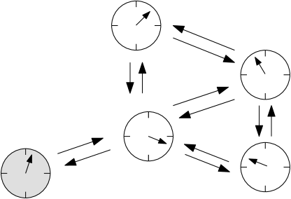
Figure 1: Connectivity graph of a wireless network with $M=1$ MN (shaded) and $A=4$ agent nodes.

We consider a static network comprising a set $\mathcal{M}\triangleq\{1,\ldots,M\}$ of MNs and a set $\mathcal{A}\triangleq\{M+1,\ldots,N\}$ of agent nodes (ANs) (see Fig. 1). The $M=|\mathcal{M}|$ fully synchronous MNs impose a common time reference to the network. The $A=|\mathcal{A}|$ ANs have imperfect clocks that may not run synchronously with the reference time.

The topology is defined by the communication set $\mathcal{C}\subseteq\mathcal{I}\!\times\mathcal{I}$. If two nodes $i,j\in\mathcal{I}$ can communicate, then $(i,j)\!\in\!\mathcal{C}$ and $(j,i)\!\in\!\mathcal{C}$. Connections among MNs are not considered, i.e., $(i,j)\notin\mathcal{C}$ if $i,j\!\in\!\mathcal{M}$. For each $i\!\in\!\mathcal{A}$ we define a neighborhood set $\mathcal{T}_{i}\subseteq\mathcal{I}\setminus\!\{i\}$ that includes all $j\!\in\!\mathcal{I}$ that communicate with $i$, i.e., $j\!\in\!\mathcal{T}_{i}$ if and only if $(i,j)\!\in\!\mathcal{C}$.

The network is assumed to be connected, so that there is a path between every pair of nodes.

II-B Clock Model

Each network node $i$ possesses a clock displaying local time $c_{i}(t)$, related to the reference time $t$ by

$$c_{i}(t)=\alpha_{i}t+\beta_{i},$$ (1)

where $\beta_{i}$ is the clock phase of node $i$ and $\alpha_{i}$ is the clock skew of node $i$ [8]. When $i\in\mathcal{M}$, $\alpha_{i}\!=\!1$ and $\beta_{i}\!=\!0$. When $i\in\mathcal{A}$, both $\alpha_{i}$ and $\beta_{i}$ are considered as random variables. The clock phase $\beta_{i}$ depends on the initial network state, and can be modeled with an uninformative prior (e.g., as uniformly distributed over a large range, or, equivalently, having Gaussian distribution with a large variance $\sigma_{\beta,i}^{2}$ [16]). The clock skew $\alpha_{i}$ depends on the quality of the clocks, typically expressed in parts per million (ppm), and is modeled as a Gaussian random variable [20] with mean 1 and variance $\sigma_{\alpha,i}^{2}$. Nodes with more sophisticated clocks will have smaller $\sigma_{\alpha,i}^{2}$. Note that in reality the clock skews $\alpha_{i}$ are not static over time, as they change with ambient environment variations (e.g., temperature). Such variations are typically much slower than the update rate of synchronization protocols, and can thus safely be ignored.

The following notation will be convenient: $\bm{\theta}_{i}=[\alpha_{i},\beta_{i}]^{\mathrm{T}}$, $\bm{\vartheta}_{i}=[\lambda_{i},\nu_{i}]^{\mathrm{T}}=[1/\alpha_{i},\beta_{i}/\alpha_{i}]^{\mathrm{T}}$ .

II-C Measurement Model

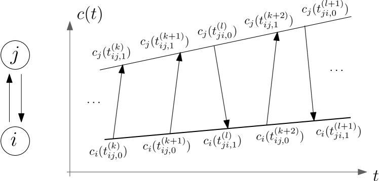
Figure 2: Local clock counters $c_{i}(t)$ and $c_{j}(t)$ of node $i$ and $j$ w.r.t a reference time $t$, and recorded time stamps of the corresponding asymmetric packet exchange.

Following the asymmetric modeling in [19], which is an extension to [8, 16, 17, 18, 21], node pairs $(i,j)\in\mathcal{C}$ exchange packets with time stamps to measure their local clock parameters $\bm{\theta}_{i},\bm{\theta}_{j}$. Node $i$ transmits $K_{ij}\geq 1$ packets to node $j$ and node $j$ transmits $K_{ji}\geq 1$ packets to node $i$. The $k$th “$i\to\!j$” packet (where $k\in\{1,\ldots,K_{ij}\}$) leaves node $i$ at time $t_{ij,0}^{(k)}$ and arrives at node $j$ after a delay $\delta_{ij}^{(k)}$, at measured time

$$t_{ij,1}^{(k)}=t_{ij,0}^{(k)}+\delta_{ij}^{(k)}.$$ (2)

The delay $\delta_{ij}^{(k)}$ is expressed in true time and can be broken up as $\delta_{ij}^{(k)}=\Delta_{ij}+w_{ij}^{(k)}$ [10], where $\Delta_{ij}$ is a deterministic component (related to coding and signal propagation) and $w_{ij}^{(k)}$ is a stochastic component. The nodes record $c_{j}(t_{ij,1}^{(k)})$ and $c_{i}(t_{ij,0}^{(k)})$, which can be related to (2) through (1) as

$$c_{j}(t_{ij,1}^{(k)})\,=\,\psi^{(k)}_{i\to j}(\bm{\theta}_{i},\bm{\theta}_{j},\Delta_{ij})\hskip 0.85358pt+\hskip 0.85358ptw_{ij}^{(k)}\alpha_{j}\,,\vspace*{-1.5mm}$$ (3)

with the deterministic part

$$\psi^{(k)}_{i\to j}(\bm{\theta}_{i},\bm{\theta}_{j},\Delta_{ij})\,\triangleq\,\frac{c_{i}(t_{ij,0}^{(k)})-\beta_{i}}{\alpha_{i}}\alpha_{j}\hskip 0.85358pt+\hskip 0.85358pt\beta_{j}\hskip 0.85358pt+\hskip 0.85358pt\Delta_{ij}\alpha_{j}\,.$$ (4)

A similar relation holds for the packets sent by node $j$ to node $i$, by exchanging $i$ and $j$ in (3). The aggregated measurement of nodes $i$ and $j$ is thus given by $\mathbf{c}_{ij}\triangleq[\mathbf{c}_{i\to j}^{\mathrm{T}}\,\hskip 0.85358pt\hskip 0.85358pt\mathbf{c}_{j\to i}^{\mathrm{T}}]^{\mathrm{T}}\!$, with $\mathbf{c}_{i\to j}\triangleq\big{[}c_{j}(t_{ij,1}^{(1)})\hskip 0.85358pt\cdots\,c_{j}(t_{ij,1}^{(K_{ij})})\big{]}^{\mathrm{T}}\!$ and $\mathbf{c}_{j\to i}\triangleq\big{[}c_{i}(t_{ji,1}^{(1)})$$\cdots\,c_{i}(t_{ji,1}^{(K_{ji})})\big{]}^{\mathrm{T}}\!$. For later use, we also define the (recorded, not measured) time stamp vectors $\tilde{\mathbf{c}}_{i\to j}\triangleq\big{[}c_{i}(t_{ij,0}^{(1)})\cdots c_{i}(t_{ij,0}^{(K_{ij})})\big{]}^{\mathrm{T}}\!$ and $\tilde{\mathbf{c}}_{j\to i}\triangleq\big{[}c_{j}(t_{ji,0}^{(1)})\hskip 0.85358pt\cdots\,c_{j}(t_{ji,0}^{(K_{ji})})\big{]}^{\mathrm{T}}\!$.

\psfrag{s01}[t][t][0.7]{\color[rgb]{0,0,0}\begin{tabular}[]{c}Transmission delay [$\mu s$]\end{tabular}}\psfrag{s02}[b][b][0.7]{\color[rgb]{0,0,0}\begin{tabular}[]{c}Relative occurrence\end{tabular}}\psfrag{s05}[l][l][0.6]{\color[rgb]{0,0,0}Gaussian fit}\psfrag{s06}[l][l][0.6]{\color[rgb]{0,0,0}Measurement}\psfrag{s07}[l][l][0.6]{\color[rgb]{0,0,0}Gaussian fit}\psfrag{s09}{\color[rgb]{0,0,0}\begin{tabular}[]{c}\end{tabular}}\psfrag{s10}{\color[rgb]{0,0,0}\begin{tabular}[]{c}\end{tabular}}\psfrag{x01}[t][t][0.6]{7.4}\psfrag{x02}[t][t][0.6]{7.6}\psfrag{x03}[t][t][0.6]{7.8}\psfrag{x04}[t][t][0.6]{8}\psfrag{x05}[t][t][0.6]{8.2}\psfrag{x06}[t][t][0.6]{8.4}\psfrag{x07}[t][t][0.6]{8.6}\psfrag{v01}[r][r][0.6]{0}\psfrag{v02}[r][r][0.6]{0.02}\psfrag{v03}[r][r][0.6]{0.04}\psfrag{v04}[r][r][0.6]{0.06}\psfrag{v05}[r][r][0.6]{0.08}\psfrag{v06}[r][r][0.6]{0.1}\includegraphics[width=433.62pt]{2_delay_spread_label}

Figure 3: Measurement data and Gaussian fit of the delay $t_{ij,1}^{(k)}-t_{ij,0}^{(k)}=\delta_{ij}^{(k)}=\Delta_{ij}+w_{ij}^{(k)}$.

We model $\Delta_{ij}=T_{c}+T_{f,ij}$ as comprising a hardware related computation time $T_{c}$, and a time of flight $T_{f,ij}$. We further suppose that $\Delta_{ij}=\Delta_{ji}$. Based on the results of a measurement campaign, shown in Fig. 3, with two Texas Instruments ez430-RF2500 evaluation boards, we modeled $w_{ij}^{(k)}\!\!\sim\!\mathcal{N}(0,\sigma^{2}_{w})$, which is congruent with the models from [21, 18, 16, 8]. The evaluated signal corresponds to a time stamping close to the physical layer [22], also often referred to as MAC time stamping [10, 14, 13]. Using this concept, nondeterministic delays from higher layers, such as routing and queuing delays, are eliminated, and the parameters of the delay distribution are assumed to be static.

II-D Network Synchronization

Our goal is to infer the local clock parameters$\alpha_{i}$ and $\beta_{i}$ (or an invertible transformation thereof), based on the measurements and the prior clock information. In the following, sections, we will describe standard approaches to solve this problem, followed by our proposed Bayesian approach.

III State-of-the-Art

In this section, we briefly present a selection of existing synchronization methods for the presented clock and network model. We limit our overview to algorithms that perform skew and phase synchronization based on time stamp exchange in a fully distributed manner, where every node runs the same algorithm. Within this class, we discuss approaches based on consensus [12], alternating direction of multiplier method (ADMM) [11], and loop constrained combination of pairwise estimations [15].

III-A Average TimeSync

Consensus protocols are based on averaging information received from neighbors, and thus have low computational complexity. Moreover, MNs are not considered. A reference time can be introduced, if a single node does not update its local parameters. This modification leads to a decreased convergence speed. In the Average TimeSync (ATS) algorithm from [12], every node has a virtual clock

$$\hat{c}_{i}(c_{i}(t))=\hat{\alpha}_{i}c_{i}(t)+\hat{\beta}_{i}=\hat{\alpha}_{i}\alpha_{i}t+\hat{\alpha}_{i}\beta_{i}+\hat{\beta}_{i},$$

which is controlled by a virtual skew $\hat{\alpha}_{i}$ and a virtual phase $\hat{\beta}_{i}$. By adjusting the virtual skew and phase, ATS assures asymptotic agreement on the virtual clocks $\lim\limits_{t\rightarrow\infty}\hat{c}_{i}(c_{i}(t))=\tau_{v}(t)$, $\forall i\in\mathcal{A}$, where $\tau_{v}(t)$ is a network-wide common time. The algorithm assumes $\delta_{ij}=0$.

III-B ADMM Consensus

In ADMM consensus from [11], relative skews $\alpha_{ij}=\alpha_{i}/\alpha_{j}$ and relative phase offsets $\beta_{ij}=\beta_{i}-\beta_{j}$ are assumed to be available a priori (e.g., from a phase locked loop (PLL), or from an estimation algorithm such as [21]). Then follows a network-wide correction of the local clock parameters in discrete instances $k\Delta T$. Collecting the clock skews in $\mathbf{T}^{(k)}=[\alpha_{1}^{(k)}\Delta T,\ldots,\alpha_{A}^{(k)}\Delta T]^{\mathrm{T}}$, and the clock phases in $\bm{\beta}^{(k)}=[\beta_{1}^{(k)},\ldots,\beta_{A}^{(k)}]^{\mathrm{T}}$, control signals $\mathbf{u}^{(k)}$ and $\mathbf{v}^{(k)}$ are applied as

$$\bm{\beta}^{(k+1)} =\bm{\beta}^{(k)}+\mathbf{T}^{(k)}+\mathbf{u}^{(k)}$$

$$\mathbf{T}^{(k+1)} =\mathbf{T}^{(k)}+\mathbf{v}^{(k)}.$$

The computation of $v_{i}^{(k)}$ at a node $i$ is based on ADMM and requires knowledge of $\alpha_{jk}$ for all nodes $j\in\mathcal{T}_{i},k\in\text{N}(j)$, i.e., from all two-hop neighbors. It can be shown that as $k\to+\infty$, $\mathbf{T}^{(k)}\to\bar{T}\cdot\mathbf{1}_{A,1}$ for some common value $\bar{T}$, where $\mathbf{1}_{k,l}$ denotes a $k\times l$ matrix with all entries equal to one. Finally, agreement on the clock phases is achieved through the control signal $\mathbf{u}^{(k)}$ using average consensus. Although fully distributed and master-free, ADDM consensus requires $I$ inner iterations for offset measurements and outer iterations for the consensus. It further relies on a step size parameter, whose optimal value depends on global network properties.

III-C Loop Constrained Synchronization

In [15], it was observed that for every closed loop $\mathcal{L}$ in the network, it is such that $\sum_{i,j\in\mathcal{L}}\tilde{x}_{ij}=0,$ for $\tilde{x}_{ij}=\beta_{i}-\beta_{j}$ and $\tilde{x}_{ij}=\log(\alpha_{i}/\alpha_{j})$. Using these constraints, the absolute clock values are determined via coordinate descent of the least squares problem [15]

$$\hat{\mathbf{v}}=\arg\min_{\mathbf{v}}\|\mathbf{A}\mathbf{v}-\tilde{\mathbf{x}}\|^{2},$$

where $\mathbf{A}$ is the incidence matrix representing a directed topology, $\mathbf{v}$ the vector of absolute clock parameters (phase or skew) and $\tilde{\mathbf{x}}$ is the collection of offset measurements. In order to find a global optimum, a MN needs to be selected. During the iterations, local estimates on absolute skew and phase are exchanged with all one-hop neighbors.

IV Statistical Models

The above-mentioned algorithms are all non-Bayesian, and thus do not fully exploit all statistical information present in the network. When clock skews are known, fast, distributed Bayesian algorithms were derived in [16]. When clock skews are unknown, the naive extension of [16] would lead to impractical algorithms, due to the complex integrals that need to be computed. In this section, we propose a series of approximations to measurement likelihoods and prior distributions, with the aim of a simple representation of the posterior distribution. Using this simplifications, the maximum a posteriori (MAP) estimate of the clock parameters (or a transformation thereof) can be found with reasonable complexity.

IV-A Likelihood Function

Because of (3) and the statistical properties of $w_{ij}^{(k)}$, the local likelihood function of nodes $i$ and $j$, with $(i,j)\!\in\!\mathcal{C}$, is

$$p(\mathbf{c}_{ij}|\bm{\theta}_{i},\bm{\theta}_{j};\Delta_{ij})$$ (5)

$$\quad=\,G_{ij}\exp\!\left(-\hskip 0.85358pt\frac{\left\|\mathbf{c}_{i\to j}-\bm{\psi}_{i\to j}\right\|^{2}}{2\alpha_{j}^{2}\sigma_{w}^{2}}-\frac{\left\|\mathbf{c}_{j\to i}-\bm{\psi}_{j\to i}\right\|^{2}}{2\alpha_{i}^{2}\sigma_{w}^{2}}\right),$$

where $G_{ij}\triangleq{(2\pi\alpha_{j}^{2}\sigma_{w}^{2})}^{-K_{ij}/2}{(2\pi\alpha_{i}^{2}\sigma_{w}^{2})}^{-K_{ji}/2}$, $\bm{\psi}_{i\to j}\triangleq$$\big{[}\psi^{(1)}_{i\to j}(\bm{\theta}_{i},\bm{\theta}_{j},\Delta_{ij})\,\cdots\,\psi^{(K_{ij})}_{i\to j}(\bm{\theta}_{i},\bm{\theta}_{j},\Delta_{ij})\big{]}^{\mathrm{T}}\!$, and $\bm{\psi}_{j\to i}\triangleq$$\big{[}\psi^{(1)}_{j\to i}(\bm{\theta}_{j},\bm{\theta}_{i},\Delta_{ij})\,\cdots\,\psi^{(K_{ji})}_{j\to i}(\bm{\theta}_{j},\bm{\theta}_{i},\Delta_{ij})\big{]}^{\mathrm{T}}\!$. Since the covariance depends on $\alpha_{i}$ and $\alpha_{j}$ and marginalization over these parameters is not analytically tractable, the direct application of the likelihood function as in [16] for message passing is not straightforward. Moreover, the dependence of the unknown delay $\Delta_{ij}$ does not vanish in the presented distribution. In the following, we propose an approximation of (5) to circumvent these problems. Computing the Fischer information of (5) with respect to $\alpha_{i}$ (and similarly to $\alpha_{j}$), it can be seen that $G_{ij}$ has a smaller contribution than the exponent, as long as $\|\mathbf{t}_{ij,0}\|^{2}+\|\mathbf{t}_{ji,0}+\mathbf{1}\Delta_{ij}\|^{2}\gg K_{ji}\sigma_{w}^{2}$, where $\mathbf{t}_{nm,0}$ is the collection of ${t}_{nm,0}^{(k)},\,k\in\{1,\ldots,K_{nm}\}$. Thus, for practical scenarios we can approximate $G_{ij}\approx\tilde{G}_{ij}\triangleq{(2\pi\sigma_{w}^{2})}^{-K_{ij}/2}{(2\pi\sigma_{w}^{2})}^{-K_{ji}/2}$.

The dependence of the unknown delay $\Delta_{ij}$ can be removed by computing the maximum likelihood estimate of $\Delta_{ij}$ and substituting the estimate back into the likelihood. Taking the logarithm of (5) and setting the derivative with respect to $\Delta_{ij}$ to zero leads to the following estimate

$$\hat{\Delta}_{ij}(\bm{\theta}_{i},\bm{\theta}_{j})=a_{i}\frac{1}{\alpha_{i}}+a_{j}\frac{1}{\alpha_{j}}+b_{ij}\frac{\beta_{i}}{\alpha_{i}}-b_{ij}\frac{\beta_{j}}{\alpha_{j}},$$ (6)

where $a_{i},a_{j},b_{ij}$ are functions of the observations, detailed in Appendix -A. Substituting (6) in (5) and considering the approximation of the normalization constant leads to the following approximate likelihood function

$$\tilde{p} (\mathbf{c}_{ij}|\bm{\vartheta}_{i},\bm{\vartheta}_{j})\propto\exp\left(-\frac{1}{2\sigma_{w}^{2}}\|\mathbf{A}_{ij}\bm{\vartheta}_{i}+\mathbf{B}_{ij}\bm{\vartheta}_{j}\|^{2}\right),$$ (7)

with

$$\mathbf{A}_{ij} \triangleq\begin{bmatrix}-\tilde{\mathbf{c}}_{i\to j}\!\!&\!\!\mathbf{1}_{K_{ij}}\\[1.99168pt] \mathbf{c}_{j\to i}\!\!&\!\!-\mathbf{1}_{K_{ji}}\end{bmatrix}+[a_{i}\ +b_{ij}]\otimes\mathbf{1}_{K_{ij}+K_{ji},1},$$

$$\mathbf{B}_{ij} \triangleq\begin{bmatrix}\mathbf{c}_{i\to j}\!\!&\!\!-\mathbf{1}_{K_{ij}}\\[1.99168pt] -\tilde{\mathbf{c}}_{j\to i}\!\!&\!\!\mathbf{1}_{K_{ji}}\end{bmatrix}+[a_{j}\ -b_{ij}]\otimes\mathbf{1}_{K_{ij}+K_{ji},1},$$

where $\otimes$ denotes the Kronecker product. Note that $\mathbf{A}_{ji}\neq\mathbf{B}_{ij}$, but $\mathbf{A}_{ji}^{\mathrm{T}}\mathbf{A}_{ji}=\mathbf{B}_{ij}^{\mathrm{T}}\mathbf{B}_{ij}$. The approximated likelihood function in (7) no longer contains the delay $\Delta_{ij}$ and can be interpreted as Gaussian in the transformed parameters $\bm{\vartheta}_{i},\bm{\vartheta}_{j}$. As we will see in Section VI, this latter observation has advantages in the algorithm design for distributed parameter estimation since it leads to simpler computation rules.

IV-B Prior Distribution

Since our simplified likelihood function now has a Gaussian form in the transformed clock parameters $\bm{\vartheta}_{i},\bm{\vartheta}_{j}$, we need to select a suitable Gaussian prior so as to end up with a Gaussian posterior distribution.

As MNs induce a reference time in the WN, they have perfect knowledge of their clock parameters, modeled by $p(\bm{\vartheta}_{i})=\delta(\bm{\vartheta}_{i}-\bm{\vartheta}_{i}^{\ast})$, $i\!\in\!\mathcal{M}$, where $\bm{\vartheta}_{i}^{\ast}$ denotes the true transformed clock parameter of MN $i$ and $\delta(\cdot)$ denotes the Dirac delta function. For ANs, clock phases are in the most general case unbounded, and $\nu_{i}\triangleq\beta_{i}/\alpha_{i}$ can be modeled as having an as prior with infinite variance. For bounded intervals, a finite variance can be used. The clock skews depend on various random quantities such as environmental effects, production quality, and supply voltage. Moreover, the skews of correctly working clocks are bounded in intervals close around 1, and we can use the approximation $\lambda_{i}\triangleq 1/\alpha_{i}=1/(1+\varepsilon_{i})\approx 1-\varepsilon_{i}$ [23], where $\varepsilon_{i}\triangleq\alpha_{i}-1$. Finally, for the AN we use the Gaussian prior [20] $p(\bm{\vartheta}_{i})=\mathcal{N}(\bm{\mu}_{\text{p},i},\bm{\Sigma}_{\text{p},i})$, $i\!\in\!\mathcal{A}$, with $\bm{\mu}_{\text{p},i}=[1\;\,0]^{\mathrm{T}}\!$ (note that $\bm{\vartheta}_{i}=[1\;\,0]^{\mathrm{T}}$ would correspond to $\alpha_{i}\!=\!1$ and $\beta_{i}\!=\!0$) and $\bm{\Sigma}_{\text{p},i}={\rm diag}\big{\{}\sigma_{\lambda_{i}}^{2},\sigma_{\nu_{i}}^{2}\big{\}}$. We set $\sigma_{\lambda_{i}}^{2}\!=\sigma_{\alpha_{i}}^{2}$, where $\sigma_{\alpha_{i}}^{2}$ is related to the oscillator specification, and we choose $\sigma_{\nu_{i}}^{2}$ large, since limited prior information on the clock phase $\beta_{i}$ is available.

IV-C Posterior Distribution and Estimator

Putting together the approximate likelihood function from Section IV-A with the prior in the transformed parameters from Section IV-B, we find the following posterior distribution in the transformed parameters

$$\tilde{p}(\bm{\vartheta}|\mathbf{c}) \propto\prod_{i\in\mathcal{A}\cup\mathcal{M}}p(\bm{\vartheta}_{i})\prod_{(i,j)\in\mathcal{C}}\tilde{p}(\mathbf{c}_{ij}|\bm{\vartheta}_{i},\bm{\vartheta}_{j}),$$ (8)

which is a Gaussian distribution in $\bm{\vartheta}$. The inverse covariance matrix $\tilde{\bm{\Sigma}}^{-1}$ of this Gaussian turns out to be highly structured, with block entries (for $i,j\in\mathcal{A}$)

$$\left[\tilde{\bm{\Sigma}}^{-1}\right]_{i,i} =\bm{\Sigma}_{\text{p},i}^{-1}+\sum_{j\in\mathcal{T}_{i}}\frac{1}{\sigma^{2}_{w}}\mathbf{A}_{ij}^{\mathrm{T}}\mathbf{A}_{ij}$$

$$\left[\tilde{\bm{\Sigma}}^{-1}\right]_{i,j} =\left\{\begin{matrix}\frac{1}{\sigma^{2}_{w}}\mathbf{A}_{ij}^{\mathrm{T}}\mathbf{B}_{ij}&\text{for }j\in\mathcal{T}_{i}\\ \mathbf{0}&\text{else.}\end{matrix}\right.$$ (9)

If we are able to marginalize $\tilde{p}(\bm{\vartheta}|\mathbf{c})$ to recover $\tilde{p}(\bm{\vartheta}_{i}|\mathbf{c})$, we can compute the MAP estimate of $\bm{\vartheta}_{i}$, $i\in\mathcal{A}$ as

$$\hat{\bm{\vartheta}}_{i} =\arg\max_{\bm{\vartheta}_{i}}\tilde{p}(\bm{\vartheta}_{i}|\mathbf{c})$$ (10)

$$=\arg\max_{\bm{\vartheta}_{i}}\int\,\tilde{p}(\bm{\vartheta}|\mathbf{c})\,\mathrm{d}\bm{\vartheta}_{\hskip 0.85358pt\bar{i}},$$

where $\bm{\vartheta}_{\hskip 0.85358pt\bar{i}}$ indicates that the integration is over all $\bm{\vartheta}_{j}$ except $\bm{\vartheta}_{i}$. From $\hat{\bm{\vartheta}}_{i}$, we can further determine the clock parameters by $\hat{\alpha}_{i}=1/[\hat{\bm{\vartheta}}_{i}]_{1}$ and $\hat{\beta}_{i}=[\hat{\bm{\vartheta}}_{i}]_{2}/[\hat{\bm{\vartheta}}_{i}]_{1}$, where $[\cdot]_{m}$ extracts the $m$-th element of a vector. Solving this problem in a distributed manner will be the topic of Section VI.

V Bayesian Cramér–Rao Bound

Based on the statistical models from Section IV, it is possible to derive fundamental performance bounds on the quality of estimators. One such bound is the BCRB, which gives a lower bound on the achievable estimation accuracy on $\bm{\theta}_{i}$ [24]. The BCRB is derived based on the Fisher information matrix, assuming known $\Delta_{ij}$ for every link:

$$\mathbf{J} =-\mathbb{E}_{{\bm{\theta},\mathbf{c}}}\begin{bmatrix}\left\{\nabla_{{\bm{\theta}}}\left\{\nabla_{{\bm{\theta}}}[\log p(\bm{\theta}|\mathbf{c};\bm{\Delta})]\right\}^{\mathrm{T}}\right\}\end{bmatrix}$$

$$=-\mathbb{E}_{{\bm{\theta},\mathbf{c}}}\begin{bmatrix}\left\{\nabla_{{\bm{\theta}}}\left\{\nabla_{{\bm{\theta}}}[\log p(\mathbf{c}|\bm{\theta};\bm{\Delta})]\right\}^{\mathrm{T}}\right\}\end{bmatrix}$$

$$\quad-\mathbb{E}_{{\bm{\theta}}}\begin{bmatrix}\left\{\nabla_{{\bm{\theta}}}\left\{\nabla_{{\bm{\theta}}}[\log p(\bm{\theta})]\right\}^{\mathrm{T}}\right\}\end{bmatrix}$$

$$=\mathbb{E}_{{\bm{\theta}}}[\mathbf{J}_{l}]+\mathbb{E}_{{\bm{\theta}}}[\mathbf{J}_{p}],$$ (11)

in which the matrix $\mathbf{J}_{p}$ represents the contribution of the prior information, and is a diagonal matrix with block entries equal to the covariances matrices of the priors. The matrix $\mathbf{J}_{l}$ represents the contribution of the likelihood function $p(\mathbf{c}|\bm{\theta};\Delta)=\mathcal{N}_{\mathbf{c}}(\bm{\mu}_{l},\bm{\Sigma}_{l})$, which is the product of the pairwise functions in (5). It is computed as

$$[\mathbf{J}_{l}]_{i,j}=\frac{\partial\bm{\mu}_{l}^{\mathrm{T}}}{\partial\bm{\theta}_{i}}\bm{\Sigma}_{l}^{-1}\frac{\partial\bm{\mu}_{l}}{\partial\bm{\theta}_{j}}+\frac{1}{2}\text{trace}\left[\bm{\Sigma}_{l}^{-1}\frac{\partial\bm{\Sigma}_{l}}{\partial\bm{\theta}_{i}}\bm{\Sigma}_{l}^{-1}\frac{\partial\bm{\Sigma}_{l}}{\partial\bm{\theta}_{j}}\right]$$ (12)

for $i,j\in\mathcal{A}$. $\mathbf{J}_{l}$ has $2\times 2$ non-zero blocks in the main diagonal and in $i$-th row and $j$-th column when $j\in\mathcal{T}_{i}$. Thus, it will have the same structure as the inverse covariance matrix in (9). Additional details are provided in Appendix -B. Finally, the BCRB on a certain parameter, say the $k$-th parameter in the $2A$-dimensional vector $\bm{\theta}$, is given by

$$\text{BRCB}_{k}=\left[\mathbf{J}^{-1}\right]_{k,k}.$$

VI Distributed Parameter Estimation

To solve the marginalization in (10) in a distributed way, we use approximate inference via message passing on factor graphs. In the following, we describe the factor graph for the synchronization problem and motivate the use of message passing for optimum retrieval of posterior marginals. Finally, we derive two synchronization algorithms.

VI-A Factor Graph

\psfrag{pt01}[t][t][0.65]{\color[rgb]{0,0,0}\begin{tabular}[]{c}\raisebox{6.25958pt}{$\,p(\bm{\vartheta}_{1})$}\end{tabular}}\psfrag{pt02}[t][t][0.65]{\color[rgb]{0,0,0}\begin{tabular}[]{c}\raisebox{6.25958pt}{$\,p(\bm{\vartheta}_{2})$}\end{tabular}}\psfrag{pt03}[t][t][0.65]{\color[rgb]{0,0,0}\begin{tabular}[]{c}\raisebox{6.25958pt}{$\,p(\bm{\vartheta}_{3})$}\end{tabular}}\psfrag{pt4}[t][t][0.65]{\color[rgb]{0,0,0}\begin{tabular}[]{c}\raisebox{6.25958pt}{$\,p(\bm{\vartheta}_{4})$}\end{tabular}}\psfrag{pt5}[t][t][0.65]{\color[rgb]{0,0,0}\begin{tabular}[]{c}\raisebox{6.25958pt}{$\,p(\bm{\vartheta}_{5})$}\end{tabular}}\psfrag{pt12}[b][b][0.65]{\color[rgb]{0,0,0}\begin{tabular}[]{c}\vspace{-0.9mm}{$\,\,\tilde{p}(\mathbf{c}_{12}|\bm{\vartheta}_{1},\bm{\vartheta}_{2})$}\end{tabular}}\psfrag{pt23}[b][b][0.65]{\color[rgb]{0,0,0}\begin{tabular}[]{c}\vspace{-0.9mm}{$\,\,\tilde{p}(\mathbf{c}_{23}|\bm{\vartheta}_{2},\bm{\vartheta}_{3})$}\end{tabular}}\psfrag{pt24}[b][b][0.65]{\color[rgb]{0,0,0}\begin{tabular}[]{c}\vspace{-0.9mm}{$\,\,\tilde{p}(\mathbf{c}_{24}|\bm{\vartheta}_{2},\bm{\vartheta}_{4})$}\end{tabular}}\psfrag{pt25}[b][b][0.65]{\color[rgb]{0,0,0}\begin{tabular}[]{c}\vspace{-1.1mm}{$\hskip 7.11317pt\tilde{p}(\mathbf{c}_{25}|\bm{\vartheta}_{2},\bm{\vartheta}_{5})$}\end{tabular}}\psfrag{pt34}[b][b][0.65]{\color[rgb]{0,0,0}\begin{tabular}[]{c}\vspace{-0.9mm}{$\,\tilde{p}(\mathbf{c}_{34}|\bm{\vartheta}_{3},\bm{\vartheta}_{4})$}\end{tabular}}\psfrag{pt45}[b][b][0.65]{\color[rgb]{0,0,0}\begin{tabular}[]{c}\vspace{-0.9mm}{$\,\,\tilde{p}(\mathbf{c}_{45}|\bm{\vartheta}_{4},\bm{\vartheta}_{5})$}\end{tabular}}\psfrag{t1}[b][b][0.65]{\color[rgb]{0,0,0}\begin{tabular}[]{c}\vspace{-1.4mm}{$\bm{\vartheta}_{1}\hskip 0.85358pt$}\end{tabular}}\psfrag{t2}[b][b][0.65]{\color[rgb]{0,0,0}\begin{tabular}[]{c}\vspace{-1.4mm}{$\hskip 0.85358pt\bm{\vartheta}_{2}$}\end{tabular}}\psfrag{t3}[b][b][0.65]{\color[rgb]{0,0,0}\begin{tabular}[]{c}\vspace{-1.4mm}{$\bm{\vartheta}_{3}$}\end{tabular}}\psfrag{t4}[b][b][0.65]{\color[rgb]{0,0,0}\begin{tabular}[]{c}\vspace{-1.4mm}{$\bm{\vartheta}_{4}$}\end{tabular}}\psfrag{t5}[b][b][0.65]{\color[rgb]{0,0,0}\begin{tabular}[]{c}\vspace{-1.4mm}{$\bm{\vartheta}_{5}$}\end{tabular}}\includegraphics[width=346.89731pt]{6_FG_network_label}

Figure 4: Factor graph of the posterior distribution for a 5 node network with $\mathcal{M}=\{1\}$ and $\mathcal{A}=\{2,3,4,5\}$.

The factor graph associated to the factorization in (8) is found by drawing a variable vertex for every variable (drawn as circles) and a factor/function vertex for every factor (drawn as rectangles). Vertices are connected via edges according to their functional dependencies. The factor graph that corresponds to the connectivity graph in Fig. 1 is depicted in Fig. 4. Note that every variable vertex corresponds to the variables of a physical network node and that every factor vertex corresponds to a measurement link in the physical network. Thus, the structure of the connectivity graph is kept in the factor graph: a tree connectivity remains as tree factor graph, a star connectivity remains as star factor graph, and so on.

Factor graphs are combined with message passing methods in order to compute, e.g., marginal posteriors. Different message passing methods lead to different performance/complexity trade-offs. A framework to compare message passing method is found through variational free energy minimization.

VI-B Energy Minimization for Marginal Retrieval

Our goal is to find practical methods to determine, exactly or approximately, the marginals from (10). From [26], one strategy is to minimize the variational free energy for a positive function $b(\bm{\vartheta})$ approximating $\tilde{p}(\bm{\vartheta}|\mathbf{c})$:

$$b^{*}(\cdot)=\arg\min_{b(\cdot)}\int b(\bm{\vartheta})\,\log\frac{b(\bm{\vartheta})}{\tilde{p}(\bm{\vartheta}|\mathbf{c})}\,\mathrm{d}\bm{\vartheta}.$$ (13)

As algorithm designers, we can impose structure to the function $b(\bm{\vartheta})$ to allow efficient solving of (13). We will consider two classes of functions: (i) the Bethe method, in which $b(\bm{\vartheta})$ is constrained to be a product of factors of the form $b_{i}(\bm{\vartheta}_{i})$ and $b_{ij}(\bm{\vartheta}_{i},\bm{\vartheta}_{j})$; and (ii) the mean field method, which constrains $b(\bm{\vartheta})$ to be of the form $b(\bm{\vartheta})=\prod_{i}b_{i}(\bm{\vartheta}_{i})$. Minimizing (13) subject to the constraints imposed by the approximations, leads to the message passing rules [26]. The message passing rules turn out to be the belief propagation (BP) equations for class (i) and the mean field (MF) equations for class (ii).

In the following we use the shorthand ${p}_{ij}$ for $\tilde{p}(\mathbf{c}_{ij}|\bm{\vartheta}_{i},\bm{\vartheta}_{j})$. Furthermore, since the approximated joint posterior distribution in (8) is Gaussian in $\bm{\vartheta}$, we consider only messages that are Gaussian in $\bm{\vartheta}$.

VI-C Synchronization by Message Passing

Above, we introduced two message passing schemes, BP and MF. By applying both, we find two synchronization algorithms where network nodes cooperate by the exchange of messages. We now present the algorithms in detail, and discuss their salient properties. A unified view of the message passing is offered in Fig. 5.

\psfrag{ptij}[b][b][0.8]{\color[rgb]{0,0,0}\begin{tabular}[]{c}\vspace{-0.9mm}{$\,\,\tilde{p}(\mathbf{c}_{ij}|\bm{\vartheta}_{i},\bm{\vartheta}_{j})$}\end{tabular}}\psfrag{ti}[b][b][0.8]{\color[rgb]{0,0,0}\begin{tabular}[]{c}{\vspace{-1.2mm} $\bm{\vartheta}_{i}\hskip 0.85358pt$}\end{tabular}}\psfrag{tj}[b][b][0.8]{\color[rgb]{0,0,0}\begin{tabular}[]{c}{\vspace{-0.7mm} \hskip 0.85358pt$\bm{\vartheta}_{j}$}\end{tabular}}\psfrag{msg1j}[l][c][0.8]{\color[rgb]{0,0,0} \vspace{5mm} \begin{tabular}[]{lr}BP: $m_{\bm{\vartheta}_{j}\to p_{ij}}\hskip 14.22636pt$&\eqref{eq:BPmsg_pij_in}\\ MF: $b_{\bm{\vartheta}_{j}}\hskip 14.22636pt$&\eqref{eq:MF_marg}\end{tabular}}\psfrag{msg1i}[l][c][0.8]{\color[rgb]{0,0,0} \vspace{7mm} \begin{tabular}[]{lr}BP: $m_{\bm{\vartheta}_{i}\to p_{ij}}\hskip 14.22636pt$&\eqref{eq:BPmsg_pij_in}\\ MF: $b_{\bm{\vartheta}_{i}}\hskip 14.22636pt$&\eqref{eq:MF_marg}\end{tabular}}\psfrag{msg2j}[l][c][0.8]{\color[rgb]{0,0,0} \vspace{7mm} \begin{tabular}[]{lr}$m_{\bm{p_{ij}\to\vartheta}_{j}}\hskip 14.22636pt$&\eqref{eq:BPmsg_thetai_in} or \eqref{eq:MFmsg_thetai_in}\end{tabular}}\psfrag{msg2i}[l][c][0.8]{\color[rgb]{0,0,0} \vspace{7mm} \begin{tabular}[]{lr}$m_{\bm{p_{ij}\to\vartheta}_{i}}\hskip 14.22636pt$&\eqref{eq:BPmsg_thetai_in} or \eqref{eq:MFmsg_thetai_in}\end{tabular}}\psfrag{ci}[l][c][0.8]{\color[rgb]{0.5,0.5,0.5}\begin{tabular}[]{c} \vspace{-1mm} Computed by node\leavevmode\nobreak\ $i$\end{tabular}}\psfrag{cj}[l][c][0.8]{\color[rgb]{0.5,0.5,0.5}\begin{tabular}[]{c} \vspace{-1mm} Computed by node\leavevmode\nobreak\ $j$\end{tabular}}\includegraphics[width=303.53267pt]{6_msg_exchange_label}

Figure 5: Messages between a node pair $i,j$ of a general network. Since the measurements are shared, both nodes have access to the same function vertex.

VI-C1 Belief Propagation

The BP message from a factor vertex $p_{ij}$ to a variable vertex $\bm{\vartheta}_{i}$ is given by [27, Eq. (6)]

$$m_{{p}_{ij}\rightarrow\bm{\vartheta}_{i}}(\bm{\vartheta}_{i}) =\int{p}_{ij}(\bm{\vartheta}_{i},\bm{\vartheta}_{j})\ m_{\bm{\vartheta}_{j}\rightarrow{p}_{ij}}(\bm{\theta}_{j}^{\prime})\,\mathrm{d}\bm{\theta}_{j}^{\prime}$$

$$\propto\mathcal{N}_{\bm{\vartheta}_{i}}\left(\bm{\mu}_{\text{in},ij},\bm{\Sigma}_{\text{in},ij}\right),$$ (14)

while the BP message from a variable vertex $\bm{\vartheta}_{i}$ to a factor vertex $p_{ij}$ is given by [27, Eq. (5)]

$$m_{\bm{\vartheta}_{i}\rightarrow{p}_{ij}}(\bm{\vartheta}_{i}) =p(\bm{\vartheta}_{i})\prod_{k\in\{\mathcal{T}_{i}\backslash j\}}\ m_{{p}_{ik}\rightarrow\bm{\vartheta}_{i}}(\bm{\vartheta}_{i})$$

$$\propto\mathcal{N}_{\bm{\vartheta}_{i}}\left(\bm{\mu}_{\text{ext},ij},\bm{\Sigma}_{\text{ext},ij}\right),$$ (15)

where we use the index “in” for intrinsic and “ext” for extrinsic with respect to a variable vertex. As depicted in Fig. 5, each network node $i$ corresponding to the variable vertex $\bm{\vartheta}_{i}$ needs to compute its intrinsic and extrinsic message. Furthermore, note that for BP, the extrinsic message $m_{\bm{\vartheta}_{i}\rightarrow{p}_{ij}}$ has to be determined separately for every node $j\in\mathcal{T}_{i}$. If the neighboring node is an agent, $j\in\mathcal{T}_{i}\cap\mathcal{A}$, the parameter updates (for detailed derivations, see Appendix -C) of (14) are

$$\mathbf{Q} =\mathbf{A}_{ij}^{\mathrm{T}}\mathbf{B}_{ij}\left(\mathbf{B}_{ij}^{\mathrm{T}}\mathbf{B}_{ij}+\sigma_{w}^{2}\bm{\Sigma}_{\text{ext},ji}^{-1}\right)^{-1}$$

$$\bm{\Sigma}_{\text{in},ij}^{-1} =\frac{1}{\sigma_{w}^{2}}\mathbf{A}_{ij}^{\mathrm{T}}\mathbf{A}_{ij}-\frac{1}{\sigma_{w}^{2}}\mathbf{Q}\,\mathbf{B}_{ij}^{\mathrm{T}}\mathbf{A}_{ij}$$ (16a)

$$\bm{\Sigma}_{\text{in},ij}^{-1}\bm{\mu}_{\text{in},ij} =-\mathbf{Q}\,\bm{\Sigma}_{\text{ext},ji}^{-1}\bm{\mu}_{\text{ext},ji},$$ (16b)

and if the neighboring node is a master, $j\in\mathcal{T}_{i}\cap\mathcal{M}$

$$\bm{\Sigma}_{\text{in},ij}^{-1} =\frac{1}{\sigma_{w}^{2}}\mathbf{A}_{ij}^{\mathrm{T}}\mathbf{A}_{ij}$$ (17a)

$$\bm{\Sigma}_{\text{in},ij}^{-1}\bm{\mu}_{\text{in},ij} =-\frac{1}{\sigma_{w}^{2}}\mathbf{A}_{ij}^{\mathrm{T}}\mathbf{B}_{ij}\bm{\mu}_{\text{ext},ji}.$$ (17b)

The parameter updates of (15) are

$$\bm{\Sigma}_{\text{ext},ij}^{-1} =\bm{\Sigma}_{\text{p},i}^{-1}+\sum_{k\in\{\mathcal{T}_{i}\backslash j\}}\bm{\Sigma}_{\text{in},ki}^{-1}$$ (18a)

$$\bm{\Sigma}_{\text{ext},ij}^{-1}\bm{\mu}_{\text{ext},ij} =\bm{\Sigma}_{\text{p},i}^{-1}\bm{\mu}_{\text{p},i}+\sum_{k\in\{\mathcal{T}_{i}\backslash j\}}\bm{\Sigma}_{\text{in},ki}^{-1}\bm{\mu}_{\text{in},ki}.$$ (18b)

The approximate marginal is obtained by

$$b_{i}(\bm{\vartheta}_{i}) \propto p(\bm{\vartheta}_{i})\prod_{k\in\mathcal{T}_{i}}\ m_{{p}_{ik}\rightarrow\bm{\vartheta}_{i}}(\bm{\vartheta}_{i})$$

$$\propto\mathcal{N}_{\bm{\vartheta}_{i}}\left(\bm{\mu}_{i},\bm{\Sigma}_{i}\right).$$ (19)

The parameters of the marginal belief (19) are computed from the parameters in (18a) and (18b), but with the additional summation over $j$.

In the communication between two connected nodes $i$ and $j$ as in Fig. 5, node $i$ transmits $m_{\bm{\vartheta}_{i}\rightarrow{p}_{ij}}$ to $j$ and vice versa. The receiving node then computes its intrinsic message to the variable vertex (e.g., node $j$ computes $m_{{p}_{ij}\rightarrow\bm{\vartheta}_{j}}$). As a node $i$ has evaluated the intrinsic messages from all its neighbors, it can determine again its extrinsic messages. After $I$ iterations, every node $i$ computes the marginal belief $b_{j}(\bm{\vartheta}_{j})$ and thereof the MAP estimates of its clock parameters.

VI-C2 Mean Field

The MF message from a factor vertex $p_{ij}$ to a variable vertex $\bm{\vartheta}_{i}$ is given by [28, Eq. (14)]

$$m_{{p}_{ij}\rightarrow\bm{\vartheta}_{i}}(\bm{\vartheta}_{i}) =\exp\left(\int\log\left({p}_{ij}(\bm{\vartheta}_{i},\bm{\vartheta}_{j})\right)\ b_{j}(\bm{\vartheta}_{j})\,\mathrm{d}\bm{\theta}_{j}^{\prime}\right)$$

$$\propto\mathcal{N}_{\bm{\vartheta}_{i}}\left(\bm{\mu}_{\text{in},ij},\bm{\Sigma}_{\text{in},ij}\right),$$ (20)

and the message from a variable vertex $\bm{\vartheta}_{i}$ to a factor vertex $p_{ij}$ is given by the belief [28, Eq. (16)]

$$b_{i}(\bm{\vartheta}_{i}) \propto p(\bm{\vartheta}_{i})\prod_{k\in\mathcal{T}_{i}}\ m_{{p}_{ik}\rightarrow\bm{\vartheta}_{i}}(\bm{\vartheta}_{i})$$

$$\propto\mathcal{N}_{\bm{\vartheta}_{i}}\left(\bm{\mu}_{i},\bm{\Sigma}_{i}\right).$$ (21)

The corresponding parameter updates (for detailed derivations, see Appendix -D) are

$$\bm{\Sigma}_{\text{in},ij}^{-1} =\frac{1}{\sigma_{w}^{2}}\mathbf{A}_{ij}^{\mathrm{T}}\mathbf{A}_{ij}$$ (22a)

$$\bm{\Sigma}_{\text{in},ij}^{-1}\bm{\mu}_{\text{in},ij} =-\frac{1}{\sigma_{w}^{2}}\mathbf{A}_{ij}^{\mathrm{T}}\mathbf{B}_{ij}\bm{\mu}_{j}$$ (22b)

and

$$\bm{\Sigma}_{i}^{-1} =\bm{\Sigma}_{\text{p},i}^{-1}+\sum_{k\in\mathcal{T}_{i}}\bm{\Sigma}_{\text{in},ki}^{-1}$$ (23a)

$$\bm{\Sigma}_{i}^{-1}\bm{\mu}_{i} =\bm{\Sigma}_{\text{p},i}^{-1}\bm{\mu}_{\text{p},i}+\sum_{k\in\mathcal{T}_{i}}\bm{\Sigma}_{\text{in},ki}^{-1}\bm{\mu}_{\text{in},ki}.$$ (23b)

For MF, two connected nodes $(i,j)$ only need to exchange their beliefs instead of extrinsic information (see Fig. 5). Since the same information is sent to all neighbors, this can also be performed in a broadcast scheme. From the belief, the receiver can then compute the intrinsic message (20).

VI-D Convergence

VI-D1 Mean Field

MF optimizes node potentials, and for successive message updates, it is known to converge [29, Theorem 11.10] as the energy functional is monotonically decreasing and bounded. In Gaussian models, depending on the message ordering, MF converges to the true mean vectors [30, pp.136].

VI-D2 Belief Propagation

BP optimizes node and edge potentials, and convergence in cyclic graphs depends on the underlying system. For Gaussian models, several sufficient conditions based on analysis of message propagation on the computation tree exist. These include diagonal dominance [31] or walk-summability [32], and FG normalizabilitiy [33], all of which can be evaluated via the information matrix (9). In the following, we will prove the convergence of the proposed algorithms based on FG normalizabilitiy, which is a variant of the walk-sum interpretation

Theorem 1

The variances of the proposed BP algorithm converge for connected networks without MNs, if each node has a prior with finite variance on skew and phase.

Proof:

See Appendix -E1. ∎

Theorem 2

The variances of the proposed BP algorithm converge for all connected networks with at least one MN.

Proof:

See Appendix -E2. ∎

Once the variances converge, the mean updates follow a linear system. As shown in [33], the convergence to the correct means can be forced by sufficient damping. In our numerical analysis, we did not encounter a single case where damping was necessary.

VI-E Scheduling and Implementation Aspects

In this section, we discuss message scheduling and ways to efficiently combine timing information exchange and message passing in real applications.

We consider a general topology as in Fig. 4. Every node $i\in\mathcal{A}$ runs the same algorithm, and computes the message parameters to/from the function vertices as depicted in Fig. 5. Therefore, the node requires $m_{\bm{\vartheta}_{j}\rightarrow{p}_{ij}}(\bm{\vartheta}_{j})$ to compute $m_{{p}_{ij}\rightarrow\bm{\vartheta}_{i}}(\bm{\vartheta}_{i})$. Together with the prior information, the node then computes the outgoing message $m_{\bm{\vartheta}_{i}\rightarrow{p}_{ij}}(\bm{\vartheta}_{i})$, which is sent to neighbor $j$ for the next iteration. In order to start this procedure, all $m_{\bm{\vartheta}_{j}\rightarrow p_{ji}}(\bm{\vartheta}_{j})$ in the factor graph have to be initialized. This can be done by setting them to uniform distributions, with zero mean value and infinite covariance.

In general, all nodes work in parallel for all iterations. As discussed in Sec. VI-D, MF convergence guarantees are only available for specific schedules. Since these are generally not practical in real applications, we propose a mixed serial/parallel MF schedule as follows: A node only updates its beliefs if information from a MN has propagated via any path to the node. Hence, in the first iteration only MNs $m\in\mathcal{M}$ propagate messages. In the second iteration, also their neighbors $j\in\mathcal{T}_{m}$ will send messages, in the third their neighbors’ neighbors and so on. The schedule is serial in the initial information propagation, and a compromise of the successive message updates and a parallel schedule. A similar schedule can be applied for MF if no MNs are available. Thereby, only nodes in the neighborhood of the AN which initializes the synchronization start to join the protocol. In this case, the initializing node also adjusts its clock parameters.

Finally, our derivations were based on the assumption that measurements were collected first, and then message passing was carried out. Since both phases rely on the exchange of packets between nodes, it is possible to combine them, thereby increasing the number of measurements as message passing iterations progress. Such piggybacking is beneficial in real applications. In order to successfully start the algorithm, a minimum number of measurement packets has to be exchanged between every node pair to provide initial timing information. This is due to the required matrix inversions in the message parameter computations.

Table I: Complexity per estimation update

	Num. Operations	Num. Transm.
MF	once: $6\,|\mathcal{T}_{i}|\,(K_{ij}+K_{ji})\,O$	$K_{ij}$
	$14\,|\mathcal{T}_{i}|\,O$	1
BP	once: $9\,|\mathcal{T}_{i}|\,(K_{ij}+K_{ji})\,O$	$K_{ij}$
	$(5\,|\mathcal{T}_{i}|^{2}+35\,|\mathcal{T}_{i}|\,)\,O$	1
ATS [12]	$21\,|\mathcal{T}_{i}|\,O$	1
ADMM [11]	$9I\,|\mathcal{T}_{i}|O$	$2I$
LC [15]	$29\,|\mathcal{T}_{i}|\,O$	$2$

VI-F Comparison with State-of-the-Art Algorithms

We will now describe the main similarities and differences of BP and MF to the previously described state-of-the-art algorithms from Section III. We will use the shorthand: ATS is Average TimeSync from [12], ADMM is the method proposed in [11], and LC is the loop constraint method from [15].

VI-F1 Complexity

We compare the complexity per node $i\in\mathcal{A}$ with the number of operations needed per estimation update. In Table I we provide a complexity estimate, where the operations $+,-,*,\sqrt{\cdot},\log$ and $\exp$ are equated with by one operation cost $O$, and only factors containing the number of neighbors $|\mathcal{T}_{i}|$ are considered. As MF and BP require a measurement phase, they must additionally transmit measurement packets and then compute matrix products of $\mathbf{A}_{ij}$ and $\mathbf{B}_{ij}$. For ADMM, $I=1$ inner iterations and the estimation of $\alpha_{ij}$ using a PLL were considered. It can be seen that all methods scale linearly with the number of neighbors $|\mathcal{T}_{i}|$, only BP scales quadratically. ADMM has the lowest complexity per transmitted packet, followed by LC, MF, ATS, and BP. For a full complexity analysis, the total number of transmitted packets upon convergence must be considered. This is done in Sec. VII-C.

VI-F2 Delay sensitivity

Propagation delays $\delta_{ij}$ influence the performance of the algorithm if not considered correctly. BP, MF and LC algorithms consider the delay as symmetric and unknown. Moreover, in ADMM and in ATS it is disregarded and equated to zero. Thus, the accuracy of ADMM and ATS is decreased if $\delta_{ij}$ increases, i.e., by additional deterministic delays.

VI-F3 Master nodes

As discussed at the convergence section, BP and MF can operate with and without MNs. LC, ATS and ADMM do not consider the use of a time reference.

VI-F4 Broadcast protocols

For ATS, LC, and MF, a node $i$ needs to pass identical values to all neighbors $j\in\mathcal{T}_{i}$. ADMM and BP have destination-specific messages. In principle, this can also be accomplished by broadcast messages, when stacking the information to all neighbors in one packet. Thus all algorithms can be used with broadcast protocols, however ADMM and BP have higher bandwidth requirements.

The remaining question regarding the estimation accuracy is addressed in the following section, where a superior behavior of BP and MF is observed.

VII Numerical Analysis

\psfrag{s01}[t][t][0.8]{\color[rgb]{0,0,0}\begin{tabular}[]{c}$x$-position [m]\end{tabular}}\psfrag{s02}[b][b][0.8]{\color[rgb]{0,0,0}\begin{tabular}[]{c}$y$-position [m]\end{tabular}}\psfrag{x01}[t][t][0.7]{0}\psfrag{x02}[t][t][0.7]{250}\psfrag{x03}[t][t][0.7]{500}\psfrag{x04}[t][t][0.7]{750}\psfrag{x05}[t][t][0.7]{1000}\psfrag{v01}[r][r][0.7]{0}\psfrag{v02}[r][r][0.7]{250}\psfrag{v03}[r][r][0.7]{500}\psfrag{v04}[r][r][0.7]{750}\psfrag{v05}[r][r][0.7]{1000}\includegraphics[width=303.53267pt]{7_Network_label}

Figure 6: Randomly connected network with $M=1$ (circle) and $A=25$ (cross).

VII-A Simulation Settings

If not specified otherwise, we use the delay and noise setting from the measurements in Fig. 3. In particular, the noise standard deviation is $\sigma_{w}=93\,$ns and the deterministic delay $\Delta_{ij}=T_{c}+T_{f,ij}$ comprises a computational time $T_{c}=\linebreak 7.6\,\mu\mathrm{s}$ and the flight time $T_{f,ij}=d_{ij}/v$, where $d_{ij}$ is the distance between nodes $i$ and $j$, and $v$ is the speed of light. Simulations were carried out on randomly generated topologies with 26 nodes, as depicted in Fig. 6. We further select $K_{ij}=K_{ji}$ between all node pairs, where a measure-ment from node $i$ to node $j$ is always followed with a measurement from node $j$ to node $i$. The time between two subsequent measurements is set to $10\,$ms. The clock skews are drawn from a normal distribution corresponding to a 100 ppm specification,$\,\alpha_{i}\!\sim\!\mathcal{N}(1,10^{-8})$, which represents the prior distribution. The clock phases are drawn from a uniform distribution in the interval $[-10,+10]\,$s, where the Gaussian prior was specified with zero mean and a standard deviation of $\sigma_{\beta,i}=5.8\,$s. In the following, we will use the root mean square error as performance measure, denoted by “RMSE of phase” and “RMSE of skew”. Since not all competing algorithms rely on a MN, the RMSE to the true clock parameters is not a meaningful measure in a direct comparison. Thus, for algorithms not supporting MNs, the RMSE is evaluated with respect to the network’s mean error of skew and phase.

VII-B Study of BP and MF Synchronization

VII-B1 Convergence Rate

\psfrag{s02}[b][b][0.7]{\color[rgb]{0,0,0}\begin{tabular}[]{c}RMSE on phase [ms]\end{tabular}}\psfrag{s05}[l][l]{\color[rgb]{0,0,0}BCRB}\psfrag{s06}[l][l][0.6]{\color[rgb]{0,0,0}MF}\psfrag{s07}[l][l][0.6]{\color[rgb]{0,0,0}BP}\psfrag{s08}[l][l][0.6]{\color[rgb]{0,0,0}BCRB}\psfrag{s10}{\color[rgb]{0,0,0}\begin{tabular}[]{c}\end{tabular}}\psfrag{s11}{\color[rgb]{0,0,0}\begin{tabular}[]{c}\end{tabular}}\psfrag{s12}[t][t][0.7]{\color[rgb]{0,0,0}\begin{tabular}[]{c}Number of message iterations\end{tabular}}\psfrag{s13}[b][b][0.7]{\color[rgb]{0,0,0}\begin{tabular}[]{c}RMSE on skew [ppm]\end{tabular}}\psfrag{x01}[t][t]{0}\psfrag{x02}[t][t]{0.1}\psfrag{x03}[t][t]{0.2}\psfrag{x04}[t][t]{0.3}\psfrag{x05}[t][t]{0.4}\psfrag{x06}[t][t]{0.5}\psfrag{x07}[t][t]{0.6}\psfrag{x08}[t][t]{0.7}\psfrag{x09}[t][t]{0.8}\psfrag{x10}[t][t]{0.9}\psfrag{x11}[t][t]{1}\psfrag{x28}[t][t][0.6]{0}\psfrag{x29}[t][t][0.6]{1}\psfrag{x30}[t][t][0.6]{2}\psfrag{x31}[t][t][0.6]{3}\psfrag{x32}[t][t][0.6]{4}\psfrag{x33}[t][t][0.6]{5}\psfrag{x34}[t][t][0.6]{6}\psfrag{x35}[t][t][0.6]{7}\psfrag{x36}[t][t][0.6]{8}\psfrag{x37}[t][t][0.6]{9}\psfrag{x15}[t][t][0.6]{7}\psfrag{x16}[t][t][0.6]{8}\psfrag{x17}[t][t][0.6]{9}\psfrag{x18}[t][t][0.6]{0}\psfrag{x19}[t][t][0.6]{1}\psfrag{x20}[t][t][0.6]{2}\psfrag{x21}[t][t][0.6]{3}\psfrag{x22}[t][t][0.6]{4}\psfrag{x23}[t][t][0.6]{5}\psfrag{x24}[t][t][0.6]{6}\psfrag{x25}[t][t][0.6]{7}\psfrag{x26}[t][t][0.6]{8}\psfrag{x27}[t][t][0.6]{9}\psfrag{x12}[t][t][0.6]{7}\psfrag{x13}[t][t][0.6]{8}\psfrag{x14}[t][t][0.6]{9}\psfrag{v01}[r][r]{0}\psfrag{v02}[r][r]{0.1}\psfrag{v03}[r][r]{0.2}\psfrag{v04}[r][r]{0.3}\psfrag{v05}[r][r]{0.4}\psfrag{v06}[r][r]{0.5}\psfrag{v07}[r][r]{0.6}\psfrag{v08}[r][r]{0.7}\psfrag{v09}[r][r]{0.8}\psfrag{v10}[r][r]{0.9}\psfrag{v11}[r][r]{1}\psfrag{v12}[r][r][0.6]{$0.05$}\psfrag{v13}[r][r][0.6]{$0.1$}\psfrag{v14}[r][r][0.6]{$0.15$}\psfrag{v15}[r][r][0.6]{$0.2$}\psfrag{v16}[r][r][0.6]{$0.25\,10^{-4}$}\psfrag{v17}[r][r][0.6]{$0.5\,10^{-4}$}\psfrag{v18}[r][r][0.6]{$0.74\,10^{-4}$}\psfrag{v19}[r][r][0.6]{$10^{-4}$}\psfrag{v20}[r][r][0.6]{$10^{-2}$}\psfrag{v21}[r][r][0.6]{$1$}\psfrag{v22}[r][r][0.6]{$10^{2}$}\psfrag{v23}[r][r][0.6]{$10^{-5}$}\psfrag{v24}[r][r][0.6]{$10^{-2}$}\psfrag{v25}[r][r][0.6]{$10$}\psfrag{v26}[r][r][0.6]{$10^{4}$}\psfrag{ypower3}[Bl][Bl]{}\includegraphics[width=390.25534pt]{7_study_Iter_label2}

Figure 7: Convergence of parameter estimates with $K_{ij}=K_{ji}=20$.

In Fig. 7, we show the BP and MF mean square error of the phase and skew estimates as a function of the iteration index. For the topology in Fig. 6, we observed that both algorithms converge after a number of iterations that correspond to the largest multi-hop distance of a node to a master node. Furthermore, both algorithms converge to the same values. The gap between estimation accuracy and BCRB arises due to the prior uncertainty of the clock phases.

\psfrag{s13}[b][b][0.7]{\color[rgb]{0,0,0}\begin{tabular}[]{c}RMSE on skew [ppm]\end{tabular}}\psfrag{s05}[l][l]{\color[rgb]{0,0,0}asdddd}\psfrag{s06}[l][l][0.6]{\color[rgb]{0,0,0}MF - s}\psfrag{s07}[l][l][0.6]{\color[rgb]{0,0,0}MF - p}\psfrag{s08}[l][l][0.6]{\color[rgb]{0,0,0}BP}\psfrag{s10}{\color[rgb]{0,0,0}\begin{tabular}[]{c}\end{tabular}}\psfrag{s11}{\color[rgb]{0,0,0}\begin{tabular}[]{c}\end{tabular}}\psfrag{s12}[t][t][0.7]{\color[rgb]{0,0,0}\begin{tabular}[]{c}Number of message iterations\end{tabular}}\psfrag{s02}[b][b][0.7]{\color[rgb]{0,0,0}\begin{tabular}[]{c}RMSE on phase [ms]\end{tabular}}\psfrag{x01}[t][t]{0}\psfrag{x02}[t][t]{0.1}\psfrag{x03}[t][t]{0.2}\psfrag{x04}[t][t]{0.3}\psfrag{x05}[t][t]{0.4}\psfrag{x06}[t][t]{0.5}\psfrag{x07}[t][t]{0.6}\psfrag{x08}[t][t]{0.7}\psfrag{x09}[t][t]{0.8}\psfrag{x10}[t][t]{0.9}\psfrag{x11}[t][t]{1}\psfrag{x12}[t][t][0.6]{0}\psfrag{x13}[t][t][0.6]{20}\psfrag{x14}[t][t][0.6]{40}\psfrag{x15}[t][t][0.6]{60}\psfrag{x16}[t][t][0.6]{0}\psfrag{x17}[t][t][0.6]{20}\psfrag{x18}[t][t][0.6]{40}\psfrag{x19}[t][t][0.6]{60}\psfrag{x20}[t][t][0.6]{0}\psfrag{x21}[t][t][0.6]{100}\psfrag{x22}[t][t][0.6]{200}\psfrag{x23}[t][t][0.6]{300}\psfrag{x24}[t][t][0.6]{400}\psfrag{x25}[t][t][0.6]{500}\psfrag{x26}[t][t][0.6]{600}\psfrag{x27}[t][t][0.6]{700}\psfrag{x28}[t][t][0.6]{800}\psfrag{x29}[t][t][0.6]{900}\psfrag{x30}[t][t][0.6]{0}\psfrag{x31}[t][t][0.6]{100}\psfrag{x32}[t][t][0.6]{200}\psfrag{x33}[t][t][0.6]{300}\psfrag{x34}[t][t][0.6]{400}\psfrag{x35}[t][t][0.6]{500}\psfrag{x36}[t][t][0.6]{600}\psfrag{x37}[t][t][0.6]{700}\psfrag{x38}[t][t][0.6]{800}\psfrag{x39}[t][t][0.6]{900}\psfrag{v01}[r][r]{0}\psfrag{v02}[r][r]{0.1}\psfrag{v03}[r][r]{0.2}\psfrag{v04}[r][r]{0.3}\psfrag{v05}[r][r]{0.4}\psfrag{v06}[r][r]{0.5}\psfrag{v07}[r][r]{0.6}\psfrag{v08}[r][r]{0.7}\psfrag{v09}[r][r]{0.8}\psfrag{v10}[r][r]{0.9}\psfrag{v11}[r][r]{1}\psfrag{v12}[t][t][0.6]{$10^{-4}\,$ }\psfrag{v13}[t][t][0.6]{$10^{-2}\,$ }\psfrag{v14}[t][t][0.6]{$1$}\psfrag{v15}[t][t][0.6]{$10^{-2}\,$ }\psfrag{v16}[t][t][0.6]{$1$}\psfrag{v17}[t][t][0.6]{$10^{2}$}\psfrag{v18}[t][t][0.6]{$10^{4}$}\psfrag{v19}[t][t][0.6]{$10^{-4}\,$ }\psfrag{v20}[t][t][0.6]{$10^{-2}\,$ }\psfrag{v21}[t][t][0.6]{$1$}\psfrag{v22}[t][t][0.6]{$10^{2}$}\psfrag{v23}[t][t][0.6]{$10^{4}$}\psfrag{v24}[t][t][0.6]{$10^{-2}$ }\psfrag{v25}[t][t][0.6]{$1$}\psfrag{v26}[t][t][0.6]{$10^{2}$}\psfrag{v27}[t][t][0.6]{$10^{4}$}\includegraphics[width=390.25534pt]{7_study_noMaster_label2}

Figure 8: Convergence of clock parameters without MN, every node pair with $K_{ij}=K_{ji}=20$.

As indicated by the proof of convergence, MF and BP do not require a MN for convergence if prior information with finite variances is available on all parameters. The convergence without MN is depicted in Fig. 8, where BP uses a parallel schedule , and two schedules for MF are considered: “MF - p” is a parallel schedule, and “MF - s” is the serial schedule from Sec. VI-E. It can be observed that all algorithms converge, whereas “MF - s” has a significant higher convergence speed than “MF - p”.

VII-B2 Impact of Measurements

\psfrag{s01}[b][b][0.7]{\color[rgb]{0,0,0}\begin{tabular}[]{c}RMSE on phase [ms]\end{tabular}}\psfrag{s05}[l][l]{\color[rgb]{0,0,0}asddddd}\psfrag{s06}[l][l][0.6]{\color[rgb]{0,0,0}MF}\psfrag{s07}[l][l][0.6]{\color[rgb]{0,0,0}BP}\psfrag{s08}[l][l][0.6]{\color[rgb]{0,0,0}BCRB}\psfrag{s10}{\color[rgb]{0,0,0}\begin{tabular}[]{c}\end{tabular}}\psfrag{s11}{\color[rgb]{0,0,0}\begin{tabular}[]{c}\end{tabular}}\psfrag{s12}[t][t][0.7]{\color[rgb]{0,0,0}\begin{tabular}[]{c}Number of measurements\end{tabular}}\psfrag{s13}[b][b][0.7]{\color[rgb]{0,0,0}\begin{tabular}[]{c}RMSE on skew [ppm]\end{tabular}}\psfrag{x01}[t][t][0.6]{$1$}\psfrag{x02}[t][t][0.6]{$10$}\psfrag{x03}[t][t][0.6]{$100$}\psfrag{x04}[t][t][0.6]{$1000$}\psfrag{x05}[t][t][0.6]{$1$}\psfrag{x06}[t][t][0.6]{$10$}\psfrag{x07}[t][t][0.6]{$100$}\psfrag{x08}[t][t][0.6]{$1000$}\psfrag{v07}[r][r][0.6]{$10^{-5}$}\psfrag{v08}[r][r][0.6]{$10^{-4}$}\psfrag{v09}[r][r][0.6]{$10^{-3}$}\psfrag{v10}[r][r][0.6]{$10^{-2}$}\psfrag{v01}[r][r][0.6]{$10^{-4}$}\psfrag{v02}[r][r][0.6]{$10^{-3}$}\psfrag{v03}[r][r][0.6]{$10^{-2}$}\psfrag{v04}[r][r][0.6]{$0.1$}\psfrag{v05}[r][r][0.6]{$1$}\psfrag{v06}[r][r][0.6]{$10$}\includegraphics[width=390.25534pt]{7_study_Packets_label2}

Figure 9: RMSE and BCRB versus number of measurements, with BCRB for different phase distributions: bold with $[-10,10]\,$s, thin with $[-0.01,0.01]\,$s.

\psfrag{s01}[b][b][0.7]{\color[rgb]{0,0,0}\begin{tabular}[]{c}RMSE on phase [ms]\end{tabular}}\psfrag{s05}[l][l][0.6]{\color[rgb]{0,0,0}asddddd}\psfrag{s06}[l][l][0.6]{\color[rgb]{0,0,0}MF}\psfrag{s07}[l][l][0.6]{\color[rgb]{0,0,0}BP}\psfrag{s08}[l][l][0.6]{\color[rgb]{0,0,0}BCRB}\psfrag{s10}{\color[rgb]{0,0,0}\begin{tabular}[]{c}\end{tabular}}\psfrag{s11}{\color[rgb]{0,0,0}\begin{tabular}[]{c}\end{tabular}}\psfrag{s12}[t][t][0.7]{\color[rgb]{0,0,0}\begin{tabular}[]{c}Noise standard deviation [s]\end{tabular}}\psfrag{s13}[b][b][0.7]{\color[rgb]{0,0,0}\begin{tabular}[]{c}RMSE on skew [ppm]\end{tabular}}\psfrag{x01}[t][t][0.6]{$10^{-10}$}\psfrag{x02}[t][t][0.6]{$10^{-9}$}\psfrag{x03}[t][t][0.6]{$10^{-8}$}\psfrag{x04}[t][t][0.6]{$10^{-7}$}\psfrag{x05}[t][t][0.6]{$10^{-6}$}\psfrag{x06}[t][t][0.6]{$10^{-5}$}\psfrag{x07}[t][t][0.6]{$10^{-4}$}\psfrag{x08}[t][t][0.6]{$10^{-10}$}\psfrag{x09}[t][t][0.6]{$10^{-9}$}\psfrag{x10}[t][t][0.6]{$10^{-8}$}\psfrag{x11}[t][t][0.6]{$10^{-7}$}\psfrag{x12}[t][t][0.6]{$10^{-6}$}\psfrag{x13}[t][t][0.6]{$10^{-5}$}\psfrag{x14}[t][t][0.6]{$10^{-4}$}\psfrag{v01}[r][r][0.6]{$10^{-4}$}\psfrag{v02}[r][r][0.6]{$10^{-2}$}\psfrag{v03}[r][r][0.6]{$1$}\psfrag{v04}[r][r][0.6]{$10^{2}$}\psfrag{v05}[r][r][0.6]{$10^{-8}$}\psfrag{v06}[r][r][0.6]{$10^{-6}$}\psfrag{v07}[r][r][0.6]{$10^{-4}$}\psfrag{v08}[r][r][0.6]{$10^{-2}$}\includegraphics[width=390.25534pt]{7_study_Noise_label}

Figure 10: Variation of measurement noise between every node pair with $K_{ij}=K_{ji}=20$.

The impact of the number of measurements after 7 message passing iterations is depicted in Fig. 9, where the estimation results are compared to the BCRB. With the number of measurements the estimation accuracy increases and the gap to the BCRB is reduced. Furthermore, we can observe that the prior uncertainty on the clock phases has a significant impact on the BCRB, but not on the MF or BP performance. The variation, which also explains the gap in Fig. 7, originates from the second order dependencies of the clock phases in the Fisher information matrix (see (12) and App. -B). It can be seen that for small phase intervals or for a large number of packets, the RMSE approaches the BCRB.
Varying the noise variance $\sigma^{2}_{w}$ in Fig. 10 reveals its linear dependence to the estimation accuracy in double logarithmic scale. Both plots can be used as design criteria for the synchronization system.

VII-B3 Scaling behavior

To analyze the scaling behavior of the proposed methods, we used a grid network with equally spaced nodes in $x$ and $y$. Nodes are connected only to the next nodes in $x$ and $y$, and a MN was set to the one corner. In Fig. 11 it can be observed that the estimation accuracy decreases with increasing hop distance to the MN. This can be explained by the successive noise processes which are introduced in the connections.

\psfrag{s01}[b][b][0.7]{\color[rgb]{0,0,0}\begin{tabular}[]{c}RMSE on phase [ms]\end{tabular}}\psfrag{s05}[l][l][0.6]{\color[rgb]{0,0,0}BCRB...}\psfrag{s06}[l][l][0.6]{\color[rgb]{0,0,0}MF}\psfrag{s07}[l][l][0.6]{\color[rgb]{0,0,0}BP}\psfrag{s08}[l][l][0.6]{\color[rgb]{0,0,0}BCRB}\psfrag{s10}[0.6]{\color[rgb]{0,0,0}\begin{tabular}[]{c}\end{tabular}}\psfrag{s11}[0.6]{\color[rgb]{0,0,0}\begin{tabular}[]{c}\end{tabular}}\psfrag{s12}[t][t][0.6]{\color[rgb]{0,0,0}\begin{tabular}[]{c}Number of nodes\end{tabular}}\psfrag{s13}[b][b][0.6]{\color[rgb]{0,0,0}\begin{tabular}[]{c}RMSE on skew [ppm]\end{tabular}}\psfrag{x01}[t][t][0.6]{0}\psfrag{x02}[t][t][0.6]{20}\psfrag{x03}[t][t][0.6]{40}\psfrag{x04}[t][t][0.6]{60}\psfrag{x05}[t][t][0.6]{80}\psfrag{x06}[t][t][0.6]{100}\psfrag{x07}[t][t][0.6]{120}\psfrag{x08}[t][t][0.6]{140}\psfrag{x09}[t][t][0.6]{160}\psfrag{x10}[t][t][0.6]{180}\psfrag{x11}[t][t][0.6]{200}\psfrag{x12}[t][t][0.6]{0}\psfrag{x13}[t][t][0.6]{20}\psfrag{x14}[t][t][0.6]{40}\psfrag{x15}[t][t][0.6]{60}\psfrag{x16}[t][t][0.6]{80}\psfrag{x17}[t][t][0.6]{100}\psfrag{x18}[t][t][0.6]{120}\psfrag{x19}[t][t][0.6]{140}\psfrag{x20}[t][t][0.6]{160}\psfrag{x21}[t][t][0.6]{180}\psfrag{x22}[t][t][0.6]{200}\psfrag{v01}[r][r][0.6]{$10^{-3}$}\psfrag{v02}[r][r][0.6]{$10^{-2}$}\psfrag{v03}[r][r][0.6]{$10^{-1}$}\psfrag{v04}[r][r][0.6]{$10^{0}$}\psfrag{v05}[r][r][0.6]{$10^{-5}$}\psfrag{v06}[r][r][0.6]{$10^{-4}$}\psfrag{v07}[r][r][0.6]{$10^{-3}$}\includegraphics[width=390.25534pt]{7_study_Scaling_label}

Figure 11: Algorithm performance after convergence in grid networks with increasing number of nodes, using $K_{ij}=K_{ji}=20$.

VII-C Comparison to other Algorithms

We now compare BP and MF to other fully distributed state-of-the-art algorithms from Section III. For a fair comparison, we set the computational delay $T_{c}=0\,$s, since not all methods account for deterministic delays between the nodes. Thus, the delay reduces to the time of flight, which is in the order of tenths of microseconds.

\psfrag{s02}[b][b][0.7]{\color[rgb]{0,0,0}\begin{tabular}[]{c}RMSE on Phase [ms]\end{tabular}}\psfrag{s05}[l][l][0.6]{\color[rgb]{0,0,0}LC [18]}\psfrag{s06}[l][l][0.6]{\color[rgb]{0,0,0}MF}\psfrag{s07}[l][l][0.6]{\color[rgb]{0,0,0}BP}\psfrag{s08}[l][l][0.6]{\color[rgb]{0,0,0}ATS \cite[cite]{[\@@bibref{}{schenato}{}{}]}}\psfrag{s09}[l][l][0.6]{\color[rgb]{0,0,0}ADMM \cite[cite]{[\@@bibref{}{zennaro}{}{}]}}\psfrag{s10}[l][l][0.6]{\color[rgb]{0,0,0}LC \cite[cite]{[\@@bibref{}{solis}{}{}]}}\psfrag{s12}{\color[rgb]{0,0,0}\begin{tabular}[]{c}\end{tabular}}\psfrag{s13}{\color[rgb]{0,0,0}\begin{tabular}[]{c}\end{tabular}}\psfrag{s14}[t][t][0.7]{\color[rgb]{0,0,0}\begin{tabular}[]{c}Number of broadcasts\end{tabular}}\psfrag{s15}[b][b][0.7]{\color[rgb]{0,0,0}\begin{tabular}[]{c}RMSE on skew [ppm]\end{tabular}}\psfrag{x01}[t][t][0.6]{0}\psfrag{x02}[t][t][0.6]{100}\psfrag{x03}[t][t][0.6]{200}\psfrag{x04}[t][t][0.6]{300}\psfrag{x05}[t][t][0.6]{400}\psfrag{x06}[t][t][0.6]{500}\psfrag{x07}[t][t][0.6]{600}\psfrag{x08}[t][t][0.6]{0}\psfrag{x09}[t][t][0.6]{100}\psfrag{x10}[t][t][0.6]{200}\psfrag{x11}[t][t][0.6]{300}\psfrag{x12}[t][t][0.6]{400}\psfrag{x13}[t][t][0.6]{500}\psfrag{x14}[t][t][0.6]{600}\psfrag{v01}[r][r][0.6]{$10^{2}$}\psfrag{v02}[r][r][0.6]{$10^{-2}$}\psfrag{v03}[r][r][0.6]{$1$}\psfrag{v04}[r][r][0.6]{$10^{-5}$}\psfrag{v05}[r][r][0.6]{$10^{-2}$}\psfrag{v06}[r][r][0.6]{$10$}\psfrag{v07}[r][r][0.6]{$10^{4}$}\includegraphics[width=390.25534pt]{7_study_methods_label_40MPpackets_ADMMpll}

Figure 12: Variance of clock parameters using selected synchronization algorithms.

In Fig. 12, simulation results for phase and skew estimation are shown. The simulations were performed on randomly created topologies as depicted in Fig. 6 and the results are averaged over 100 runs. The message passing algorithms use 40 measurements. The proposed MF and BP algorithms are evaluated with MN (solid line) and without MN (dashed line, with decreased phase estimation accuracy). Using more measurements, the accuracy can be increased whereas more packet broadcasts are required. For the given setting, it can be observed that the proposed algorithms converge after around 100 message broadcasts, which is significantly lower than that of the competing methods. Moreover, the estimation accuracy of the network with MN is superior to those methods.

\psfrag{s01}[t][t][0.7]{\color[rgb]{0,0,0}\begin{tabular}[]{c}Number of broadcasts\end{tabular}}\psfrag{s02}[b][b][0.7]{\color[rgb]{0,0,0}\begin{tabular}[]{c}Computations\end{tabular}}\psfrag{s05}[l][l][0.6]{\color[rgb]{0,0,0}LC [18]}\psfrag{s06}[l][l][0.6]{\color[rgb]{0,0,0}MF}\psfrag{s07}[l][l][0.6]{\color[rgb]{0,0,0}BP}\psfrag{s08}[l][l][0.6]{\color[rgb]{0,0,0}ATS \cite[cite]{[\@@bibref{}{schenato}{}{}]}}\psfrag{s09}[l][l][0.6]{\color[rgb]{0,0,0}ADMM \cite[cite]{[\@@bibref{}{zennaro}{}{}]}}\psfrag{s10}[l][l][0.6]{\color[rgb]{0,0,0}LC \cite[cite]{[\@@bibref{}{solis}{}{}]}}\psfrag{s12}[0.6]{\color[rgb]{0,0,0}\begin{tabular}[]{c}\end{tabular}}\psfrag{s13}[0.6]{\color[rgb]{0,0,0}\begin{tabular}[]{c}\end{tabular}}\psfrag{x01}[t][t]{0}\psfrag{x02}[t][t]{0.1}\psfrag{x03}[t][t]{0.2}\psfrag{x04}[t][t]{0.3}\psfrag{x05}[t][t]{0.4}\psfrag{x06}[t][t]{0.5}\psfrag{x07}[t][t]{0.6}\psfrag{x08}[t][t]{0.7}\psfrag{x09}[t][t]{0.8}\psfrag{x10}[t][t]{0.9}\psfrag{x11}[t][t]{1}\psfrag{x12}[t][t][0.6]{0}\psfrag{x13}[t][t][0.6]{100}\psfrag{x14}[t][t][0.6]{200}\psfrag{x15}[t][t][0.6]{300}\psfrag{x16}[t][t][0.6]{400}\psfrag{x17}[t][t][0.6]{500}\psfrag{x18}[t][t][0.6]{600}\psfrag{v01}[r][r]{0}\psfrag{v02}[r][r]{0.2}\psfrag{v03}[r][r]{0.4}\psfrag{v04}[r][r]{0.6}\psfrag{v05}[r][r]{0.8}\psfrag{v06}[r][r]{1}\psfrag{v07}[r][r][0.6]{0}\psfrag{v08}[r][r][0.6]{1}\psfrag{v09}[r][r][0.6]{2}\psfrag{v10}[r][r][0.6]{3}\psfrag{v11}[r][r][0.6]{4}\psfrag{v12}[r][r][0.6]{5}\psfrag{ypower3}[Bl][Bl][0.6]{$\times 10^{4}$}\includegraphics[width=390.25534pt]{7_study_methods_complexity_40MPpackets_ADMMpll}

Figure 13: Number of computations per node for selected synchronization algorithms.

In Fig. 13 the number of computations vs. broadcasts is depicted for a single node $i\in\mathcal{A}$ with $|\mathcal{T}_{i}|=4$. We compare the complexity of the algorithms after convergence. MF and BP converge after 100 broadcasts (worst case for BP without MN), for ADMM after 400 broadcasts, and for LC and ATS after 600 iterations. It can be seen that ADMM has the lowest complexity, followed by MF, LC, BP, and finally ATS. However, ADMM uses PLL estimates and for optimized convergence, a centrally computed topology dependent step size. If no PLL estimates are accessible, estimates obtained with [21] would increase complexity and decrease convergence speed due to additional packet exchanges, which would rank ADMM after LC. Thus, the simulation results indicate that MF has superior convergence speed and increased estimation accuracy while having lower computational requirements.

VIII Conclusions

In this paper, we presented two cooperative and fully distributed network synchronization algorithms, which can be utilized when the measurement noise is (approximately) Gaussian. Using standard communication hardware, this approximation was verified by measurements. The synchronization algorithm design is based on message passing in a factor graph representation of the statistical model. Belief propagation (BP) and mean field (MF) message passing were applied to perform MAP estimation of the local clock parameters. We studied convergence, convergence rate, and accuracy, and found that in all three criteria, BP and MF are able to outperform existing algorithms. Moreover, the MF method has significant advantages in computational complexity. Both BP and MF can perform synchronization with and without a global time reference.

-A ML-estimate of the delay

The ML estimate of $\Delta_{ij}$ is given by

$$\hat{\Delta}_{ij}=\arg\max_{\Delta_{ij}}\log p(\mathbf{c}_{ij}|\bm{\theta}_{i},\bm{\theta}_{j};\Delta_{ij}),$$

where

$$\log p(\mathbf{c}_{ij}|\bm{\theta}_{i},\bm{\theta}_{j};\Delta_{ij})\propto$$

$$\quad-\frac{\left\|\mathbf{c}_{i\to j}-\bm{\psi}_{i\to j}\right\|^{2}}{2\alpha_{i}^{2}\sigma_{w}^{2}}-\frac{\left\|\mathbf{c}_{j\to i}-\bm{\psi}_{j\to i})\right\|^{2}}{2\alpha_{j}^{2}\sigma_{w}^{2}}.$$

Since $\bm{\psi}_{i\to j}$ is linear in $\Delta_{ij}$, taking the derivative of $\log p(\mathbf{c}_{ij}|\bm{\theta}_{i},\bm{\theta}_{j};\Delta_{ij})$ with respect to $\Delta_{ij}$ and equating the result to zero, immediately yields

$$\hat{\Delta}_{ij}\left(\bm{\vartheta}_{i},\bm{\vartheta}_{j}\right)= \underbrace{\frac{K_{ij}\ \bar{c}_{i,ij}-K_{ji}\ \bar{c}_{i,ji}}{K_{ij}+K_{ji}}}_{a_{i}}\frac{1}{\alpha_{i}}$$

$$+\underbrace{\frac{-K_{ij}\ \bar{c}_{j,ij}+K_{ji}\ \bar{c}_{j,ji}}{K_{ij}+K_{ji}}}_{a_{j}}\frac{1}{\alpha_{j}}$$

$$+\underbrace{\frac{K_{ji}-K_{ij}}{K_{ij}+K_{ji}}}_{b_{ij}}\frac{\beta_{i}}{\alpha_{i}}+\underbrace{\frac{K_{ij}-K_{ji}}{K_{ij}+K_{ji}}}_{-b_{ij}}\frac{\beta_{j}}{\alpha_{j}},$$ (24)

with the averaged time stamps $\bar{c}_{i,ij}=1/K_{ij}\sum_{k}c_{i}(t_{ij,0}^{(k)})$, $\bar{c}_{i,ji}=1/K_{ji}\sum c_{i}(t_{ji,1}^{(l)})$ of $i$, and $\bar{c}_{j,ji}=1/K_{ji}\sum_{l}c_{j}(t_{ji,0}^{(l)})$, $\bar{c}_{j,ij}=1/K_{ij}\sum_{k}c_{j}(t_{ij,1}^{(k)})$ of $j$.

-B Computation of Fischer Information Matrix

-B1 Computation of $\mathbf{J}_{l}$

From the true likelihood (5) we have the parameter set $\bm{\Sigma}_{l}^{-1},\bm{\mu}_{l}$ for every connected node pair $(i,j)$ as

$$\bm{\mu}_{l,ij} =\begin{bmatrix}\bm{\psi}_{i\to j}\\ \bm{\psi}_{j\to i}\end{bmatrix}, \bm{\Sigma}_{l,ij} =\begin{bmatrix}\alpha_{j}^{2}\sigma_{w}^{2}\mathbf{I}_{K_{ij},K_{ij}}&\mathbf{0}\\ \mathbf{0}&\alpha_{i}^{2}\sigma_{w}^{2}\mathbf{I}_{K_{ji},K_{ji}}\end{bmatrix},$$

where $\mathbf{I}_{k,l}$ denotes a $k\times l$ identity matrix. Applying (12) leads to the symmetric main diagonal block entries

$$[\mathbf{J}_{l}]_{i,i}= \,\frac{1}{\alpha_{i}^{2}\sigma_{w}^{2}}\sum_{j\in\mathcal{T}_{i}}\left(\sum_{k=1}^{K_{ij}}\begin{bmatrix}(\tau_{ij,0}^{(k)})^{2}&\tau_{ij,0}^{(k)}\\ \tau_{ij,0}^{(k)}&1\end{bmatrix}\right.$$

$$\left.+\sum_{l=1}^{K_{ji}}\begin{bmatrix}(\tau_{ji,1}^{(l)})^{2}-2\sigma_{w}^{2}&\tau_{ji,1}^{(l)}\\ \tau_{ji,1}^{(l)}&1\end{bmatrix}\right).$$

where $\tau_{ij,0}^{(k)}=(c_{i}(t_{ij,0}^{(k)})-\beta_{i})/\alpha_{i}$ and $\tau_{ij,1}^{(k)}=(c_{i}(t_{ij,0}^{(l)})-\beta_{i})/\alpha_{i}+\Delta_{ij}$ for any pair $(i,j)\in\mathcal{C}$. The off-diagonal block entries are

$$[\mathbf{J}_{l}]_{i,j}= -\frac{1}{\alpha_{i}\alpha_{j}\sigma_{w}^{2}}\left(\sum_{k=1}^{K_{ij}}\begin{bmatrix}\tau_{ij,0}^{(k)}\tau_{ij,1}^{(k)}&\tau_{ij,0}^{(k)}\\ \tau_{ij,1}^{(k)}&1\end{bmatrix}+\right.$$

$$\left.\sum_{l=1}^{K_{ji}}\begin{bmatrix}\tau_{ji,0}^{(l)}\tau_{ji,1}^{(l)}&\tau_{ji,0}^{(l)}\\ \tau_{ji,1}^{(l)}&1\end{bmatrix}^{\mathrm{T}}\right)$$

for $j\in\mathcal{T}_{i}$ and $[\mathbf{J}_{l}]_{i,j}=\mathbf{0}$ else.

-B2 Expectations of $\mathbb{E}_{{\bm{\theta}}}[\mathbf{J}_{l}]$ and $\mathbb{E}_{{\bm{\theta}}}[\mathbf{J}_{p}]$

The expectations $\mathbb{E}_{{\bm{\theta}}}[\mathbf{J}_{l}]$ and $\mathbb{E}_{{\bm{\theta}}}[\mathbf{J}_{p}]$ have to be taken over the inverse clock skews, i.e. $\mathbb{E}_{{\bm{\theta}}}[1/\alpha_{i}^{n}]$, for $n$ up to 4. Since the clock skews are Gaussian distributed and close to one, we use the approximations

$$\mathbb{E}\left\{{1}/{\alpha_{i}}\right\}\approx 2-\mu_{\alpha,i}\qquad\mathbb{E}\left\{{1}/{\alpha_{i}^{2}}\right\}\approx\sigma_{\alpha,i}^{2}+\mathbb{E}\left\{{1}/{\alpha_{i}}\right\}^{2}$$

$$\mathbb{E}\left\{{1}/{\alpha_{i}^{3}}\right\}\approx\mathbb{E}\left\{{1}/{\alpha_{i}}\right\}^{3}+3\;\mathbb{E}\left\{{1}/{\alpha_{i}}\right\}\sigma_{\alpha,i}^{2}$$

$$\mathbb{E}\left\{{1}/{\alpha_{i}^{4}}\right\}\approx\mathbb{E}\left\{{1}/{\alpha_{i}}\right\}^{4}+6\;\mathbb{E}\left\{{1}/{\alpha_{i}}\right\}^{2}\sigma_{\alpha,i}^{2}+3\;\sigma_{\alpha,i}^{4}.$$

-C Belief Propagation Update Rules

Derivation of the message parameters for $m_{{p}_{ij}\rightarrow\bm{\vartheta}_{i}}(\bm{\theta}_{i})$ in (14):

$$m_{{p}_{ij}\rightarrow\bm{\vartheta}_{i}}(\bm{\vartheta}_{i})=\int{p}_{ij}(\bm{\vartheta}_{i},\bm{\vartheta}_{j})\ m_{\bm{\vartheta}_{j}\rightarrow{p}_{ij}}(\bm{\vartheta}_{j})\,\mathrm{d}\bm{\theta}_{j}^{\prime}$$

$$\ \propto\int\limits\exp\left(-\frac{1}{2\sigma_{w}^{2}}\|\mathbf{A}_{ij}\bm{\vartheta}_{i}+\mathbf{B}_{ij}\bm{\vartheta}_{j}\|^{2}\right)\times$$

$$\qquad\mathcal{N}_{\bm{\vartheta}_{j}}\left(\bm{\mu}_{\text{ext},ji},\bm{\Sigma}_{\text{ext},ji}\right)\,\mathrm{d}\bm{\theta}_{j}^{\prime}$$

$$\ =\exp\left(\frac{G_{i}(\bm{\vartheta}_{i})}{2}\right)\int\exp\left(\frac{G_{ij}(\bm{\vartheta}_{i},\bm{\vartheta}_{j})}{2}\right)\,\mathrm{d}\bm{\theta}_{j}^{\prime}$$

$$\ \propto\exp\left(\frac{G_{i}(\bm{\theta_{i}})}{2}\right)$$

$$\ \propto\mathcal{N}_{\bm{\vartheta}_{i}}\left(\bm{\mu}_{\text{in},ij},\bm{\Sigma}_{\text{in},ij}\right).$$

The functions $G_{i}(\bm{\vartheta}_{i})$ and $G_{ij}(\bm{\vartheta}_{i},\bm{\vartheta}_{j})$ are given by the exponent

$$-\frac{1}{\sigma_{w}^{2}}\Big{(}{\bm{\vartheta}_{j}}^{\mathrm{T}}\mathbf{B}_{ij}^{\mathrm{T}}\mathbf{B}_{ij}\bm{\vartheta}_{j}+2\,{\bm{\vartheta}_{i}}^{\mathrm{T}}\mathbf{A}_{ij}^{\mathrm{T}}\mathbf{B}_{ij}\bm{\vartheta}_{j}+{\bm{\vartheta}_{i}}^{\mathrm{T}}\mathbf{A}_{ij}^{\mathrm{T}}\mathbf{A}_{ij}\bm{\vartheta}_{i}\Big{)}$$

$$\quad-\Big{(}\bm{\vartheta}_{j}-\bm{\mu}_{\text{ext},ji}\Big{)}^{\mathrm{T}}\bm{\Sigma}_{\text{ext},ji}^{-1}\Big{(}\bm{\vartheta}_{j}-\bm{\mu}_{\text{ext},ji}\Big{)}$$

$$=G_{i}(\bm{\vartheta}_{i})+G_{ij}(\bm{\vartheta}_{i},\bm{\vartheta}_{j})$$

with

$$G_{ij}(\bm{\vartheta}_{i},\bm{\vartheta}_{j})=-\Big{(}\bm{\vartheta}_{j}-\bm{\mu}^{\prime}\Big{)}^{\mathrm{T}}{\bm{\Sigma}^{\prime}}^{-1}\Big{(}\bm{\vartheta}_{j}-\bm{\mu}^{\prime}\Big{)}$$

$$\qquad-\bm{\mu}_{\text{ext},ji}^{\mathrm{T}}\bm{\Sigma}_{\text{ext},ji}^{-1}\bm{\mu}_{\text{ext},ji}$$

$$G_{i}(\bm{\vartheta}_{i})=-\frac{1}{\sigma_{w}^{2}}{\bm{\vartheta}_{i}}^{\mathrm{T}}\Big{(}\underbrace{\mathbf{A}_{ij}^{\mathrm{T}}\mathbf{A}_{ij}-\mathbf{A}_{ij}^{T}\mathbf{B}_{ij}\frac{1}{\sigma_{w}^{2}}{\bm{\Sigma}^{\prime}}\,\mathbf{B}_{ij}^{\mathrm{T}}\mathbf{A}_{ij}}_{\bm{\Sigma}_{\text{in},ij}^{-1}}\Big{)}{\bm{\vartheta}_{i}}$$

$$\qquad-\frac{2}{\sigma_{w}^{2}}{\bm{\vartheta}_{i}}^{\mathrm{T}}\underbrace{\mathbf{A}_{ij}^{\mathrm{T}}\mathbf{B}_{ij}{\bm{\Sigma}^{\prime}}\,\bm{\Sigma}_{\text{ext},ji}^{-1}\bm{\mu}_{\text{ext},ji}}_{\bm{\Sigma}_{\text{in},ij}^{-1}\bm{\mu}_{\text{ext},ji}}$$

and

$${\bm{\Sigma}^{\prime}}^{-1} =\frac{1}{\sigma_{w}^{2}}\left(\mathbf{B}_{ij}^{\mathrm{T}}\mathbf{B}_{ij}+\sigma_{w}^{2}\bm{\Sigma}_{\text{ext},ji}^{-1}\right)$$

$$\bm{\mu}^{\prime} ={\bm{\Sigma}^{\prime}}\left(\bm{\Sigma}_{\text{ext},ji}^{-1}\bm{\mu}_{\text{ext},ji}-\frac{1}{\sigma_{w}^{2}}\mathbf{B}_{ij}^{\mathrm{T}}\mathbf{A}_{ij}{\bm{\vartheta}_{i}}\right).$$

If the neighbor $j$ is MN, i.e., $\bm{\Sigma}_{\text{ext},ji}^{-1}=\text{diag}(\infty,\infty)$, the parameters reduce to

$$\bm{\Sigma}_{\text{in},ij}^{-1} =\mathbf{A}_{ij}^{\mathrm{T}}\mathbf{A}_{ij}$$

$$\bm{\Sigma}_{\text{in},ij}^{-1}\bm{\mu}_{\text{ext},ji} =\mathbf{A}_{ij}^{\mathrm{T}}\mathbf{B}_{ij}\bm{\mu}_{\text{ext},ji}.$$

For the parameters in (15) we utilized the generic formula for multiplying Gaussian normal distributions:

$$\prod_{i}\mathcal{N}_{\mathbf{x}}(\bm{\mu}_{i},\bm{\Sigma}_{i}) \propto\mathcal{N}_{\mathbf{x}}(\bm{\mu},\bm{\Sigma})$$ (25)

with $\bm{\Sigma}^{-1}=\sum_{i}\bm{\Sigma}_{i}^{-1}$ and $\bm{\Sigma}^{-1}\bm{\mu}=\sum_{i}\bm{\Sigma}_{i}^{-1}\bm{\mu}_{i}$.

-D Mean Field Update Rules

Derivation of the message parameters for $m_{{p}_{ij}\rightarrow\bm{\vartheta}_{i}}(\bm{\theta}_{i})$ in (20):

$$m_{{p}_{ij}\rightarrow\bm{\vartheta}_{i}} (\bm{\vartheta}_{i})=\exp\left(\int\log\left({p}_{ij}(\bm{\vartheta}_{i},\bm{\vartheta}_{j})\right)\ b_{j}(\bm{\vartheta}_{j})\,\mathrm{d}\bm{\theta}_{j}^{\prime}\right)$$

$$\propto \exp\Bigg{(}-\frac{1}{\sigma_{w}^{2}}\int\|\mathbf{A}_{ij}\bm{\vartheta}_{i}+\mathbf{B}_{ij}\bm{\vartheta}_{j}\|^{2}\times$$

$$\quad\mathcal{N}_{\bm{\vartheta}_{j}}\left(\bm{\mu}_{j},\bm{\Sigma}_{j}\right)\,\mathrm{d}\bm{\theta}_{j}^{\prime}\Bigg{)}$$

$$\propto \exp\left(-\frac{1}{\sigma_{w}^{2}}\left({\bm{\vartheta}_{i}}^{\mathrm{T}}\mathbf{A}_{ij}^{\mathrm{T}}\mathbf{A}_{ij}\bm{\vartheta}_{i}+{\bm{\vartheta}_{i}}^{\mathrm{T}}\mathbf{A}_{ij}^{\mathrm{T}}\mathbf{B}_{ij}\bm{\mu}_{j}\right)\right)$$

$$\propto \mathcal{N}_{\bm{\vartheta}_{i}}\left(\bm{\mu}_{\text{in},ij},\bm{\Sigma}_{\text{in},ij}\right)$$

with the parameters (22a) and (22b). The message parameters of (21) are derived equivalently to (25).

-E Convergence proofs

\psfrag{p23c}[l][l][0.6]{\color[rgb]{0,0,0}\begin{tabular}[]{c}\vspace{0.5mm}{$\phi_{23}$}\end{tabular}}\psfrag{p24c}[l][l][0.6]{\color[rgb]{0,0,0}\begin{tabular}[]{c}\vspace{0.5mm}{$\phi_{24}$}\end{tabular}}\psfrag{p25c}[l][l][0.6]{\color[rgb]{0,0,0}\begin{tabular}[]{c}\vspace{0.5mm}{$\phi_{25}$}\end{tabular}}\psfrag{p34c}[l][l][0.6]{\color[rgb]{0,0,0}\begin{tabular}[]{c}\vspace{0.5mm}{$\phi_{34}$}\end{tabular}}\psfrag{p45c}[l][l][0.6]{\color[rgb]{0,0,0}\begin{tabular}[]{c}\vspace{0.5mm}{$\phi_{45}$}\end{tabular}}\psfrag{n1}[b][b][0.7]{\color[rgb]{0,0,0}\begin{tabular}[]{c}\vspace{-1.2mm}{$\bm{\vartheta}_{1}\hskip 0.85358pt$}\end{tabular}}\psfrag{n2}[b][b][0.7]{\color[rgb]{0,0,0}\begin{tabular}[]{c}\vspace{-1.2mm}{$\bm{\vartheta}_{2}$}\end{tabular}}\psfrag{n3}[b][b][0.7]{\color[rgb]{0,0,0}\begin{tabular}[]{c}\vspace{-1.2mm}{$\bm{\vartheta}_{3}$}\end{tabular}}\psfrag{n4}[b][b][0.7]{\color[rgb]{0,0,0}\begin{tabular}[]{c}\vspace{-1.2mm}{$\bm{\vartheta}_{4}$}\end{tabular}}\psfrag{n5}[b][b][0.7]{\color[rgb]{0,0,0}\begin{tabular}[]{c}\vspace{-1.2mm}{$\bm{\vartheta}_{5}$}\end{tabular}}\psfrag{la}[b][b][0.7]{\color[rgb]{0,0,0}\begin{tabular}[]{c}{(a)}\end{tabular}}\psfrag{lb}[b][b][0.7]{\color[rgb]{0,0,0}\begin{tabular}[]{c}{(b)}\end{tabular}}\includegraphics[width=433.62pt]{A_comp_tree2}

Figure 14: (a) FG and (b) its computation tree to vertex 3 after 3 iterations.

For the convergence proofs, we first introduce the concept of computation trees on the example of the FG from Fig. 4. As the MN represented by vertex $\bm{\vartheta}_{1}$ is a fixed parameter, it can be considered as prior information to vertex $\bm{\vartheta}_{2}$. As function vertices that are connected only to a single variable vertex can be merged into pairwise function vertices, Fig. 14 (a) is an equivalent representation where $\phi_{ij}$ comprises the prior and the local likelihood. The message passing in the cyclic graph is equivalent to the message passing in a computation tree, where the considered variable vertex represents the root of the tree. In Fig. 14 (b), the computation tree to vertex $\bm{\vartheta}_{3}$ for three message passing iterations is depicted, i.e., the computation tree of depth 3. In the tree, only messages towards the root vertex are considered. For later use, also the variable vertex $\bm{\vartheta}_{2}$ is highlighted, as it is connected to the master node.

-E1 Proof of Theorem 1

The precision matrix of any pairwise factor between vertex $i$ and $j$ can be written as $\mathbf{J}_{ij}\triangleq\bm{\Sigma}_{ij}^{-1}=[\mathbf{A}_{ij},\mathbf{B}_{ij}]^{\mathrm{T}}[\mathbf{A}_{ij},\mathbf{B}_{ij}]$, which is positive semidefinite (p.s.d.) because of the full correlation of the second column in $\mathbf{A}_{ij}$ and $\mathbf{B}_{ij}$. Without loss of generality, we can distribute the prior information to the pairwise components as $\mathbf{J}_{ij}^{\prime}=\mathbf{J}_{ij}+\bm{\Sigma}_{\text{p},i}^{-1}/|\mathcal{T}_{i}|$, where $\bm{\Sigma}_{\text{p},i}^{-1}\succ 0$ denotes the precision of the prior information. As all $\mathbf{J}_{ij}^{\prime}\succ 0$, the system is factor graph normalizable [33, Prop. 4.3.3], and thus the variances of BP are guaranteed to converge.

-E2 Proof of Theorem 2

In this case we cannot guarantee positive definite (p.d.) precision matrices in the factor vertices. The following proof is similar to the proof of [33, Prop. 4.3.3]. In the computation tree, paths with a connection to a MN appear. We will show that these paths have a p.d. contribution to the marginal of the root vertex. Based on this result, we can show that the variances are bounded from below and monotonically decreasing. In the following, derivations the scaling with ${1}/{\sigma_{w}^{2}}$ is dropped.
Step 1 (Path marginals) Consider a vertex $j$ connected to a MN $k$. The MN adds the p.d. main diagonal entry $\mathbf{A}_{jk}^{\mathrm{T}}\mathbf{A}_{jk}$ to the covariance of $j$ (see (9)), which can be equally distributed to the adjacent factors. Now consider a path $h\leftarrow i\leftarrow j$, where the leaf vertex $j$ has a connection to a MN $k$. The precision matrix is given by

$$\bm{\Sigma}_{hij}^{-1} =\begin{bmatrix}\mathbf{A}_{hi}^{\mathrm{T}}\mathbf{A}_{hi}&\mathbf{A}_{hi}^{\mathrm{T}}\mathbf{B}_{hi}&\mathbf{0}\\ \mathbf{B}_{hi}^{\mathrm{T}}\mathbf{A}_{hi}&\mathbf{B}_{hi}^{\mathrm{T}}\mathbf{B}_{hi}+\mathbf{A}_{ij}^{\mathrm{T}}\mathbf{A}_{ij}&\mathbf{A}_{ij}^{\mathrm{T}}\mathbf{B}_{ij}\\ \mathbf{0}&\mathbf{B}_{ij}^{\mathrm{T}}\mathbf{A}_{ij}&\mathbf{B}_{ij}^{\mathrm{T}}\mathbf{B}_{ij}+\mathbf{Q}_{jk}\end{bmatrix},$$

with $\mathbf{Q}_{jk}=1/|\mathcal{T}_{i}|\,\mathbf{A}_{jk}^{\mathrm{T}}\mathbf{A}_{jk}\succ 0$. We marginalize out the leaf vertex $j$ and obtain the precision matrix of $h$ and $i$

$${\bm{\Sigma}}_{hi,j}^{-1} =\begin{bmatrix}\mathbf{A}_{hi}^{\mathrm{T}}\mathbf{A}_{hi}&\mathbf{A}_{hi}^{\mathrm{T}}\mathbf{B}_{hi}\\ \mathbf{B}_{hi}^{\mathrm{T}}\mathbf{A}_{hi}&\mathbf{B}_{hi}^{\mathrm{T}}\mathbf{B}_{hi}+\mathbf{S}_{ij}\end{bmatrix},$$

where $\mathbf{S}_{ij}$ is the Schur complement

$${\mathbf{S}}_{ij}= \mathbf{A}_{ij}^{\mathrm{T}}\mathbf{A}_{ij}-\mathbf{A}_{ij}^{\mathrm{T}}\mathbf{B}_{ij}(\mathbf{B}_{ij}^{\mathrm{T}}\mathbf{B}_{ij}+\mathbf{Q}_{jk})^{-1}\mathbf{B}_{ij}^{\mathrm{T}}\mathbf{A}_{ij}$$

$$= \underbrace{\mathbf{A}_{ij}^{\mathrm{T}}\mathbf{A}_{ij}-\mathbf{A}_{ij}^{\mathrm{T}}\mathbf{B}_{ij}\mathbf{B}_{ij}^{+}\mathbf{A}_{ij}}_{\succeq 0}$$

$$+\underbrace{\mathbf{A}_{ij}^{\mathrm{T}}(\mathbf{B}_{ij}^{+})^{\mathrm{T}}(\mathbf{Q}_{jk}^{-1}+(\mathbf{B}_{ij}^{\mathrm{T}}\mathbf{B}_{ij})^{-1})^{-1}\mathbf{B}_{ij}^{+}\mathbf{A}_{ij}}_{\succ 0}.$$

The expansion from the first to the second line uses the Woodbury identity. In the same way the positive definiteness propagates until the root. Thus, paths including MNs always have a p.d. marginal precision, whereas paths not including any MN connection have a p.s.d. marginal precision.
Step 2 (Bounded from below) As we require at least one MN in the tree, at least one path will have a p.d. share to the marginal precision matrix of the root vertex. Thus, the marginal of the root vertex has upper bounded precision, and lower bounded covariance.
Step 3 (Monotonic decreasing) Every time when the depth of the computation tree increases from $n$ to $n+1$, and another vertex connected to a MN is added as leaf, an additional p.d. share is added to the corresponding path. Thus, the precision of the root marginal increases in the p.d. sense, and its covariance (the inverse) in the negative definite sense. In summary, variances decrease monotonically as a the depth of the computation tree increases, and as they are bounded from below, hence they converge.

References

- [1] S. Jagannathan, H. Aghajan, and A. Goldsmith, “The effect of time synchronization errors on the performance of cooperative MISO systems,” in IEEE Global Commun. Conf. Workshops 2004, pp. 102 – 107, Nov. 2004.
- [2] I. Demirkol, C. Ersoy, and F. Alagoz, “MAC protocols for wireless sensor networks: a survey,” IEEE Commun. Mag., vol. 44, pp. 115 – 121, Apr. 2006.
- [3] S. Ganeriwal, D. Ganesan, H. Shim, V. Tsiatsis, and M. B. Srivastava, “Estimating clock uncertainty for efficient duty-cycling in sensor networks,” in Proc. 3rd int. Conf. on Emb. networked sensor sys., SenSys ’05, New York, NY, USA, pp. 130–141, ACM, 2005.
- [4] O. Hlinka, F. Hlawatsch, and P. M. Djuric, “Distributed particle filtering in agent networks: A survey, classification, and comparison.,” IEEE Signal Process. Mag., vol. 30, pp. 61–81, Jan. 2013.
- [5] J. Elson and K. Römer, “Wireless sensor networks: a new regime for time synchronization,” SIGCOMM Comput. Commun. Rev., vol. 33, pp. 149–154, Jan. 2003.
- [6] G. Antonelli, “Interconnected dynamic systems: An overview on distributed control,” Control Systems, IEEE, vol. 33, no. 1, pp. 76–88, 2013.
- [7] O. Simeone, U. Spagnolini, Y. Bar-Ness, and S. H. Strogatz, “Distributed synchonization in wireless networks,” IEEE Signal Process. Mag., vol. 25, pp. 81–97, Sept. 2008.
- [8] Y.-C. Wu, Q. M. Chaudhari, and E. Serpedin, “Clock synchronization of wireless sensor networks,” IEEE Signal Process. Mag., vol. 28, pp. 124–138, Jan. 2011.
- [9] J. Elson, L. Girod, and D. Estrin, “Fine-grained network time synchronization using reference broadcasts,” in Proc. 5th Symp. Operat. Syst. Design Implement., pp. 147–163, Dec. 2002.
- [10] M. Maróti, B. Kusy, G. Simon, and A. Lédeczi, “The flooding time synchronization protocol,” in Proc. 2nd Int. Conf. on Embedded networked sensor systems, New York, NY, USA, pp. 39–49, ACM, Nov. 2004.
- [11] D. Zennaro, E. Dall’Anese, T. Erseghe, and L. Vangelista, “Fast clock synchronization in wireless sensor networks via ADMM-based consensus,” in Proc. 9th Int. Symp. Model. Optim. Mobile, Ad Hoc, Wireless Netw., pp. 148–153, May 2011.
- [12] L. Schenato and F. Fiorentin, “Average timesynch: A consensus-based protocol for clock synchronization in wireless sensor networks,” Automatica, vol. 47, pp. 1878 – 1886, Sept. 2011.
- [13] M. Maggs, S. O’Keefe, and D. Thiel, “Consensus clock synchronization for wireless sensor networks,” IEEE Sensors J., vol. 12, no. 6, pp. 2269–2277, 2012.
- [14] D. Zhao, Z. An, and Y. Xu, “Time synchronization in wireless sensor networks using max and average consensus protocol,” Int. J. Dist. Sens. Netw., vol. 2013, 2013.
- [15] R. Solis, V. Borkar, and P. Kumar, “A new distributed time synchronization protocol for multihop wireless networks,” in Proc. 45th IEEE Conf. Decis. Control, pp. 2734 –2739, Dec. 2006.
- [16] M. Leng and Y.-C. Wu, “Distributed clock synchronization for wireless sensor networks using belief propagation,” IEEE Trans. Signal Process., vol. 59, pp. 5404–5414, Nov. 2011.
- [17] D. Zennaro, A. Ahmad, L. Vangelista, E. Serpedin, H. N. Nounou, and M. N. Nounou, “Network-wide clock synchronization via message passing with exponentially distributed link delays,” IEEE Trans. Commun., vol. 61, no. 5, pp. 2012–2024, 2013.
- [18] J. Du and Y.-C. Wu, “Fully distributed clock skew and offset estimation in wireless sensor networks,” Proc. IEEE Int. Conf. Acoust., Speech, Sig. Process., pp. 1–5, June 2013.
- [19] S. P. Chepuri, R. T. Rajan, G. Leus, and van der Alle-Jan van der Veen, “Joint clock synchronization and ranging: Asymmetrical time-stamping and passive listening,” IEEE Signal Process. Lett., vol. 20, no. 1, pp. 51–54, 2013.
- [20] J. Zheng and Y.-C. Wu, “Joint time synchronization and localization of an unknown node in wireless sensor networks,” IEEE Trans. Signal Process., vol. 58, pp. 1309–1320, Mar. 2010.
- [21] K.-L. Noh, Q. M. Chaudhari, E. Serpedin, and B. W. Suter, “Novel clock phase offset and skew estimation using two-way timing message exchanges for wireless sensor networks,” IEEE Trans. Commun., vol. 55, pp. 766–777, Apr. 2007.
- [22] P. Loschmidt, R. Exel, A. Nagy, and G. Gaderer, “Limits of synchronization accuracy using hardware support in ieee 1588,” in IEEE Int. Symp. Prec. Clock Synch., pp. 12 –16, Sept. 2008.
- [23] F. Cristian, “Probabilistic clock synchronization,” Distributed Computing, vol. 3, pp. 146 – 158, 1989.
- [24] H. L. van Trees, Detection, Estimation, and Modulation Theory: Radar-Sonar Signal Processing and Gaussian Signals in Noise. Melbourne, FL, USA: Krieger Publishing Co., Inc., 1992.
- [25] H. Wymeersch, J. Lien, and M. Z. Win, “Cooperative localization in wireless networks,” Proc. IEEE, vol. 97, pp. 427–450, Feb. 2009.
- [26] J. S. Yedidia, W. T. Freeman, and Y. Weiss, “Constructing free energy approximations and generalized belief propagation algorithms,” IEEE Trans. Inf. Theory, vol. 51, pp. 2282–2312, July 2005.
- [27] F. Kschischang, B. Frey, and H.-A. Loeliger, “Factor graphs and the sum-product algorithm,” IEEE Trans. Inf. Theory, vol. 47, pp. 498 –519, Feb. 2001.
- [28] J. Dauwels, “On variational message passing on factor graphs,” Proc. IEEE Int. Symp. Inf. Theory, pp. 2546 –2550, June 2007.
- [29] D. Koller and N. Friedman, Probabilistic Graphical Models: Principles and Techniques. MIT Press, 2009.
- [30] M. J. Wainwright and M. I. Jordan, “Graphical models, exponential families, and variational inference,” Found. Trends Mach. Learn., vol. 1, pp. 1–305, Jan. 2008.
- [31] Y. Weiss and W. T. Freeman, “Correctness of belief propagation in gaussian graphical models of arbitrary topology.,” Neural Computation, vol. 13, pp. 2173–2200, Oct. 2001.
- [32] D. M. Malioutov, J. K. Johnson, and A. S. Willsky, “Walk-sums and belief propagation in gaussian graphical models,” J. Mach. Learn. Res., vol. 7, pp. 2031–2064, 2006.
- [33] D. M. Malioutov, “Approximate inference in gaussian graphical models.” Ph.D. Thesis, Dept. Elect. Eng. Comp. Sc., MIT, 2008.