Amplitudes and Cross-sections at the LHC

Abstract

We describe the elements of the GLM model that successfully describes soft hadronic interactions at energies from ISR to LHC. This model is based on a single Pomeron with a large intercept $\Delta_{I\!\!P}$ = 0.23 and slope $\alpha_{I\!\!P}^{\prime}$ = 0, and so provides a natural matching with perturbative QCD. We analyze the elastic, single diffractive and double diffractive amplitudes, and compare the behaviour of the GLM amplitudes to those of other parameterizations. We summarize the main features and results of competing models for soft interactions at LHC energies.

.1 Introduction

The recent measurements of the proton-proton cross sections at the LHC at an energy of $W$ = 7 TeV, allows one to appraise the numerous models that have been proposed to describe soft interactions. The classical Regge pole model à la Donnachie and Landshoff DL1 , which provided a reasonable description of soft hadron-hadron scattering upto the Tevatron energy, fails when extended to LHC energies DL2 . In addition it has the intrinsic problem of violating the Froissart-Martin bound FM .

At present there are a number of models based on Reggeon Field Theory that provide an acceptable description of proton-proton scattering data over the energy range from ISR to LHC. I will describe the essential features of the GLM model GLM1 as an example of a model of this type, before comparing its results with other competing models on the market.

.2 Basic features of the GLM model

We utilize the simple two channel Good-Walker (GW) GW model, to account for elastic scattering and for diffractive dissociation into states with masses that are much smaller than the initial energy. and impose the unitarity constraint by requirying that

$$2\,\mbox{Im}\,A_{i,k}\left(s,b\right)=|A_{i,k}\left(s,b\right)|^{2}+G^{in}_{i,k}(s,b)$$

where, $A_{i,k}$ denotes the diagonalized interaction amplitude and $G^{in}_{i,k}$, the contribution of all non GW inelastic processes.
A general solution for the amplitude satisfying the above unitarity equation is:

$$A_{i,k}(s,b)=i\left(1-\exp\left(-\frac{\Omega_{i,k}(s,b)}{2}\right)\right)$$ (1)

the opacities $\Omega_{i,k}$ are arbitrary. In the eikonal approximation $\Omega_{i,k}$ are assumed to be real, and taken to be the contribution of a single Pomeron exchange.

GLM parameterize the opacity :

$$\Omega_{i,k}(s,b)\,\,=\,\,g_{i}(b)\,g_{k}(b)\,P(s)$$

where $P(s)\,=\,s^{\Delta}$, and $g_{i}(b)$ and $g_{k}(b)$ are the Pomeron-hadron vertices given by:

$$g_{l}\left(b\right)\,=\,g_{l}\,S_{l}(b)\,=\,\frac{g_{l}}{4\pi}\,m^{3}_{l}\,b\,K_{1}\left(m_{l}b\right).$$

$S_{l}(b)$ is the Fourier transform of $\frac{1}{(1+q^{2}/m^{2}_{l})^{2}}$,
where $q$ is the transverse momentum carried by the Pomeron, $l=i,k$. The form of $P(s)$ used by GLM, corresponds to a Pomeron trajectory slope $\alpha^{\prime}_{I\!\!P}$ = 0. This is compatible with the exceedingly small fitted value of $\alpha_{I\!\!P}^{\prime}$, (0.028 GeV^-2) and in accord with $N$=4 SYM.

For the case of $\Delta_{I\!\!P}\to 0$, the Pomeron interaction leads to a new source of diffraction production with large mass ($M\propto s$), which cannot be described by the Good-Walker mechanism. Taking $\alpha^{\prime}_{I\!\!P}$ = 0 , allows one to sum all diagrams having Pomeron interactions GLM11 ; GLM12 . This is the advantage of such an approach. The GLM model only takes into account triple Pomeron interaction vertices ($G_{3I\!\!P}$), this provides a natural matching to the hard Pomeron, since at short distances $G_{3I\!\!P}\propto\alpha_{s}^{2}$, while other vertices are much smaller. A full description of the procedure for summing all diagrams (enhanced + semi-enhanced) is contained in GLM11 ; GLM12 ; GLMLAST . We would like to emphasize that in the GLM model, the GW sector contributes to both low and high diffracted mass, while the non-GW sector contributes only to high mass diffraction ($\log\left(M^{2}/s_{0}\right)\approx\,1/\Delta_{I\!\!P}$).

The GLM model has 14 parameters describing the Pomeron and Reggeon sectors. The values of these parameters are determined by fitting to data for $\sigma_{tot}$, $\sigma_{el}$, $\sigma_{sd}$, $\sigma_{dd}$ and $B_{el}$ in the ISR-LHC range GLMLAST . We find the best fit value for $\alpha_{I\!\!P}$ = 0.21, however to be in accord with the LHC data we have tuned $\alpha_{I\!\!P}$ to 0.23. The fitted values for $\alpha^{\prime}_{I\!\!P}$ is 0.028 GeV^-2, while the triple Pomeron vertex $G_{3I\!\!P}$ = 0.03 GeV^-1.

.3 Experimental Data and GLM results

The comparison of our results with experimental data $\sigma_{tot}$, $\sigma_{el}$ and for $B_{el}$ is shown in Fig. 1, 2 and 3. The results for $\sigma_{inel}$, $\sigma_{sd}$ and $\sigma_{dd}$, are given in Fig.4 which is taken from the talk given by Orlando Villalobos Baillie (for the Alice collaboration) (see reference Villa4 ), where the experimental data, our results and the results of other models are displayed.

To summarize our results at high energy, we obtain an excellent reproduction of TOTEM’s values for $\sigma_{tot}$ and $\sigma_{el}$. The quality of our good fit to $B_{el}$ is maintained. As regards $\sigma_{inel}$, our results are in accord with the higher values obtained by ALICE ALICE and TOTEM TOTEM ; ATLAS ATLAS and CMS CMS quote lower values with large extrapolation errors, see JPR . We refer the reader to JPR who suggests that the lower values found by ATLAS and CMS maybe due to the simplified Monte Carlo that they used to estimate their diffractive background.

There are also recent results at $W$ = 57 TeV by the Auger Collaboration auger for $\sigma_{tot}$ and $\sigma_{inel}$. See Table I for a comparison of experimental results at W = 7 and 57 TeV and the GLM model.

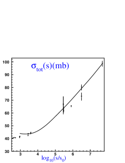
Figure 1: The GLM results compared to data for $\sigma_{tot}$.

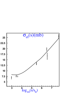
Figure 2: The GLM results compared to data for $\sigma_{el}$.

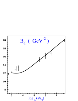
Figure 3: The GLM results compared to data for $B_{el}$.

W	$\sigma^{model}_{tot}$(mb)	$\sigma^{exp}_{tot}$(mb)	$\sigma^{model}_{el}$(mb)	$\sigma^{exp}_{el}$(mb)
7 TeV	98.6	TOTEM: 98.6 $\pm$2.2	24.6	TOTEM: 25.4$\pm 1.1$

W	$\sigma^{model}_{in}(mb)$	$\sigma^{exp}_{in}$(mb)	$B^{model}_{el}(GeV^{-2})$	$B^{exp}_{el}(GeV^{-2})$
7 TeV	74.0	CMS: 68.0$\pm 2^{syst}\pm 2.4^{lumi}\pm 4^{extrap}$	20.2	TOTEM: 19.9$\pm 0.3\,$
		ATLAS: 69.4$\pm 2.4^{exp}\pm 6.9^{extrap}$
		ALICE: 73.2 $(+2./-4.6)^{model}\pm 2.6^{lumi}$
		TOTEM: 73.5 $\pm 0.6^{stat}\pm 1.8^{syst}$

W	$\sigma^{model}_{sd}(mb)$	$\sigma^{exp}_{sd}$(mb)	$\sigma^{model}_{dd}$(mb)	$\sigma^{exp}_{dd}$(mb)
7 TeV	10.7GW + 4.18nGW	ALICE : 14.9(+3.4/-5.9)	6.21GW + 1.24nGW	ALICE: 9.0 $\pm$ 2.6

W	$\sigma^{model}_{tot}$(mb)	$\sigma^{exp}_{tot}$(mb)
57 TeV	130	AUGER: 133 $\pm 13^{stat}\pm 17^{sys}\pm 16^{Glauber}$
	$\sigma^{model}_{inel}$(mb)	$\sigma^{exp}_{inel}$(mb)
	95.2	AUGER: 92 $\pm 7^{stat}\pm 11^{syst}\pm 7^{Glauber}$

Table 1: .

Comparison of the values obtained from the GLM model with experimental results at W = 7 and 57 TeV.

.4 Alternative Models

There are several models on the market today that manage to reproduce the LHC experimental results. The most promising of these are summarized here, and their results are compared with those of GLM GLM1 in Table I.

The Durham group’s approach for describing soft hadron-hadron scattering RMK1 is similar to the GLM GLM1 approach, they include both enhanced and semi-enhanced diagrams. The two groups utilize different techniques for summing the multi-Pomeron diagrams. The Durham group have a bare (prior to screening) QCD Pomeron, with intercept $\Delta_{bare}$ = 0.32. This model RMK1 which was tuned to describe collider data, predicts values for $\sigma_{tot}$, $\sigma_{el}$ and $\sigma_{inel}$, which are lower than the TOTEM TOTEM data. To be consistent with the TOTEM results, RMK RMK2 have proposed an alternative formulation, based on a 3-channel eikonal description, with 3 diffractive eigenstates of different sizes, but with only one Pomeron whose intercept and slope are: $\Delta_{I\!\!P}$ = 0.14; $\alpha^{{}^{\prime}}_{I\!\!P}$ = 0.1 GeV^-2. Their results are shown in Table II in the column KMR2.

Ostapchenko OS [pre LHC] has made a comprehensive calculation in the framework of Reggeon Field Theory, based on the resummation of both enhanced and semi-enhanced Pomeron diagrams. To fit the total and diffractive cross sections he assumes two Pomerons: (for his solution set C) ”Soft Pomeron” $\,\,\,\alpha^{Soft}=1.14\,+\,0.14t$ and a ”Hard Pomeron” $\,\,\,\alpha^{Hard}=1.31\,+\,0.085t$. His results are quoted in Table II, in the column Ostap(C).

Kaidalov-Poghosyan KP have a model which is based on Reggeon calculus, they attempt to describe data on soft diffraction taking into account all possible non-enhanced absorptive corrections to 3 Reggeon vertices and loop diagrams. It is a single Pomeron model and with secondary Regge poles, their Pomeron has the following intercept and slope: $\Delta_{I\!\!P}\;=\;0.12$ and $\alpha^{{}^{\prime}}_{I\!\!P}\;=\;0.22$ GeV^-2. Their results are shown in Table II, in the column KP.

Ciesielski and Goulianos have proposed an ”event generator” BMR which is based on the BMR-enhanced PYTHIA8 simulation. In Table II their results are denoted by BMR.

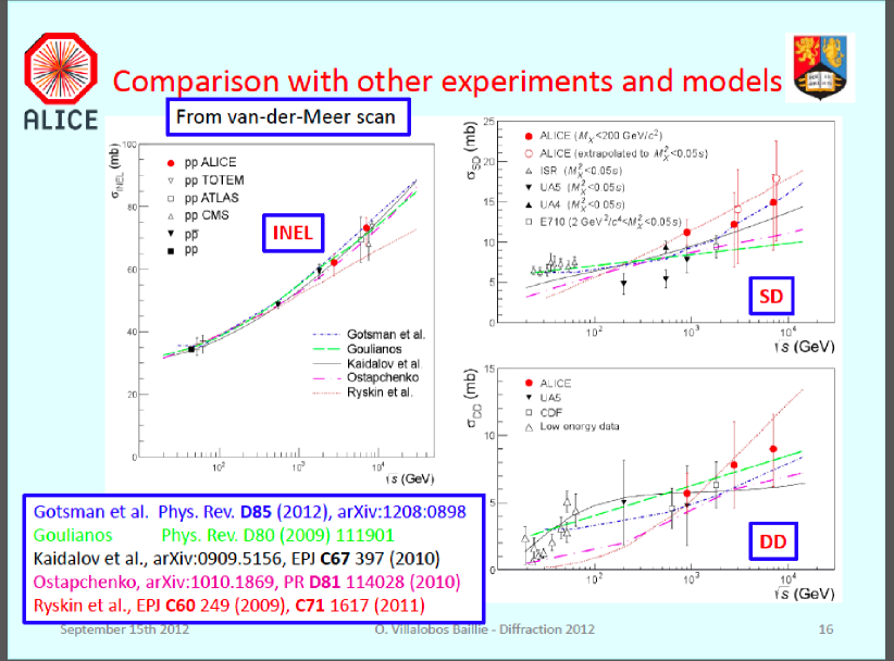
Figure 4: Comparison of Models with LHC data from Villalabos Ballie’s talk at Diffraction 2012. Villa4

W = 1.8 TeV	GLM	KMR2	Ostap(C)	BMR∗	KP
$\sigma_{\rm tot}(mb)$	79.2	79.3	73.0	81.03	75.0
$\sigma_{\rm el}(mb)$	18.5	17.9	16.8	19.97	16.5
$\sigma_{SD}(mb)$	11.27	5.9(LM)	9.2	10.22	10.1
$\sigma_{DD}(mb)$	5.51	0.7(LM)	5.2	7.67	5.8
$B_{el}(GeV^{-2})$	17.4	18.0	17.8

$W$ = 7 TeV	GLM	KMR2	Ostap(C)	BMR	KP
$\sigma_{\rm tot}$(mb)	98.6	97.4	93.3	98.3	96.4
$\sigma_{\rm el}$(mb)	24.6	23.8	23.6	27.2	24.8
$\sigma_{SD}$(mb)	14.88	7.3(LM)	10.3	10.91	12.9
$\sigma_{DD}$(mb)	7.45	0.9(LM)	6.5	8.82	6.1
$B_{el}$(GeV${}^{-2})$	20.2	20.3	19.0		19.0

$W$ = 14 TeV	GLM	KMR2	Ostap(C)	BMR	KP
$\sigma_{tot}$(mb)	109.0	107.5	105.	109.5	108.
$\sigma_{el}$(mb)	27.9	27.2	28.2	32.1	29.5
$\sigma_{SD}$(mb)	17.41	8.1(LM)	11.0	11.26	14.3
$\sigma_{DD}$(mb)	8.38	1.1(LM)	7.1	9.47	6.4
$B_{el}$(GeV${}^{-2})$	21.6	21.6	21.4		20.5

Table 2: Comparison of results of the different models for $W$ = 1.8, 7 and 14 TeV.

.5 Amplitudes

Until recently most of the comparison of models has been done on the level of cross-sections (which are areas), and only reveal the energy dependence, and therefore are not very helpful to discriminate between the different models. Having the behaviour of the various amplitudes as functions of impact parameter (momentum transfer) would be more revealing. Unfortunately, there is a paucity of material available on amplitudes, and most refer only to the elastic amplitude.

In Fig.5. we show elastic amplitudes emanating from the GLM model for various energies. We note the overall gaussian shape of the elastic amplitudes for all energies 0.545 $\leq\;W\;\leq$ 57 TeV, with the width and height of the gaussian growing with increasing energy. For small values of b the slope of the amplitudes decreases with increasing energy. The elastic amplitude (as $b\rightarrow$ 0) becomes almost flat for W = 57 TeV, where it is still below the Unitarity limit $A_{el}=1$ .

In Fig.6 we show the elastic, single diffraction and double diffraction amplitudes as functions of b for W = 7 TeV. Note the completely different shapes of the three amplitudes, the elastic amplitude $A_{el}(b)$ is gaussian in shape, while the single diffractive amplitude $A_{sd}(b)$ and the double diffractive amplitude $A_{dd}(b)$ are very small at small b . $A_{sd}$ has a peak at 1.25 fm, while $A_{dd}$’s maximum is at b = 2.15 fm.

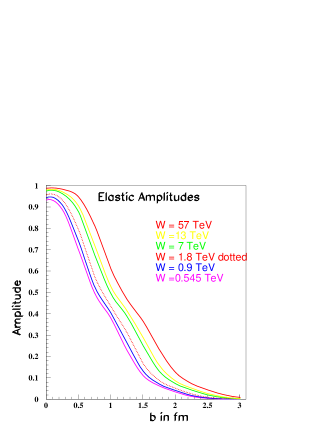
Figure 5: The GLM elastic amplitudes for LHC energies.

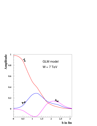
Figure 6: The GLM elastic, single diffractive and double diffractive amplitudes for W = 7 TeV.

The Durham group RMK2 have attempted to extract the form of the Elastic Opacity directly from the data.They assume that at high energies the real part of the scattering amplitude is very much smaller than the imaginary part, then to a good approximation

$$A(b)=i[1-\exp(-\Omega(b)/2)]$$

(see Eqn(1)). As $\Omega_{el}=-2ln(1-A_{el})$, they determine the Opacity directly from the data since

$${\rm Im}A(b)~{}=~{}\int\sqrt{\frac{d\sigma_{\rm el}}{dt}\frac{16\pi}{1+\rho^{2}}}~{}J_{0}(q_{t}b)~{}\frac{q_{t}dq_{t}}{4\pi},$$

where $q_{t}=\sqrt{|t|}$ and $\rho\equiv{\rm Re}A/{\rm Im}A$. Their results are shown in Fig. 7.

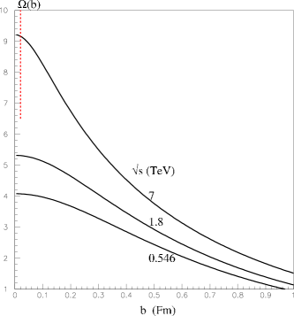
Figure 7: The proton opacity $\Omega(b)$ determined directly from the $pp$ $d\sigma_{\rm el}/dt$ data at 546 GeV , 1.8 TeV and 7 TeV data. The uncertainty on the LHC value at $b=0$ is indicated by a dashed red line. This figure is taken from RMK2

which should be consulted for details.

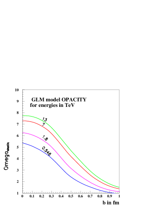
Figure 8: Opacites calculated using the GLM model.

The Durham group RMK2 find that at $Sp\bar{p}S$ and Tevatron energies the Opacity distributions have appoximately a Gaussian form. The analogous GLM model results are shown in Fig. 8, are in agreement with RMK2 regarding the shape of $\Omega_{el}(b)$, and in addition suggest that this is also true for the LHC energies. GLM find that with increasing energy, the intercept of the Opacity at b =0 increases, while the slope at small b decreases.

Ferreira, Kodama and Kohara FKK have recently made a detailed study of the proton-proton elastic amplitude for center of mass energy W = 7 TeV, based on Stochastic Vacuum Model (see FKK for more details).

In Fig.9 we show the GLM and FKK elastic amplitudes as a function of the impact parameter. Although the shapes are similar, the FKK amplitude is lower. If we normalize the FKK amplitude to the GLM value at b = 0, we note that the amplitudes which are gaussian in shape, have very similar behaviour as a function of the impact parameter.

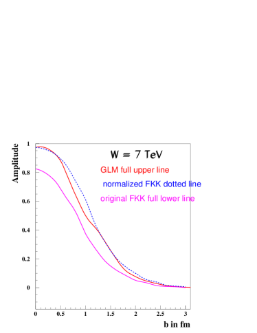
Figure 9: Comparison of the elastic amplitude determined by FKK FKK and the GLM model.

.6 Conclusions

We GLM1 have succeded in building a model for soft interactions, which provides a very good description all high energy data, including the LHC measurements. The model is based on a Pomeron with a large intercept ($\Delta_{I\!\!P}=0.23$) and very small slope ($\alpha^{\prime}_{I\!\!P}$ =0.028). We find no need to introduce two Pomerons: i.e. a soft and a hard one. The Pomeron in our model provides a natural matching with the hard Pomeron in processes that occur at short distances. The qualitative features of our model are close to what one expects from $N$=4 SYM GLM11 ; GLM12 , which is the only theory that is able to treat long distance physics on a solid theoretical basis.

In concluding I appeal to all model builders and Monte Carlo advocates to publish numerical values for their amplitudes, as this would enable one to check the inherent differences between the various approaches to soft scattering.

- (1) A. Donnachie, and P. V. Landshoff, Phys. Letters 296, 222 (1992).
- (2) A. Donnachie, and P. V. Landshoff, arXiv:1112.2485.
- (3) M. Froissart, Phys. Rev. 123, 1053 (1961). A. Martin, Nuovo Cimento 42A, 930 (1966) and arXiv:0812.0680v3.
- (4) E. Gotsman, E. Levin and U. Maor, Phys. Letters B716, 425 (2012), and references quoted there.
- (5) M. L. Good and W. D. Walker,Phys. Rev. 120, 1857 (1960).
- (6) E. Gotsman, E. Levin and U. Maor, Eur. Phys. J. C71, 1553 (2011).
- (7) E. Gotsman, E. Levin, U. Maor and J. S. Miller, Eur. Phys. J. C57, 689 (2008).
- (8) E. Gotsman, E. Levin and U. Maor, Phys. Rev. D 85, 094007 (2012).
- (9) O. Villalobos Baillie, talk at Diffraction 2012, Lanzarote, September 2012.
- (10) M. G. Poghosyan et al [ALICE Collaboration], J. Phys. G 38, 124044 (2011).
- (11) F. Ferro [TOTEM Collaboration], Europhys. Lett. 96, 21002 (2011).
- (12) G. Aad et al. [ATLAS Collaboration], Nature Commun. 2, 463 (2011).
- (13) S. Chatrchyan et al. [CMS Collaboration], arXiv:1210.6718 [hep-ex].
- (14) J. P. Revol, Proton-proton cross sections with multiplicities with ALICE at the LHC, talk at the Low-x Meetings, Phapos, Cyprus, June 27- July 1, 2012.
- (15) P. Abreu, et al. [Auger Collaboration], Phys. Rev. Letters 109, 062002 (20112).
- (16) M. G. Ryskin, A. D. Martin and V. A. Khoze, Eur. Phys. J. C71, 1617 (2011).
- (17) M. G. Ryskin, A. D. Martin and V. A. Khoze, Eur. Phys. J. C72, 1937 (2012).
- (18) S. Ostapchenko, Phys. Rev. D81, 114028 (2010).
- (19) A. B. Kaidalov and M. G. Poghosyan, arXiv:09095156 [hep-ph].
- (20) R. Ciesielski and K. Goulianos, arXiv:1205.1446.
- (21) E. Ferreira, T. Kodama and A.K. Kohara, Eur. Phys. J. C73, 2326 (2013).