Doubly Randomised Protocols for a Random Multiple Access Channel with “Success-Nonsuccess” Feedback

We consider a model of a decentralized multiple access system with a non-standard binary feedback where the empty and collision situations cannot be distinguished. We show that, like in the case of a ternary feedback, for any input rate $\lambda<e^{-1}$, there exists a “doubly randomized” adaptive transmission protocol which stabilizes the behavior of the system. We discuss also a number of related problems and formulate some hypotheses.

Keywords: random multiple access; binary feedback; positive recurrence; (in)stability; Foster criterion, fluid limit.

1 Introduction

We consider a decentralised multiple access system model with an infinite number of users, a single transmission channel, and an adaptive transmission protocol that does not use the individual history of messages. We consider a class of protocols where the user cannot observe the individual history of messages and the total number of messages. With any such a protocol, all users transmit their messages in time slot $(n,n+1)$ with equal probabilities $p_{n}$ that depend on the history of feedback from the transmission channel.

Algorithms with ternary feedback “Empty-Success-Collision” were introduced in [15] and [2]. It is assumed that the users can observe the channel output and distinguish among three possible situations: either no transmission (“Empty”) or transmission from a single server (“Success”) or a collision of messages from two or more users (“Conflict”). It is known since the 80’s (see e.g. [6], [10]) that if the feedback is ternary, then the channel capacity is $e^{-1}$: if the input rate is below $e^{-1}$, then there is a stable transmission protocol; and if the input rate is above $e^{-1}$, then any transmission protocol is unstable. A stable protocol may be constructed recursively as follows: given probability $p_{n}$ in time slot $(n,n+1)$ and a feedback at time $n+1$, probability $p_{n+1}$ is bigger than $p_{n}$ if the slot $(n,n+1)$ was empty, $p_{n+1}=p_{n}$ if there was a successful transmission, and $p_{n+1}$ is smaller than $p_{n}$ if there is a conflict. Hajek [6] considered a multiplicative increase/decrease and assumed that the random number, $\xi$, of arrivals per typical slot has a finite exponential moment, ${\mathbf{E}}e^{c\xi}<\infty$, for some $c>0$. Mihajlov [10] considered an additive increase/decrease and assume the second moment ${\mathbf{E}}\xi^{2}$ to be finite. Later Foss [5] showed that, without further assumptions on the input, condition $\lambda={\mathbf{E}}\xi<e^{-1}$ is sufficient for existence of an multiplicative stable algorithm, and extended this result onto a more general stationary ergodic input.

It is also known, see e.g. [8] and [11] that similar results (existence/nonexistence of a stable protocol if the input rate is below/above $e^{-1}$) hold for systems with either “Empty–Nonempty” binary feedback or “Conflict–Nonconflict” feedback.

In this paper we show that the channel capacity is again $e^{-1}$ for a third type of the binary feedback which may be called “Success–Nonsuccess” feedback. The problem is interesting from a practical point of view, because in order for a receiver to distinguish between “collision” and “no transmission”, it would have to differentiate between the increased energy or structure present when there is a collision of two or more packets, from thermal noise. That can be difficult or impossible for some receivers to do.

Tsybakov and Beloyarov, [13] and [14], introduced and studied a model with the “success-failure” feedback, but with an extra option. There is a selected in advance station which works as follows. Given a nonsuccess feedback, the station may send, in the next time slot, a testing package to recognize what has happened, either empty slot or collision. Clearly, if an algorithm uses this option regularly, it is an algorithm with the ternary feedback which works slower that the conventional one (uses two time slots instead of one in the case of nonsuccess). In [13] and [14], the authors introduce a class of algorithms that send a testing package from time to time only and show (numerically) that the lower is the rate of using this option, the closer to $e^{-1}$ is the throughput.

In this paper, we do not allow thus use of test packets. Our approach to the problem is to introduce a further (second) randomization. We consider a new class of “doubly randomised” protocols and show that, for any pair of numbers $0<\lambda_{0}<\lambda_{1}<e^{-1}$, there exists a protocol from the class that makes stable a system with input rate $\lambda$, for any $\lambda\in[\lambda_{0},\lambda_{1}]$. Then we formulate two conjectures on stability of other classes of protocols and, in particular of protocols that do not depend on an actual value of $\lambda$. Our stability result is based on a generalized Foster criterion and the fluid approximation approach, see e.g. [4].

In a recent paper [17] (see also [7]), a stability result has been obtained for a similar model with “success-failure” feedback where a user may also take into account the arrival time of its message. It was shown that if the input rate is below $0,317$, then there exist stable algorithms (called “algorithms with delayed intervals”). The results of our paper are stronger in two directions: we show that a stable protocol exists if the input rate is below $e^{-1}$ (clearly, $e^{-1}>0.317$) and that there is no need to use the information about arrival times.

There is an interesting question which seems to be open: assume we know arrival times of messages. Could this extra information increase an actual channel capacity?

The paper is organised as follows. Section 2 contains the description of the model and of the class of transmission protocols under consideration, as well as the statement of the main result. Its proof is presented in Section 3. Then in Section 4 we introduce two more classes of protocols and formulate conjectures on their stability.

2 The Model and the Class of Protocols

We consider (a variant of) a multi-access system introduced in [16]. There is an infinite number of users and a single transmission channel available to all of them. Users exchange their messages using the channel. Time is slotted and all message lengths are assumed to be equal to the slot length (and equal to one).

The input process of messages $\{\xi_{n}\}$ is assumed to be i.i.d., having a general distribution with finite mean $\lambda={\mathbf{E}}\xi_{1}$, here $\xi_{n}$ is a total number of messages arriving within time slot $[n,n+1)$ (we call it “time slot $n$”, for short).

The systems operates according to an “adaptive ALOHA protocol” that may be described as follows. There is no coordination between the users, and at the beginning of time slot $n$ each message present in the system is sent to the channel with probability $p_{n}$, independently of everything else. So given that the total number of messages is $N_{n}$, the number of those sent to the channel, $B_{n}$, has conditionally the Binomial distribution $B(N_{n},p_{n})$ (here $B_{n}\equiv 0$ if $N_{n}=0$). Let $J_{n}=1$ if $B_{n}=1$ and $J_{n}=0$, otherwise. If $J_{n}=1$, then there is a successful transmission within time slot $n$. Otherwise there is either an empty slot ($B_{n}=0$) or a collision of messages ($B_{n}\geq 2$), so there is no transmission. Then the following recursion holds:

$$N_{n+1}=N_{n}-J_{n}+\xi_{n+1}.$$ (1)

A transmission protocol is determined by sequence $\{p_{n}\}$. We consider “decentralised” protocols: the numbers $N_{n}$, $n=1,2,\ldots$ are not observable, and only values of past $J_{k},k<n$ are known. We consider protocols where $\{p_{n}\}$ are defined recursively in the Markovian fashion: $p_{n}$ is a (random) number that depends on the history of the system only through $p_{n-1}$ and $J_{n-1}$. Then a 2-dimensional sequence $(N_{n},p_{n}),\ n=1,2,\ldots$ forms a time-homogeneous Markov chain.

In the paper, we introduce three classes of decentralised protocols, prove a stability theorem for the first class and conjecture similar results for the two others. To describe these protocols, we introduce additional notation.

Let $N_{1}\geq 0$ be the initial number of messages in the system and $S_{1}\geq 1$ a positive number (which is an ”estimator” of unknown $N_{1}$). Let further $\beta\in(0,1),$ $C>0$ and $D>0$ be three positive parameters, and let $\{I_{n}\}$ be an i.i.d. sequence that does not depend on the previous r.v.’s, with ${\mathbf{P}}(I_{n}=1)=1-{\mathbf{P}}(I_{n}=0)=1/2$.

Remark 1.

In what follows, one can assume a sequence of estimators $\{S_{n}\}$ to take integer values only, by assuming that $D$ and $C$ are integer-valued. But this is not needed, in general.

The class ${\cal A}_{1}$ of algorithms is determined by $\beta$, $C>0$, $D>0$, $\{J_{n}\}$ and $\{I_{n}\}$ as follows. The transmission probabilities $p_{n}$ and the numbers $S_{n}$ are updated recursively: given $S_{n}$, we let

$$p_{n}=\begin{cases}\beta/S_{n}&\text{if}\ \ I_{n}=0,\\ 1/S_{n}&\text{if}\ \ I_{n}=1,\end{cases}$$

and then

$$S_{n+1}=\begin{cases}S_{n}+C&\text{if}\ \ J_{n}=0,\\ S_{n}+CD&\text{if}\ \ J_{n}=1\ \ \text{and}\ \ I_{n}=0,\\ \max(S_{n}-CD,1)&\text{if}\ \ J_{n}=1\ \ \text{and}\ \ I_{n}=1.\end{cases}$$

In words, the reason for second randomisation is as follows. When we get a successful transmission, we like keep our estimate $S_{n}$ not far from the right value of $N_{n}$ as long as possible. To increase our chances, we consider a randomised option for probability $p_{n}$, with taking two close, but not identical values, $\beta/S_{n}$ and $1/S_{n}$. So if we get success, we increase the $S$-value for the smaller probability and decrease for the bigger one.

We denote such an algorithm by $A_{1}(C,D,\beta)\in{\cal A}_{1}$. Two other classes of algorithms are defined in Section 4.

We can see that, with any algorithm introduced above, sequence $\{(N_{n},S_{n})\}$ forms a time-homogeneous Markov chain.

Definition 1. We say that a Markov chain $\{(N_{n},S_{n})\}$ is positive recurrent if there exists a compact set ${\cal K}\in{\cal R}_{+}^{2}$ such that

• for any pair of initial values $(N_{1},S_{1})=(N,S)$,

  $$\tau_{N,S}=\min\{n\geq 1\ :\ (N_{n},S_{n})\in{\cal K}\}<\infty\quad\mbox{a.s.}$$

• further,

  $$\sup_{(N,S)\in{\cal K}}{\mathbf{E}}\tau_{N,S}<\infty.$$

A Markov chain $\{(N_{n},S_{n})\}$ is Harris-ergodic if there is a probability distribution $\mu$ such that, for any initial value $(N_{1},S_{1})=(N,S)$, the distributions of $(N_{n},S_{n})$ converge to $\mu$ in the total variation,

$$\sup_{A}|{\mathbf{P}}((N_{n},S_{n})\in A)-\mu(A)|\to 0,\quad n\to\infty$$ (2)

where the supremum is taken over all Borel sets $A$ in ${\cal R}_{+}^{2}$.

It is well-known (see e.g. [9]) that a positive recurrent Markov chain $\{(N_{n},S_{n})\}$ is Harris-ergodic if it is aperiodic and there exist a positive integer $m$, a probability measure $\varphi$, and a positive number $c$ such that

$${\mathbf{P}}((N_{m},S_{m})\in\cdot\ |\ (N_{1},S_{n})=(N,S))\geq c\varphi(\cdot),$$ (3)

for all $(N,S)\in{\cal K}$.

Definition 2. We say that Markov chain $\{(N_{n},S_{n})\}$ is transient if there is an initial value $(N_{1},S_{1})=(N,S)$ such that $N_{n}+S_{n}\to\infty$ a.s., as $n\to\infty$.

Definition 3. Algorithm $A$ is stable if the underlying Markov chain $(N_{n},S_{n})$ determined by $A$ is Harris-ergodic, and unstable if the underlying Markov chain is transient.

Here is our main result.

Theorem 1.

Let $0<\lambda_{0}<\lambda_{1}<e^{-1}$ be any two numbers. There exist $C>0$, $\beta_{1}\in(0,1)$ such that, for any fixed $\beta\in(\beta_{1},1)$, there exists $D_{0}=D_{0}(\lambda_{0},\lambda_{1},\beta)$ such that, for any $D\geq D_{0}$, algorithm $A_{1}(C,D,\beta)$ is stable for any input rate $\lambda\in[\lambda_{0},\lambda_{1}].$

Remark 2.

If $\lambda>e^{-1}$, then any algorithm with a binary feedback is unstable, since the same result is known for any algorithm with a ternary feedback.

3 Proof of Theorem 1

We need to introduce a number of auxiliary functions: for positive numbers $\beta,\lambda,C,D$ and for $0\leq z<\infty$, let

$$j_{1}(z,\beta) = \frac{\beta z}{2}e^{-\beta z},\ \ j_{2}(z)=\frac{z}{2}e^{-z};$$ (4)

$$j(z,\beta) = j_{1}(z,\beta)+j_{2}(z);$$ (5)

$$a(z,\beta) = \lambda-j(z,\beta);$$ (6)

$$b(z,\beta) = C(1-j(z,\beta))+CD(j_{1}(z,\beta)-j_{2}(z));$$ (7)

$$r(z,\beta) = a(z,\beta)-zb(z,\beta).$$ (8)

Cleary, for any $\beta>0$ and as $z\to\infty$, $j_{1}(z,\beta),j_{2}(z)$ and $j(z,\beta)$ tend to 0, $a(z,\beta)\to\lambda$, $b(z,\beta)\to C$, and $r(z,\beta)\to-\infty$.

We rely on the following auxiliary result.

Lemma 1.

The functions $j(z,\beta),a(z,\beta),b(z,\beta)$ and $r(z,\beta)$ satisfy the following conditions:
for any $0<\lambda_{0}<\lambda_{1}<e^{-1}$, there exists $\beta_{1}\in(0,1)$ such that, for any $\lambda\in[\lambda_{0},\lambda_{1}]$, $\beta\in(\beta_{1},1)$ and for any $C\geq C_{1}:=\frac{\lambda_{1}+1}{1-e^{-1}}$ and $D\geq D(C)$ (where $D(C)$ is specified in the proof, see equality (12) below),

• equation $a(z,\beta)=0$ has two roots $0<z_{1}<z_{2}<\infty$;

• equation $b(z,\beta)=0$ has two roots $0<t_{1}<t_{2}<\infty$;

• $0<t_{1}<z_{1}<t_{2}<z_{2}$;

• function $r$ is continuous in $z\in[0,\infty]$, $r(z,\beta)>0$ for $z\leq z_{1}$ and $r(z,\beta)<0$ for $z\geq t_{2}$; therefore $\inf_{0\leq z\leq z_{1}}r(z,\beta)>0$, $\sup_{t_{2}\leq z\leq\infty}r(z,\beta)<0$ and all roots to equation $r(z,\beta)=0$ lie in the interval $(z_{1},t_{2})$.

Proof. Introduce a further function

$$b_{1}(z,\beta)=1-j(z,\beta)+D(j_{1}(z,\beta)-j_{2}(z)).$$

Then $b(z,\beta)=Cb_{1}(z,\beta)$.

We know that $ze^{-z}$ (and also $j_{2}(z)$) is increasing in $z$ if $z\in(0,1)$ and decreasing if $z>1$. Then, for $\beta<1$, $j_{1}(z,\beta)$ is increasing if $z<1/\beta$ and decreasing if $z>1/\beta$. Further, $m(\beta):=\min_{1\leq z\leq 1/\beta}j(z,\beta)$ is strictly positive and tends to $e^{-1}$ as $\beta\uparrow 1$.

For any $\lambda_{1}\in(0,e^{-1})$ and any $\varepsilon\in(0,e^{-1}-\lambda_{1})$, one can choose $\widehat{\beta}_{1}<1$ so close to 1 that $m(\beta)\geq\lambda_{1}+\varepsilon$, for all $\beta\in[\widehat{\beta}_{1},1)$. Then for any $\lambda\in(0,\lambda_{1}]$ and any $\beta\in[\widehat{\beta}_{1},1]$, equation $j(z,\beta)=\lambda$ has two roots, $z_{1}(\beta,\lambda)$ and $z_{2}(\beta,\lambda)$, with

$$z_{1}(\beta,\lambda)\leq z_{1}(\beta,\lambda_{1})<1<z_{2}(\beta,\lambda_{1})\leq z_{2}(\beta,\lambda).$$

By continuity of functions under consideration, for any $\lambda\leq\lambda_{1}$, $\beta z_{2}(\beta,\lambda)\to z_{2}(1,\lambda)$ as $\beta\uparrow 1$, so one can choose $\beta_{1}\in[\widehat{\beta}_{1},1)$ such that

$$\inf_{\lambda\in(0,\lambda_{1}]}\inf_{\beta\in[\beta_{1},1]}\beta z_{2}(\beta,\lambda)>1.$$

Then, again for all $\lambda\in(0,\lambda_{1}]$ and all $\beta\in[\beta_{1},1)$,

$$j_{1}(z_{1},\beta)-j_{2}(z_{1})<0<j_{1}(z_{2},\beta)-j_{2}(z_{2}),$$ (9)

with $z_{i}=z_{i}(\beta,\lambda)$, for $i=1,2$.

Now we fix $\beta\in[\beta_{1},1)$ and, for given $0<\lambda_{0}<\lambda_{1}$, let

$$D_{0}=\frac{2}{\inf_{\lambda_{0}\leq\lambda\leq\lambda_{1}}(j_{2}(z_{1})-j_{1}(z_{1},\beta))}<\infty.$$ (10)

Then, for any $D\geq D_{0}$ and for any $\lambda\in[\lambda_{0},\lambda_{1}]$, we have $b_{1}(z_{1},\beta)<0$ and $b_{1}(z_{2},\beta)>0$ (the latter inequality always holds).

Take any $D\geq D_{0}$ and let $t_{1}<t_{2}$ be the roots to equation $b_{1}(z,\beta)=0$ (one can easily show that the latter equation has exactly two roots). Then, clearly, $0<t_{1}<z_{1}<t_{2}<z_{2}$.

Further, we may choose $C$ such that all roots of equation $r(z)=0$ lie in the interval $(z_{1},t_{2})$. Indeed, for $z>z_{2}\geq 1$ and $\lambda\leq\lambda_{1}$,

$$r(z,\beta) = \lambda-j(z,\beta)-Cz(1-j(z,\beta))-CDz(j_{1}(z,\beta)-j_{2}(z))$$

$$\leq \lambda_{1}-C(1-e^{-1})\leq-1$$

if

$$C\geq C_{1}:=\frac{\lambda_{1}+1}{1-e^{-1}}.$$ (11)

Further, for $z\leq t_{1}\leq 1$ and $\lambda\geq\lambda_{0}$,

$$r(z,\beta) > \lambda-j(z,\beta)-Cz(1-j(z,\beta))$$

$$\geq \lambda-j(t_{1},\beta)-Ct_{1}$$

$$\geq \lambda_{0}-(1+C)t_{1}$$

since $j(t_{1},\beta)\leq t_{1}e^{-t_{1}}\leq t_{1}$. The value of $t_{1}$ is decreasing to $0$ as $D$ tends to infinity. Therefore, one can choose $D_{1}=D_{1}(C)$ such that $(1+C)t_{1}\leq\lambda_{0}/2$ for any $D\geq D_{1}$, and then let

$$D(C)=\max(D_{0},D_{1}).$$ (12)

In more detail, since $\sup_{t_{0}\leq t\leq 1}\frac{1-j(t,\beta)}{j_{2}(t)-j_{1}(t,\beta)}<\infty$ for any $0<t_{0}<1$ and since $\lim_{t\downarrow 0}\frac{1-j(t,\beta)}{j_{2}(t)-j_{1}(t,\beta)}=\infty,$ we may choose $D_{1}=D_{1}(C)$ so large that

$$t(D_{1})=\max\{t\in(0,1)\ :\ \frac{1-j(t,\beta)}{j_{2}(t)-j_{1}(t,\beta)}\geq D_{1}\}$$

satisfies inequality $t(D_{1})\leq\frac{\lambda_{0}}{2(C+1)}.$ Therefore, for any $D\geq D_{1}$, we have $t_{1}<t(D_{1})\leq\frac{\lambda_{0}}{2(C+1)}.$

It is left to comment that $r(z,\beta)>0$ for $z\in(t_{1},z_{1}]$ since $a(z,\beta)\geq 0$ and $b(z,\beta)<0$, and that $r(z,\beta)<0$ for $z\in[t_{2},z_{2})$ since $a(z,\beta)<0$ and $b(z,\beta)\geq 0$.

The proof of the lemma is complete.

Now we apply the lemma to the proof of the theorem as follows.

We fix $\beta$ and write $j(z)$, $a(z)$, $b(z)$ and $r(z)$ instead of $j(z,\beta)$, $a(z,\beta)$, $b(z,\beta)$ and $r(z,\beta)$, for short.

Step 1. We introduce fluid limits for the Markov chain under consideration. Let Markov Chain $(N_{k}^{m_{0}},S_{k}^{s_{0}})$ start from initial values $N_{0}=m,S_{0}=s$ and assume that $v:=m+s\to\infty$ and that $m/v\to x,s/v\to y$ where $x+y=1$ and $x,y\geq 0$. Consider a continuous-time Markov process $(N^{m}(t),S^{s}(t))$ where

$$N^{m}(t)=N_{[tv]}^{m},\ S^{s}(t)=S_{[tv]}^{s}$$

and $[z]$ is the integer part of number $z$. Then we consider a family of weak limits of these processes, as $v\to\infty$. They are indexed by their initial value $(x_{0},y_{0})$ with $x_{0}\geq 0$, $y_{0}\geq 0$, $x_{0}+y_{0}=1$. By following the standard scheme (see, e.g., [12], [3], [1]), one can easily show that each such a limit, say $(\widetilde{N}(t),\widetilde{S}(t))$ is a Lipschitz function with continuous derivatives, and its derivatives are the functions $a(z)$ and $b(z)$ that were introduced earlier. In more detail, for any $x_{0},y_{0}\geq 0,x_{0}+y_{0}=1$, for any fluid limit $(\widetilde{N}(t),\widetilde{S}(t)),t\geq 0$ that starts from initial value $\widetilde{N}(0)=x_{0},\widetilde{S}(0)=y_{0}$, and for any time $t\geq 0$, if $\widetilde{N}(t)+\widetilde{S}(t)>0$, we let $z=z(t)=\widetilde{N}(t)/\widetilde{S}(t)\in[0,\infty]$. Then the derivatives are $d\widetilde{N}(t)/dt=a(z)$ and $d\widetilde{S}(t)/dt=b(z).$

To see that the derivatives are $a(z)$ and $b(z)$ indeed, we may find the one-step drift. We have

$$j(m,s):={\mathbf{E}}(J_{n}\ |\ N_{n}=m,S_{n}=s)=\frac{m\beta}{2s}\left(1-\frac{\beta}{s}\right)^{m-1}+\frac{m}{2s}\left(1-\frac{1}{s}\right)^{m-1}.$$

Then

$$a(m,s):={\mathbf{E}}(N_{n+1}-N_{n}\ |\ N_{n}=m,S_{n}=s)=\lambda-j(m,s).$$

In the conditions of Theorem 1, and for $s>CD$,

$$b(m,s):={\mathbf{E}}(S_{n+1}-S_{n}\ |\ N_{n}=m,S_{n}=s)=C(1-j(m,s))+CD\left(\frac{m\beta}{2s}\left(1-\frac{\beta}{s}\right)^{m-1}-\frac{m}{2s}\left(1-\frac{1}{s}\right)^{m-1}\right).$$

Then, as $m+s\to\infty$, $m/s\to z$,

$$j(m,s)\to j(z),\ \ \ a(m,s)\to a(z),\ \ \ b(m,s)\to b(z).$$

Step 2. We have to show next that any fluid limit $(\widetilde{N}(t),\widetilde{S}(t))$ (that starts from initial value $(\widetilde{N}(0),\widetilde{S}(0))$ with $\widetilde{N}(0)+\widetilde{S}(0)=1$) is stable in the following sense: for some $\varepsilon\in(0,1)$, there exists finite time $t_{\varepsilon}$ such that $\widetilde{N}(t_{\varepsilon})+\widetilde{S}(t_{\varepsilon})\leq 1-\varepsilon$. Then, by the general theory (see e.g. [1]), the positive recurrence of the underlying Markov chains follows.

In the positive quadrant ${\cal R}^{2}\setminus\{(0,0)\}=\{(x,y)\ :\ x,y\geq 0,x+y>0\}$, introduce a vector field of “rates”: the rate from point $(x,y)$ is $(a(z),b(z))$ where $z=x/y$. From the lemma and Step 1, we may deduce that this vector field is “self-similar” (rates do not change along any line with tangent $z$ that starts from the origin). Functions $(a(z),b(z))$ are continuous in $z\in[0,\infty]$. Since $a(0)>0,b(0)>0,a(\infty)>0,b(\infty)>0$ and the functions change their signs in the “right” order $0<t_{1}<z_{1}<t_{2}<z_{2}$, we have, in particular, $a(z)<0,b(z)<0$ for $z\in(z_{1},t_{2})$ and $\inf_{z}(|a(z)|+|b(z)|)>0$. Each trajectory of a fluid limit (fluid trajectory, for short) is a “geodesic” line with respect to this vector field.

From the properties of function $r$ in Lemma 1, it follows that any fluid trajectory moves towards the cone ${\cal C}:=\{(x,y)\ :\ x/y\in[z_{1},t_{2}]\}$, hits the cone at some time instant and then never leaves it and drifts towards the origin. To make this observation more rigorous, we introduce a positive function $R(z)$ with the following properties: $R(0)=1$ and the pair $(arctan(z),R(z))$, $0\leq z\leq\infty$ represents a graph (in the polar coordinates) of a smooth function that splits the positive quadrant into two domains (where one of the domains is a convex compact neighbourhood of the origin).

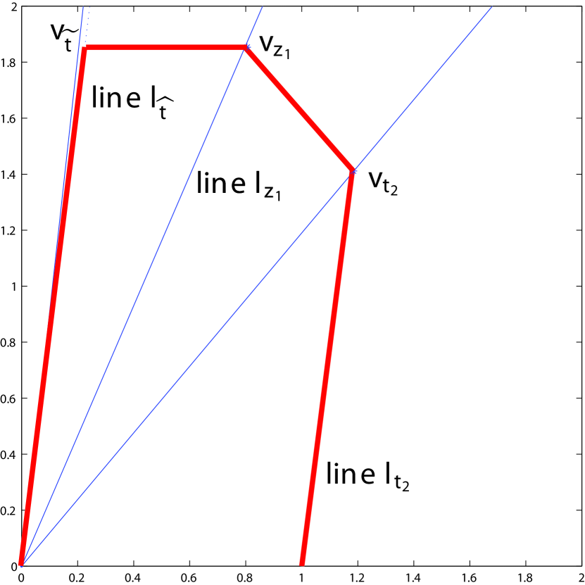
Figure 1: Graph L(x,y)=1 in case $\lambda=0.1$ $\beta=0.98$ $C=2.1$ $D=10000$

Then, for any constant $c>0$, we draw a line $(arctan(z),cR(z))$, and introduce a test function $L(x,y)$ by letting $L(x,y)=c$ if the point $(x,y)$ belongs the line $(arctan(z),cR(z))$. Further, the line is such that, for $c$ large enough, vector $(a(z),b(z))$ is directed into the compact domain, and its normal component to the line is not smaller than a certain positive value.

The construction follows a number of routine steps, therefore we provide a sketch of the proof and a clarifying figure only. First we construct a continuous piecewise-linear function. Then we make it smooth around the points where the line changes it direction.

We introduce the piecewise linear function as follows. We start from a fixed point, say $(1,0)$, on the abscissa. Since $\lambda/C<1<t_{2}$, we may choose an angle slightly bigger than $arctan(\lambda/C)$, say $\varphi\in(arctan(\lambda/C),\pi/4)$, and draw a straight line from $(1,0)$ under angle $\varphi$ (measured from the ordinate line). It intersects the line $l_{t_{2}}$ with tangent $t_{2}$ that starts from the origin (again we measure the tangent with respect to the ordinate line) at some point, say $v_{t_{2}}$. From this point, we draw another straight line at the angle $-\pi/4$ until it crosses the line $l_{z_{1}}$ with tangent $z_{1}$ (that starts from the origin) at some point, say $v_{z_{1}}$.

Now we recall that $\lambda/C>t_{1}$, see the proof of the lemma. Therefore one can take any $\varepsilon\in(0,(\lambda/C-t_{1})/2)$, let $\widehat{t}=t_{1}+\varepsilon$ and draw a line $l_{\widehat{t}}$ with tangent $\widehat{t}$ from the ordinate line that starts from the origin. Starting from point $v_{z_{1}}$, we draw a horizontal line in the left direction, and it intersects with $l_{\widehat{t}}$ at some point, say $v_{\widehat{t}}$. Finally, starting from $v_{\widehat{t}}$, we draw a straight line under the angle $arctan(\lambda/C-\varepsilon)$ in the left-down direction until it crosses the ordinate line, say at point $v_{0}$.

Therefore, we have drawn a continuous and convex piece-wise linear line. Then we make it smooth (say differentiable) by changing in small neighbourhoods of the corners (around points $v_{t_{2}},v_{z_{1}}$ and $v_{\widehat{t}}$), with keeping it convex. This completes the construction of the line $L(x,y)=1$.

Recall that all other lines $L(x,y)=c$ are obtained by the scaling. Then, using routine calculations and the properties of function $r$, one can show that, for $c$ large enough and for each $z\in[0,\infty]$, the drift vector $(a(z),b(z))$ is directed into the compact domain $\{(x,y)\ :\ L(x,y)\leq c\}$, and its normal projection is uniformly positive for all $z\in[0,\infty]$. This implies positive recurrence of the underlying Markov chain.

To conclude that Harris conditions hold we observe that the compact domain contains only a finite of states (since $N_{n}$ and $S_{n}$ are integer-valued), that all these states intercommunicate, and that the Markov chain is aperiodic since ${\mathbf{P}}(\xi_{1}=0)>0$. This completes the proof of the theorem.

4 Conjectures

Here we introduce two more classes of transmission protocols and conjecture corresponding stability results.

Let ${\cal H}$ be a class of functions $h:[1,\infty)\to[0,\infty)$ such that $h(1)=0$, $h(x)\uparrow\infty$ is non-decreasing in $x$, $x-h(x)\uparrow\infty$ is non-decreasing in $x$, and $h(x)/x\to 0$, as $x\to\infty$. With each $h\in{\cal H}$, we associate a class ${\cal E}_{h}$ of positive functions $\varepsilon_{h}:[1,\infty)\to(0,1/2]$, such that $\varepsilon_{h}(x)\to 0$ and $h(x)\varepsilon^{2}(x)\to\infty$, as $x\to\infty$.

The two other classes of algorithms differ from the first class in the following.

Algorithms from the second class ${\cal A}_{2}$ differ from those from the class ${\cal A}_{1}$ only in a way the $S$’s are updated: the constant $CD$ is replaced by a function $h\in{\cal H}$. More precisely, the algorithms are determined by $\beta$, $C$, $h(x)$, $\{J_{n}\}$ and $\{I_{n}\}$. Given $S_{n}$, we again let

$$p_{n}=\begin{cases}\beta/S_{n}&\text{if}\ \ I_{n}=0,\\ 1/S_{n}&\text{if}\ \ I_{n}=1,\end{cases}$$

but now define $S_{n+1}$ by

$$S_{n+1}=\begin{cases}S_{n}+C&\text{if}\ \ J_{n}=0,\\ S_{n}+h(S_{n})&\text{if}\ \ J_{n}=1\ \ \text{and}\ \ I_{n}=0,\\ \max(S_{n}-h(S_{n}),1)&\text{if}\ \ J_{n}=1\ \ \text{and}\ \ I_{n}=1.\end{cases}$$

For this algorithm, we use notation $A_{2}(C,h,\beta)\in{\cal A}_{2}$.

We modify further the class 2 algorithms by replacing $\beta$ by $1-\varepsilon_{h}$, this will form the third class ${\cal A}_{3}$. More precisely, the algorithms are determined by $C$, $h$, $\varepsilon_{h}$, $\{J_{n}\}$ and $\{I_{n}\}$. Given $S_{n}$, we now let

$$p_{n}=\begin{cases}(1-\varepsilon_{h}(S_{n}))/S_{n}&\text{if}\ \ I_{n}=0,\\ 1/S_{n}&\text{if}\ \ I_{n}=1,\end{cases}$$

and then define $S_{n+1}$ as for class 2 algorithms:

$$S_{n+1}=\begin{cases}S_{n}+C&\text{if}\ \ J_{n}=0,\\ S_{n}+h_{(}S_{n})&\text{if}\ \ J_{n}=1\ \ \text{and}\ \ I_{n}=0,\\ \max(S_{n}-h(S_{n}),1)&\text{if}\ \ J_{n}=1\ \ \text{and}\ \ I_{n}=1.\end{cases}$$

For this algorithm, we use notation $A_{3}(C,h,1-\varepsilon_{h})\in{\cal A}_{3}$.

We can see that again, with any algorithm from the classes ${\cal A}_{2}$ or ${\cal A}_{3}$, a sequence $\{(N_{n},S_{n})\}$ forms a time-homogeneous Markov chain.

We believe that the following two statement should be true.

Conjecture 1. Let $0<\lambda_{0}<e^{-1}$ be any number. There exists $C>0$ and $\beta_{2}\in(0,1)$ such that, with any $\beta\in(\beta_{2},1)$ and any function $h\in{\cal H}$, algorithm $A_{2}(C,h,\beta)$ stabilizes the system, for any input rate $\lambda<\lambda_{0}$.
If, on the contrary, either $\beta<\beta_{2}$ or $\lambda>\lambda_{0}$ , then the algorithm $A_{2}(C,h,\beta)$ is unstable in the system with input rate $\lambda$, for any $h\in{\cal H}$.

Conjecture 2. Any algorithm $A_{3}(C,h,1-\varepsilon_{h})$ from the third class stabilizes the system, for any input rate $\lambda<e^{-1}$.

Remark 3.

The conjectures may hold for a broader classes of algorithms if one assumes that, in the recursion for $S_{n}$, function $h$ is replaced by two functions, $h_{1}$ in the second line and $h_{2}$ in the third line.

References

- [1] M. Bramson. Stability of queueing networks Lecture Notes in Mathematics, 1950. Berlin: Springer, 2008.
- [2] J. L. Capetanakis. Tree algorithms for packet broadcast channels. IEEE Transactions on Information Theory, 25(5): 505–515, 1979.
- [3] J. G. Dai. On positive Harris recurrence of multiclass queueing networks: a unified approach via fluid limit models. Annals of Applied Probability, 5: 49–77, 1995.
- [4] S. Foss, T. Konstantopoulos. An overview of some stochastic stability methods. Journal of Operation Research Society Japan, 47(4):275–303, 2004.
- [5] S. Foss. Stochastic Recursive Sequences and Their Applications in Queueing Theory. Dissertation for the Degree of Doctor of Sciences, June 1992, Institute of Mathematics, Novosibirsk.
- [6] B. Hajek and T. van Loon. Decentralized dynamic control of a multiaccess broadcast channel. IEEE Trans. Automatic Control, 27(3): 559 - 569, 1982.
- [7] A. Malkov, A. Turlikov. Random multiple access protocols for communication systems with ”success-failure” feedback. IEEE International Workshop on Information Theory, 1–39, 1995.
- [8] N. Mehravari, T. Berger. Poisson multiple-access contention with binary feedback. IEEE Transactions on Information Theory, 30(5): 745–751, 1984.
- [9] S. Meyn and R.L. Tweedie. Markov Chains: Stochastic Stability. Springer, 1993.
- [10] V.A. Mihajlov. Geometrical Analysis of the Stability of Markov Chains in and Its Application to Throughput Evaluation of the Adaptive Random Multiple Access Algorithm. Problems of Information Transmission, 24(1): 47–56, 1988.
- [11] B. Paris, B. Aazhang. Near-optimum control of multiple-access collision channels. IEEE Transactions on Wireless Communications, 40: 1298–1308, 1992.
- [12] A. Rybko, A. Stolyar. Ergodicity of stochastic processes describing the operations of open queueing networks. Problems of Information Transmission, 28(1): 199-220, 1992.
- [13] B.S. Tsybakov, A.N. Beloyarov. Random multiple access in a channel with a binary feedback “Success-Failure”. Problems of Information Transmission, 26(3): 67–82, 1990.
- [14] B.S. Tsybakov, A.N. Beloyarov. Random multiple access in a channel with a binary feedback. Problems of Information Transmission, 26(4): 83–97, 1990.
- [15] B.S. Tsybakov, V.A. Mihajlov. Free synchronized access in a broadcast channel with a feedback. Problems of Information Transmission, 14(4): 32–59, 1978.
- [16] B.S. Tsybakov, V.A. Mihajlov. Random multicle access of packets. Splitting algorithm. Problems of Information Transmission, 16(4): 65–79, 1980.
- [17] A. Turlikov and S. Foss. On ergodic algorithms in random multiple access systems with “success-failure” feedback. Problems of Information Transmission, 46(2): 185–201, 2010.