Uniform generation of RNA pseudoknot structures with genus filtration

Abstract

In this paper we present a sampling framework for RNA structures of fixed topological genus. We introduce a novel, linear time, uniform sampling algorithm for RNA structures of fixed topological genus $g$, for arbitrary $g>0$. Furthermore we develop a linear time sampling algorithm for RNA structures of fixed topological genus $g$ that are weighted by a simplified, loop-based energy functional. For this process the partition function of the energy functional has to be computed once, which has $O(n^{2})$ time complexity.

1 Introduction

Pseudoknots have long been known as important structural elements in RNA [1]. These cross-serial interactions between RNA nucleotides are functionally important in tRNAs, RNaseP [2], telomerase RNA [3], and ribosomal RNAs [4]. Pseudoknots in plant virus RNAs mimic tRNA structures, and in vitro selection experiments have produced pseudoknotted RNA families that bind to the HIV-1 reverse transcriptase [5]. Import general mechanisms, such as ribosomal frame shifting, are dependent upon pseudoknots [6].

Lyngsø et al. [7] have shown that the prediction of general RNA pseudoknot structures is NP-complete. Thus, in order to provide prediction tools of feasible time complexity one frequently sticks to subtle subclasses of pseudoknots suitable for the dynamic programming paradigm [8, 9]. Alternative approaches to the prediction of RNA secondary structure (with or without pseudoknots) build on random sampling of foldings compatible to a given sequence. Here both, the underlying probability model and the efficiency of the sampling algorithm are crucial for being successful.

In this paper we propose a linear time uniform random sampler for pseudoknotted RNA structures of given genus which might be considered a promising starting point for the design of efficient solutions to the structure prediction problem. Our approach is based on the observation that pseudoknotted RNAs are in a natural way related to topological surfaces. In fact pseudoknotted RNA structures can be viewed as drawings on orientable surfaces of genus $g$, that is by means of the classical classification theorem either on the sphere (secondary structures) or connected sums of tori (pseudoknotted structures). Our approach is a natural evolution from Waterman et al. pioneering work [10, 11, 12] on secondary structures.

Secondary structures are coarse grained RNA contact structures, see Figure 1 (A). They can be represented as diagrams, i.e. labeled graphs over the vertex set $[n]=\{1,\dots,n\}$ with vertex degrees $\leq 3$, represented by drawing its vertices on a horizontal line and its arcs $(i,j)$ ($i<j$), in the upper half-plane, see Figure 1. We assume the vertices to be connected by the edges $\{i,i+1\}$, $1\leq i<n$, which are not considered arcs (but contribute to a nodes’s degree). Furthermore, vertices and arcs correspond to the nucleotides A, G, U and C and Watson-Crick base pairs (A-U, G-C) or wobble base pairs (U-G), respectively.

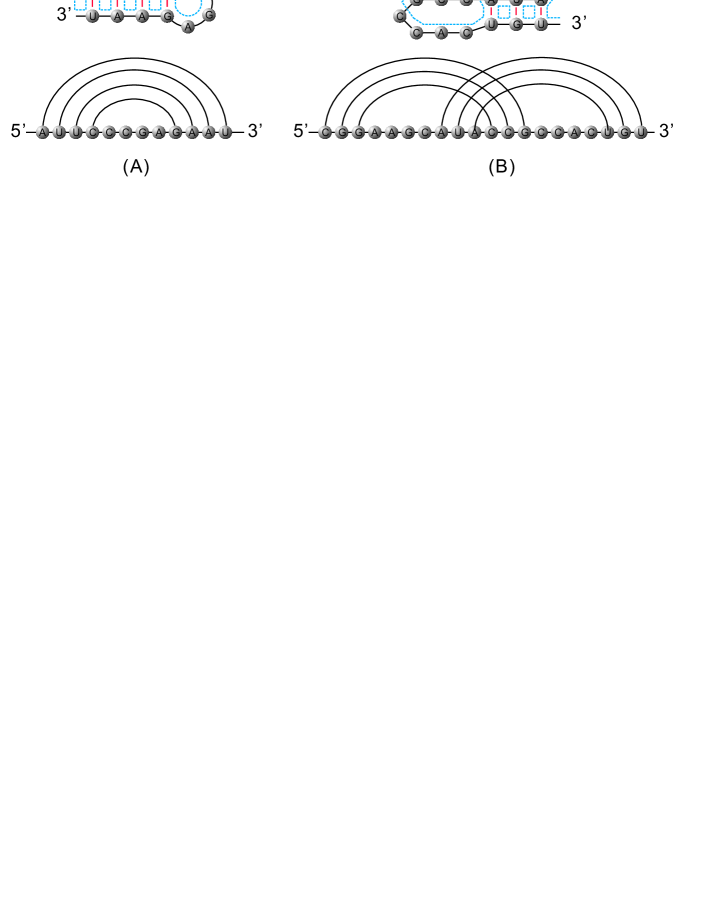
Figure 1: A secondary structure (A) and a pseudoknot structure (B) and their diagram representation.

Considering only the Watson-Crick and wobble base pair RNA structures, we set the restriction that one vertex can only paired with at most another vertex. Let $i<r$, we call arcs $(i,j)$ and $(r,s)$ crossing if $i<r<j<s$ holds. In this representation a secondary structure is a diagram without crossing arcs. Otherwise, i.e. diagrams with crossings represent pseudoknot structures, see Figure 1 (B).

In this paper, we present a framework for generating diagrams with crossings, filtered by topological genus, with uniform probabilities. The topological filtration of RNA structures has first been proposed by Penner and Waterman in [13] and later, as an application of the Matrix model [14], in [15]. The work here however is based on the combinatorial work of Chapuy [16].

In order to understand how topology enters the picture for RNA molecules we need to pass from diagrams or contact-graphs to that of topological surfaces. Only the associated surface carries the key invariants leading to a meaningful filtration of RNA structures. The mental picture here is to “thicken” the edges into (untwisted) bands and to expand each vertex to a disk as shown in Figure 2. This inflation of edges leads to a fatgraph $\mathbb{D}$ [17, 18].

A fatgraph, sometimes also called also a “map”, is a graph equipped with a cyclic ordering of the incident half-edges at each vertex. Thus, $\mathbb{D}$ refines its underlying graph $D$ insofar as it encodes the ordering of the ribbons incident on its disks. In fact a fatgraph constitutes to a cell-complex structure –combinatorial data in a sense– that have a topological surface as geometric realization [19].

Our sampling process consists of two steps: first we generate a diagram without crossing arcs and second we lift the topological genus to some fixed $g$. The process has linear time and is thereby very efficient.

The paper is organized as follows: we first introduce the topological filtration of diagrams. Then we introduce a genus induction process and finally, we describe and analyze the sampling processes.

2 Some basic facts

2.1 Diagrams

A diagram is a labeled graph over the vertex set $[n]=\{1,\dots,n\}$ in which each vertex has degree $\leq 3$, represented by drawing its vertices in a horizontal line. The backbone of a diagram is the sequence of consecutive integers $(1,\dots,n)$ together with the edges $\{\{i,i+1\}\mid 1\leq i\leq n-1\}$. The arcs of a diagram, $(i,j)$, where $i<j$, are drawn in the upper half-plane. We shall distinguish backbone edges $\{i,i+1\}$ from arcs $(i,i+1)$, which we refer to as a $1$-arc. Two arcs $(i,j)$, $(r,s)$, where $i<r$ are crossing if $i<r<j<s$ holds. The arc $(1,n)$ is called rainbow, see Figure 3.

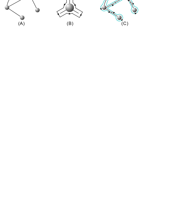
Figure 2: From graphs to fatgraphs: (A) A graph with $4$ vertexes and $4$ edges. (B) Inflation of a vertex. (C) A fatgraph derived from (A) induces a topological surface.

2.2 Fatgraphs and unicellular maps

In this section, we discuss the filtration of diagrams by topological genus. In order to extract topological properties of diagrams those need to be enriched to fatgraphs. The latter are tantamount to a cell-complex structures over topological surfaces. Formally, we make this transition [20] by “thickening” the edges of the diagram into (untwisted) bands or ribbons. Furthermore each vertex is inflated into a disc as shown in Figure 2 (B). This inflation of edges and vertices means to replace a set of incident edges by a sequence of half-edges. This constitutes the fatgraph $\mathbb{D}$ [17, 18].

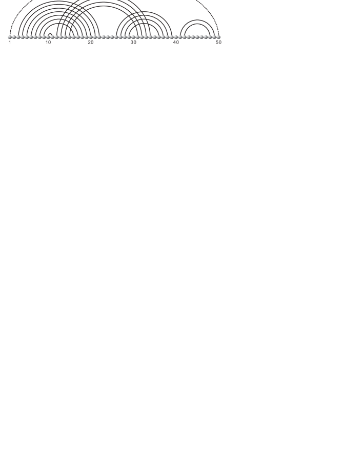
Figure 3: A diagram over $50$ vertices. The arc $(10,11)$ is a $1$-arc. The arcs $(3,22)$ and $(12,34)$ are crossing. The dashed arc $(1,50)$ is the rainbow.

A fatgraph is thus a graph enriched by a cyclic ordering of the incident half-edges at each vertex and consists of the following data: a set of half-edges, $H$, cycles of half-edges as vertices and pairs of half-edges as edges. Consequently, we have the following definition:

Definition 1.

A fatgraph is a triple $(H,\sigma,\alpha)$, where $\sigma$ is the vertex-permutation and $\alpha$ a fixed-point free involution.

In the following we will deal with orientable fatgraphs. Each ribbon has two boundaries. The first one in counterclockwise order shall be labeled by an arrowhead, see Figure 2 (C).

A fatgraph $\mathbb{D}$ exhibits a phenomenon, not present in its underlying graph $D$. Namely, one can follow the (directed) sides of the ribbons rotating counterclockwise around the vertices. This gives rise to $\mathbb{D}$-cycles or boundary components, constructed by following these directed boundaries from disc to disc. Algebraically, this amounts to form the permutation $\gamma=\alpha\circ\sigma$.

In the following we consider only diagrams with rainbow. As we shall see, the rainbow arc provides a canonical first boundary component, which travels on top of the rainbow arc and around the backbone of the diagram, see Figure 4.

Figure 4: (A) A diagram. (B) the fattening of (A) augmented by the rainbow (0, 7). Here $\sigma=(0,1,2,3,4,5,6,7)$, $\alpha=(0,7)(1,4)(2,5)(3,6)$. Accordingly $\gamma=\alpha\circ\sigma=(0,4,2,6)(1,5,3)(7)$ has two cycles. (C) Collapsing the backbone into a vertex.

A fatgraph, $\mathbb{D}$, can be viewed as a “drawing” on a certain topological surface. $\mathbb{D}$ is a $2$-dimensional cell-complex over its geometric realization, i.e. a surface without boundary, $X_{\mathbb{D}}$, realized by identifying all pairs of edges [19]. Key invariants of the latter, like Euler characteristic [19]

$$\chi(X_{\mathbb{D}}) = v-e+r,$$ (1)

$$g(X_{\mathbb{D}}) = 1-\frac{1}{2}\chi(X_{\mathbb{D}}),$$ (2)

where $v,e,r$ denotes the number of discs, ribbons and boundary components in $\mathbb{D}$ [19] are defined combinatorially. However, equivalence of simplicial and singular homology [21] implies that these combinatorial invariants are in fact invariants of $X_{\mathbb{D}}$ and thus topological. This means the surface $X_{\mathbb{D}}$ provides a topological filtration of fatgraphs.

Since, adding a rainbow or collapsing the backbone of a diagram does not change the Euler characteristic, the relation between genus and number of boundary components is solely determined by the number of arcs in the upper half-plane:

$$2-2g-r=1-n,$$ (3)

where $n$ is number of arcs and $r$ the number of boundary components. The latter can be computed easily and allows us therefore to obtain the genus of the diagram.

Definition 2.

A unicellular map $\mathfrak{m}$ of size $n$ is a fatgraph $\mathfrak{m}(n)=(H,\alpha,\sigma)$ in which the permutation $\alpha\circ\sigma$ is a cycle of length $2n$.

While unicellular maps are simply particular fatgraphs, they naturally arise in the context of diagrams, by two observations. First in the diagram one may collapse the backbone into a single vertex. Second the mapping

$$\pi\colon(H,\sigma,\alpha)\ \mapsto\ (H,\alpha\circ\sigma,\alpha),$$

is evidently a bijection between fatgraphs having one vertex and unicellular maps, see Figure 5. The mapping is called the Poincaré dual and interchanges boundary components by vertices, preserving topological genus. In the following, we use $\pi$ to denote the Poincaré dual.

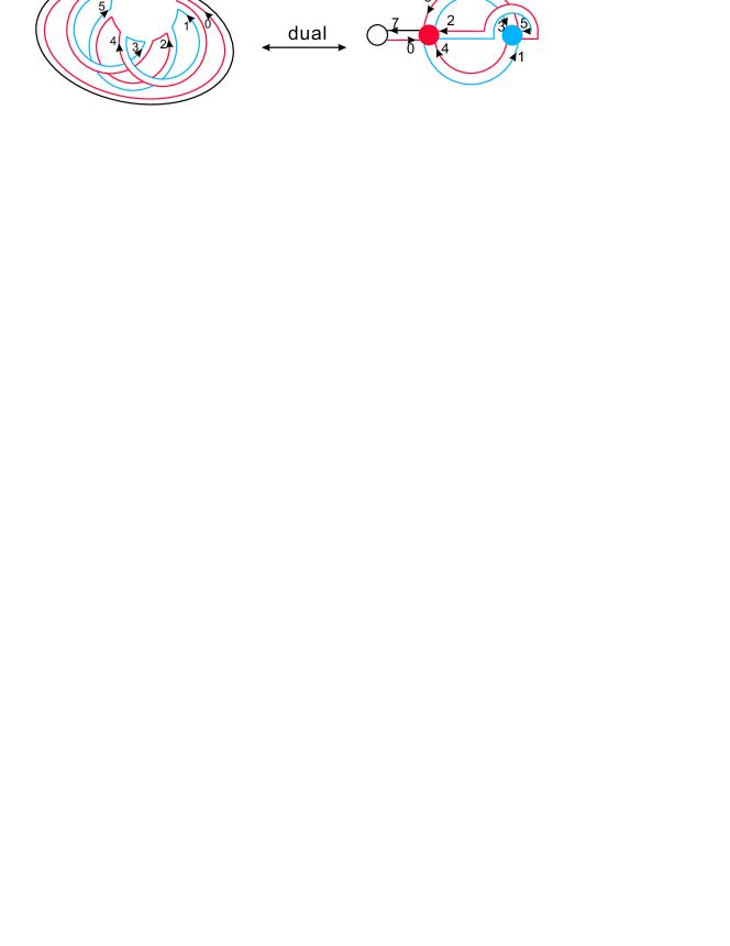
Figure 5: The Poincaré dual: we map a fatgraph with $1$ vertex and $3$ boundary components into a fatgraph with $3$ vertexes and $1$ boundary component.

Given a unicellular map the permutation $\sigma$ and $\gamma$ induces two linear orders of half-edges

$$r<_{\gamma}<\gamma(r)<_{\gamma}\dots<_{\gamma}\gamma^{2n-1}(r),\quad r<_{\sigma}<\sigma(r)<_{\sigma}\dots<_{\sigma}\sigma^{k}(r).$$

Let $a_{1}$ and $a_{2}$ be two distinct half-edges in $\mathfrak{m}$. Then $a_{1}<_{\gamma}a_{2}$ expresses the fact that $a_{1}$ appears before $a_{2}$ in the boundary component $\gamma=\alpha\circ\sigma$. Suppose two half-edges $a_{1}$ and $a_{2}$ belong to the same vertex $v$. Note that $v$ is effectively a cycle which we assume to originate with the first half-edge along which one enters $v$ traveling $\gamma$. Then $a_{1}<_{\sigma}a_{2}$ expresses the fact that $a_{1}$ appears (counterclockwise) before $a_{2}$.

The Poincare-dual maps the rainbow into a distinguished vertex of degree one and provides thereby a natural origin for the cycle $\gamma$. We call this vertex the plant, see Figure 5. Given a unicellular map we call a half-edge the minimum half-edge of a vertex $v$ if it is the first half-edge via which $\gamma$ visits $v$.

2.3 Genus induction

In this section we present a construction of [16], which plays a key role for our main result. It consists of two processes: a slicing-map $\Xi$ and a gluing-map $\Lambda$, which, when restricted to the proper classes, are inverse to each other.

The slicing process splits a vertex into $(2g+1)$ vertices and thereby reduces the genus of the map by $g$. Gluing is effectively inverse to slicing, namely: gluing any $(2g+1)$ vertices in a unicellular map increases the genus of the map by $g$. Slicing and gluing preserve unicellularity.

Definition 3.

A half-edge $h$ is an up-step if $h<_{\gamma}\sigma(h)$, and a down-step if $\sigma(h)\leq_{\gamma}h$. $h$ is called a trisection if $h$ is a down-step and $\sigma(h)$ is not the minimum half-edge of its respective vertex.

The number of trisections in a unicellular map of genus $g$ is given by the following lemma:

Lemma 1.

[16] Let $\mathfrak{m}$ be a unicellular map of genus $g$. Then $\mathfrak{m}$ has exactly $2g$ trisections.

Given a unicellular map $\overline{\mathfrak{m}}$ and a vertex $\overline{v}$ together with a trisection $\tau$ contained in $\overline{v}$. Let $a_{1}$ be the minimum half-edge of $\overline{v}$. Then set $a_{3}=\overline{\sigma}(\tau)$ and $a_{2}$ to be the smallest half-edge between $a_{1}$ and $a_{3}$ (with respect to the order $<_{\overline{\sigma}}$) such that $a_{2}>_{\overline{\gamma}}$.

Since $\tau$ is a trisection such an $a_{2}$ exists. Then we refer to the replacement of

$$\overline{v}=(a_{1},h_{2}^{1},\ldots,h_{2}^{m_{2}},a_{2},h_{3}^{1},\ldots,h_{3}^{m_{3}},a_{3},h_{1}^{1},\ldots,h_{1}^{m_{1}})$$

by the three vertices where $v_{i}=(a_{i},h_{i},^{1},\ldots,h_{i}^{m_{i}})$, $i=1,2,3$, see Figure 6, as slicing. Slicing produces the unicellular fatgraph $\overline{\mathfrak{m}}=(H,\overline{\sigma},\alpha)$.

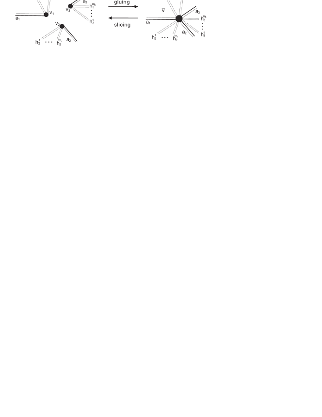
Figure 6: Illustration of gluing and slicing in a unicellular map.

Conversely, let $\mathfrak{m}$ be a unicellular map and let $a_{1}$, $a_{2}$ and $a_{3}$ be three half-edges belonging to three distinct vertices, $v_{i}=(a_{i},h_{i},^{1},\ldots,h_{i}^{m_{i}})$ for some $m_{i}\geq 0$ and $i=1,2,3$. Furthermore suppose $a_{1}<_{\gamma}a_{2}<_{\gamma}a_{3}$.

Then, replacing the cycles $v_{1}$, $v_{2}$ and $v_{3}$ by the cycle

$$\overline{v}=(a_{1},h_{2}^{1},\ldots,h_{2}^{m_{2}},a_{2},h_{3}^{1},\ldots,h_{3}^{m_{3}},a_{3},h_{1}^{1},\ldots,h_{1}^{m_{1}}),$$

is referred to as gluing. Gluing produces the unicellular fatgraph $\overline{\mathfrak{m}}=(H,\overline{\sigma},\alpha)$, see Figure 6, in which the half-edge $\overline{\sigma}^{-1}(a_{3})$ is, by construction, a trisection.

Lemma 2.

[16] Slicing maps a unicellular map together with a trisection into a unicellular map together with three labeled vertices. Gluing maps a unicellular map together with three labeled vertices into a unicellular maps with a trisection.

Suppose we slice $(\overline{\mathfrak{m}},\tau)$ into $(\mathfrak{m},v_{1},v_{2},v_{3})$, where in $\overline{\mathfrak{m}}$ holds $a_{1}<_{\overline{\gamma}}a_{3}<_{\overline{\gamma}}a_{2}$. Then we observe that in $\mathfrak{m}$ $a_{1}$ remains minimum in its new vertex and so does $a_{2}$, because $a_{2}$ is by definition the minimum half-edge where $a_{3}<_{\overline{\gamma}}a_{2}$. However, $a_{3}$ becomes either the minimum half-edge, or remains a half-edge following a trisection. This gives rise to two types of trisections:

Definition 4.

Let $\overline{\mathfrak{m}}$ be a unicellular map and $\overline{v}$ a vertex containing a trisection $\tau$. Slicing $(\overline{\mathfrak{m}},\tau)$ we obtain $(\mathfrak{m},v_{1},v_{2},v_{3})$. If the minimum half-edge of $v_{3}$, denoted by $a_{3}$ is the half-edge $\overline{\sigma}(\tau)$ in $\overline{\mathfrak{m}}$, we call the trisection $\tau$ to be of type I and type II, otherwise.

Proposition 1.

Let $\mathfrak{m}_{g}$ denote a unicellular map of genus $g$ having $n$ edges. Let furthermore $\tau^{I}$ denote a trisection of type I and $\tau^{II}$ denote a trisection of type II. Then we have the mappings $\Phi$ and $\Psi$:

$$\Phi(\mathfrak{m}_{g},v_{1},v_{2},v_{3})=(\mathfrak{m}_{g+1},\tau^{I}),\quad\Psi(\mathfrak{m}_{g},v_{1},v_{2},\tau)=(\mathfrak{m}_{g+1},\tau^{II})$$

are bijections, where $v_{1}$, $v_{2}$ and $v_{3}$ denote three distinct vertices in $\mathfrak{m}_{g}$ and $\mathfrak{m}_{g+1}$ is a unicellular map of genus $g+1$ having $n$ edges.

Here $\Phi$ generates the trisection $\tau^{I}$ in a unicellular map of genus $g+1$ and the trisection $\tau^{II}$ persists when applying the mapping $\Psi$.

Gluing can be described as follow:
Given a unicellular map of $\mathfrak{m}_{g-k}$, together with a sequence of vertices $V=\{v_{1},\ldots v_{2k+1}\}$, where $v_{i}<_{\gamma}v_{i+1}$, $\forall 1\leq i<2k+1$. Then:
I. we glue the last three vertices $v_{2k-1}$, $v_{2k}$ and $v_{2k+1}$ via $\Phi$, thereby obtaining the unicellular map $\mathfrak{m}_{g-k+1}$ together with trisection $\tau^{I}$.
II. we apply $\Psi(\mathfrak{m}_{g-k+i},v_{2k-2i-1},v_{2k-2i},\tau^{I})$ $k-1$ times for $i=1$ to $i=k-1$. This produces the unicellular map $\mathfrak{m}_{g}(n)$, together with a trisection $\tau^{II}$. The process defines a mapping

$$\Lambda(\mathfrak{m}_{g-k},v_{1},\ldots,v_{2k+1})=(\mathfrak{m}_{g},\tau),$$

where we do not label $\tau$ by type since in general we do not know whether $\Psi$ has been applied. The order of the vertices in $V$ is given by the partial order determined by $\gamma$. Thus $V$ can be considered as a set of vertices in $\mathfrak{m}_{g-k}$, ordered by $<{\gamma}$. $\Lambda$ merges vertices from right to left by first applying $\Phi$ once then applying $\Psi$ several times.

$\Lambda$ is reversed as follows: given a unicellular map $\mathfrak{m}_{g}$ of genus $g$ and $i=0$:
1. if $\tau$ is type II trisection in $\mathfrak{m}_{g-i}$, then let $(\mathfrak{m}_{g-i-1},v_{2i+1},v_{2i+2},\tau)=\Psi^{-1}(\mathfrak{m}_{g-i},\tau)$. We increase $i$ to $i+1$ and repeat step 1.
3. if $\tau$ has type I, let $(\mathfrak{m}_{g-i},v_{2i+1},v_{2i+2},v_{2i+3})=\Phi^{-1}(\mathfrak{m}_{g-i-1},\tau)$.
Then we return

$$\Xi(\mathfrak{m}_{g},\tau)=(\mathfrak{m}_{g-i},V_{\tau}).$$

By construction, $\Lambda$ and $\Xi$ are inverse to each other.

Theorem 1.

[16] Let $U_{g}^{t}$ denote the set of tuples $(\mathfrak{m}_{g},v_{1},\ldots,v_{t})$, where $v_{1},\ldots,v_{t}$ is a sequence of vertices in $\mathfrak{m}_{g}$. Furthermore, let $D_{g}$ denote the set of tuples $(\mathfrak{m}_{g},\tau)$, where $\tau$ is a trisection of $\mathfrak{m}_{g}$. Then

$$\Lambda\colon{\dot{\bigcup}}_{k=0}^{g-1}U_{k}^{2g-2k+1}\rightarrow D_{g},\quad\Xi\colon D_{g}\rightarrow{\dot{\bigcup}}_{k=0}^{g-1}U_{k}^{2g-2k+1}$$

are bijections and $\Lambda\circ\Xi=\text{\rm id}$ and $\Xi\circ\Lambda=\text{\rm id}$.

Let $\epsilon_{g}(n)$ denote the number of unicellular map of genus $g$ having $n$ edges. Then we have the following enumerative corollary

Corollary 1.

$$2g\cdot\epsilon_{g}(n)={n+1-2(g-1)\choose 3}\epsilon_{g-1}(n)+\cdots+{n+1\choose 2g+1}\epsilon_{0}(n).$$ (4)

Here the $2g$-factor on left hand side counts the number of trisection in $\mathfrak{m}_{g}$ and the binomial coefficients on the right hand side counts the number of distinct selections of subsets of $(2k+1)$ vertices from a unicellular map $\mathfrak{m}_{g-k}$.

Iterating $\Xi$, we obtain

$$\epsilon_{g}(n)=\sum_{0=g_{0}<g_{1}<\cdots<g_{r}=g}\prod_{i=1}^{r}\frac{1}{2g_{i}}{n+1-2g_{i-1}\choose 2(g_{i}-g_{i-1})+1}\cdot\epsilon_{0}(n),$$ (5)

where $\epsilon_{0}(n)$ is the number of planar trees having $n$ edges, i.e. the Catalan number $\frac{1}{n+1}{2n\choose n}$.

3 Uniform generation of matchings

In this section, we show how to generate a matching of a given genus $g$ over $2n$ vertices with uniform probability.

Any unicellular map $\mathfrak{m}_{g}$ together with one of its $2g$ trisections is mapped via $\Xi$ into a unicellular map of lower genus. Note that the genus decreases at least by one. Therefore, by iterating the process finitely many times (at most $g$), we arrive at a unicellular map of genus $0$, i.e a planar tree.

For our construction it is important to keep track of the particular slicing process. Accordingly, we introduce slice/glue paths as follows.

Definition 5.

Suppose $\mathfrak{m}_{g}$ is a unicellular map of genus $g$ having $n$ edges. Then a sequence unicellular maps

$$(\mathfrak{m}^{0}=\mathfrak{m}_{g_{0}=0},\mathfrak{m}^{1}=\mathfrak{m}_{g_{1}},\ldots,\mathfrak{m}^{r}=\mathfrak{m}_{g_{r}=g})$$

is called a slice path from $\mathfrak{m}_{g}$ to $\mathfrak{m}_{0}$ and a glue path when considered from $\mathfrak{m}_{0}$ to $\mathfrak{m}_{g}$, where $\Xi(\mathfrak{m}_{g_{i}},\tau_{i})=(\mathfrak{m}_{g_{i-1}},V_{g_{i-1}})$ holds for some $\tau_{i}$ in $\mathfrak{m}_{g_{i}}$, $0<i\leq r$.

We next consider $P_{g}(\mathfrak{m}^{0})$, the set of distinct glue paths from a given $\mathfrak{m}^{0}=\mathfrak{m}_{0}$ to some unicellular maps of fixed genus $g$.

Lemma 3.

The cardinality of $P_{g}(\mathfrak{m}^{0})$ is given by

$$\sum_{0=g_{0}<g_{1}<\cdots<g_{r}=g}\prod_{i=1}^{r}\frac{1}{2g_{i}}{n+1-2g_{i-1}\choose 2(g_{i}-g_{i-1})+1}.$$

Proof.

In order to construct $\mathfrak{m}_{g_{i}}$ from $\mathfrak{m}_{g_{i-1}}$, $0<i\leq r$, we need to select $2(g_{i}-g_{i-1})+1$ vertices from $\mathfrak{m}_{g_{i-1}}$.

Euler characteristic shows that there are $(n+1-2g_{i-1})$ distinct vertices in $\mathfrak{m}_{g_{i-1}}$, whence there are ${n+1-2g_{i-1}\choose 2(g_{i}-g_{i-1})+1}$ ways to select a subset of vertices $V_{g_{i-1}}$.

On the other hand, the mapping $\Lambda$ produces $\mathfrak{m}_{g_{i}}$ with a labeled trisection $\tau_{i}$, i.e., the same $\mathfrak{m}_{g_{i}}$ will be produced exactly $2g_{i}$ times. Accordingly, we need to normalize the production by a factor $1/2g_{i}$ for each application of $\Lambda$.

As a result the total number of glue paths in $P_{g}(\mathfrak{m}^{0})$ is

$$\sum_{0=g_{0}<g_{1}<\cdots<g_{r}=g}\prod_{i=1}^{r}\frac{1}{2g_{i}}{n+1-2g_{i-1}\choose 2(g_{i}-g_{i-1})+1},$$

which is exactly the coefficient of $\epsilon_{0}(n)$ in eq. (5). ∎

The problem of generating a unicellular map of genus $g$ having $n$ edges with uniform probability thus splits into two parts: we first generate a planar tree $\mathfrak{m}_{0}$ with $n$ edges with uniform probability. Second we generate a glue path from $P_{g}(\mathfrak{m}^{0})$ with uniform probability. It is well-known how to implement the first step by a linear time (rejection) sampler [22] and it thus remains to present an algorithm for the second step.

We construct a glue path inductively. Suppose we are at step $i$ and we have constructed a unicellular map $\mathfrak{m}^{i}$ of genus $g_{i}$. Then the next genus $g_{i+1}$ is suggested by the process ${\tt NextGenus}$. This process considers the sequence of genus $g_{0},\ldots,g_{i}$ and the target genus $g$ as input, and returns the genus $g_{i+1}$. Let $\mathbb{P}(g_{i+1}=t\mid g_{0},\ldots,g_{i},g)$ denote the probability of $g_{i+1}$ equals $t$ under the condition that $g_{0},\ldots,g_{i}$ are the genus of the previous steps and $g$ is the target genus. Then

$$\mathbb{P}(g_{i+1}=t\mid g_{0},\ldots,g_{i},g)=\frac{\sum\limits_{t_{0}=g_{0},\ldots,t_{i}=g_{i},g_{i+1}=t<t_{i+1}<\cdots<t_{r}=g}\prod\limits_{i=1}^{r}\frac{1}{2t_{i}}{n+1-2t_{i-1}\choose 2(t_{i}-t_{i-1})+1}}{\sum\limits_{t_{0}=g_{0},\ldots,t_{i}=g_{i}<\cdots<t_{r}=g}\prod\limits_{i=1}^{r}\frac{1}{2t_{i}}{n+1-2t_{i-1}\choose 2(t_{i}-t_{i-1})+1}}.$$ (6)

Next we select the sequence of vertices from $\mathfrak{m}^{i}$ by process SelectVertex. This process chooses vertices in $2(g_{i+1}-g_{i})+1$ independent steps. The probability of a vertex being selected is given by $1/(n+2-2g_{i}-k)$, where $(n+2-2g_{i}-k)$ is the number of remaining non-selected vertices in the $k$th step, $1\leq k\leq 2(g_{i+1}-g_{i})+1$. Since the selected vertices are ordered automatically by $<_{\gamma_{\mathfrak{m}^{i}}}$, the same set is generated with multiplicity $(2(g_{i+1}-g_{i})+1)!$. Normalizing the resulting term by the factor $1/(2(g_{i+1}-g_{i})+1)!$, the probability of the set $V_{i}$, $0\leq i<r$ is given by

$$\mathbb{P}_{\tt Select}(V_{i})=\frac{1}{(2(g_{i+1}-g_{i})+1)!}\cdot\frac{1}{n+1-2g_{i}}\cdots\frac{1}{n-2g_{i+1}}=\frac{1}{{n+1-2g_{i}\choose 2(g_{i+1}-g_{i})+1}}.$$ (7)

After the sequence of vertices $V_{i}$ is selected, a unicellular map $\mathfrak{m}^{i+1}$ is constructed by the process Glue, applying mapping $\Lambda$. We present the pseudocode of the procedures in Algorithm 1.

1:  UniformMatching ($\mathfrak{m}^{0},TargetGenus$)

2:  $i\leftarrow 0$

3:  while $g_{i}\leq TargetGenus$ do

4:     $g_{i+1}\leftarrow{\tt NextGenus}~{}(g_{0},\ldots,g_{i},TargetGenus)$

5:     $V_{i}\leftarrow{\tt SelectVertex}~{}(\mathfrak{m}^{i},2(g_{i+1}-g_{i})+1)$

6:     $\mathfrak{m}^{i+1}\leftarrow{\tt Glue}~{}(\mathfrak{m}^{i},V_{i})$

7:     $i\leftarrow i+1$

8:  end while

9:  return $\mathfrak{m}^{i}$

Algorithm 1

Assuming the target genus to be constant and taking into account that during our construction the genus is strictly increasing, the while-loop of Algorithm 1 is executed only a constant number of times. Using appropriate memorization techniques, NextGenus and Glue can be implemented in constant time and SelectVertex in linear time. Thus, combined with a linear time sampler for planar trees, our approach allows for the uniform generation of random matchings in time $O(n)$.

Lemma 4.

Given a planar tree $\mathfrak{m}^{0}$ with $n$ edges and a genus $g$, the probability of a glue path $p_{g}$ generated by Algorithm 1 is $\epsilon_{0}(n)/\epsilon_{g}(n)$.

Proof.

Assume a glue path

$$p_{g}=\{\mathfrak{m}^{0}=\mathfrak{m}_{g_{0}=0},\mathfrak{m}^{1}=\mathfrak{m}_{g_{1}},\ldots,\mathfrak{m}^{r}=\mathfrak{m}_{g_{r}=g}\}$$

is generated by Algorithm 1. Since for each step, the process of choosing the genus for the next step and selecting labeled vertices is independent, the probability of $P_{g}$ is given by

$$\mathbb{P}(P_{g})=\prod_{i=0}^{r-1}\mathbb{P}(g_{i+1}=t_{i+1}|g_{0},\ldots,g_{i},g)\cdot\mathbb{P}(V_{i}).$$

We substitute eq. (6) and eq. (7) and obtain

$$\mathbb{P}(P_{g}) = \prod_{i=0}^{r-1}\frac{\sum_{t_{0}=g_{0},\ldots,t_{i}=g_{i},g_{i+1}=t<t_{i+1}<\cdots<t_{r}=g}\prod_{i=1}^{r}\frac{1}{2t_{i}}{n+1-2t_{i-1}\choose 2(t_{i}-t_{i-1})+1}}{\sum_{t_{0}=g_{0},\ldots,t_{i}=g_{i}<\cdots<t_{r}=g}\prod_{i=1}^{r}\frac{1}{2t_{i}}{n+1-2t_{i-1}\choose 2(t_{i}-t_{i-1})+1}}\cdot\frac{1}{{n+1-2g_{i}\choose 2(g_{i+1}-g_{i})+1}}$$

$$= \frac{\prod_{t_{1}=g_{1},\ldots,t_{r}=g_{r}}\frac{1}{2t_{i}}{n+1-2t_{i-1}\choose 2(t_{i}-t_{i-1})+1}}{\sum_{0=t_{0}<\cdots<t_{r}=g}\prod_{i=1}^{r}\frac{1}{2t_{i}}{n+1-2t_{i-1}\choose 2(t_{i}-t_{i-1})+1}}\cdot\prod_{i=0}^{r-1}\frac{1}{{n+1-2g_{i}\choose 2(g_{i+1}-g_{i})+1}}$$

$$= \frac{1}{\sum_{0=t_{0}<\cdots<t_{r}=g}\prod_{i=1}^{r}\frac{1}{2t_{i}}{n+1-2t_{i-1}\choose 2(t_{i}-t_{i-1})+1}}$$

$$= \frac{\epsilon_{0}(n)}{\epsilon_{0}(n)\cdot\sum_{0=t_{0}<\cdots<t_{r}=g}\prod_{i=1}^{r}\frac{1}{2t_{i}}{n+1-2t_{i-1}\choose 2(t_{i}-t_{i-1})+1}}$$

$$= \frac{\epsilon_{0}(n)}{\epsilon_{g}(n)},$$

whence the lemma. ∎

Corollary 2.

Suppose a planar tree $\mathfrak{m}^{0}$ is uniformly generated, i.e., with probability $1/\epsilon_{0}(n)$. Then a unicellular map $\mathfrak{m}^{r}=\mathfrak{m}_{g}$ is uniformly generated by Algorithm 1 with probability $1/\epsilon_{g}(n)$.

4 Uniform generation of diagrams

In this section, we extend our result of Section 3 in order to generate diagrams of genus $g$ with uniform probability. The idea is to uniformly generate first a matching of genus $g$ with $n$ arcs. In a second step we choose $(\ell-2n)$ unpaired vertices and insert them into the matching.

Let $\mathbb{P}_{d}(t=n|\ell,g)$ denote the probability of the diagram having exactly $n$ arcs, $0\leq n\leq\lfloor\ell/2\rfloor$. In the following we compute $\mathbb{P}_{d}(t=n|\ell,g)$.

Let $\delta_{g}(\ell)$ denote the number of diagrams of genus $g$ over $\ell$ vertices. Furthermore, let $\delta_{g}(\ell,n)$ denote the number of diagrams of genus $g$ over $\ell$ vertices having exactly $n$ arcs, $2n\leq\ell$. Then $\ell-2n$ vertices are unpaired and

$$\delta_{g}(\ell,n)={\ell\choose\ell-2n}\epsilon_{g}(n).$$

Furthermore

$$\delta_{g}(\ell)=\sum_{n=0}^{\lfloor l/2\rfloor}\delta_{g}(\ell,n)=\sum_{n=0}^{\lfloor l/2\rfloor}{\ell\choose\ell-2n}\epsilon_{g}(n).$$ (8)

In order to generate a diagram of genus $g$ over $\ell$ arcs uniformly, we need to solve

$$\frac{1}{\delta_{g}(\ell)}=\mathbb{P}_{d}(t=n|\ell,g)\cdot\frac{1}{\epsilon_{g}(n)}\cdot\frac{1}{{\ell\choose\ell-2n}},$$

whence $\mathbb{P}_{d}(t=n|\ell,g)=\delta_{g}(\ell,n)/\delta_{g}(\ell)$.

We present the pseudocode of UniformDiagram as Algorithm 2. The subroutine NumberofArcs returns $n$ with probability $\mathbb{P}_{d}(t=n|\ell,g)$, which determines the number of arcs in diagram $D_{g}(\ell)$. UnifomTree is a standard process uniformly generating a matching of genus $0$ with $n$ arcs. Finally, the process InsertUnpairedVertices first chooses $(\ell-2n)$ vertices from $\ell$ vertices as unpaired. It leaves $2n$ vertices not selected, which are considered to be paired. Then the process maps the $2n$ vertices of the matching generated by UniformMatching and keeps the arcs in the upper half-plane. Accordingly, a diagram of genus $g$ over $\ell$ vertices with exactly $n$ arcs is generated. The result of some experiments conducted in connection with the generation of random matchings and diagrams using our algorithms is shown in Figure 7.

1:  UniformDiagram ($\ell,TargetGenus$)

2:  $n\leftarrow{\tt NumberofArcs}(\ell,g)$

3:  $\mathfrak{m}_{0}\leftarrow{\tt UnifomTree}(n)$

4:  $\mathfrak{m}_{g}\leftarrow{\tt UniformMatching}(\mathfrak{m},TargetGenus)$

5:  $D_{g}\leftarrow{\tt InsertUnpairedVertices}(\mathfrak{m}_{g},\ell)$

6:  return $D_{g}$

Algorithm 2

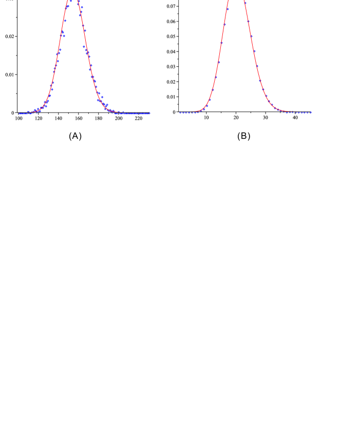
Figure 7: Uniform generation: (A) matchings, $n=12$, $g=2$ and $\epsilon_{2}(n/2)=6468$. We generate $N=10^{6}$ matchings and display the frequencies of their multiplicities (blue dots) together with the binomial coefficient of the uniform sampling ${N\choose\ell}(1/\epsilon_{2}(n/2))^{\ell}(1-1/\epsilon_{2}(n/2))^{N-\ell}$ (red). (B) The analog of (A) for diagrams. Here we have $n=12$, $g=2$ and $\delta_{2}(n)=48741$. We generate $N=10^{6}$ diagrams and display the frequencies of their multiplicities (blue dots) together with the binomial coefficients ${N\choose\ell}(1/\delta_{2}(n))^{\ell}(1-1/\delta_{2}(n))^{N-\ell}$ (red).

5 Non-uniform sampling

RNA structures can be represented as diagrams and are, due to the biophysical context subject to certain constraints with respect to their free energy [23]. The latter energy is oftentimes modeled as a function of the loops of the underlying RNA structure [23], $S$. These loops are in fact equal to the boundary components of the fatgraph constructed from the molecule. In the following we shall discuss, $\eta(S)$, a simplified version of the actual bio-physical loop-energy of a structure $S$.

Let us start with RNA secondary structures, that correspond to diagrams of genus $0$. For a secondary structure $S_{0}$, we denote its corresponding (see Section 2, duality mapping $\pi$) unicellular map by $\mathfrak{m}_{0}=\pi(S_{0})$. The bonds or arcs of the structure then correspond to edges of the unicellular map $\mathfrak{m}_{0}$ and loops or boundary components to vertices. Three types of loops are distinguished: hairpin loops, interior loops (including helices and bludge loops) and multi-loops. Accordingly, the duality maps hairpin loops into vertices of degree one, interior loops into vertices of degree two, and multi-loop into vertices of degree greater than two, see Figure 8. $\eta(S)$ extends these types in order to deal with structures having arbitrary genus $g\geq 0$ as follows.

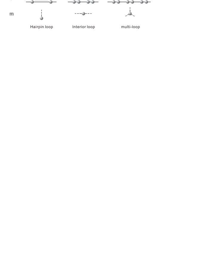
Figure 8: Hairpin loops, interior loops and multi-loops in secondary structures and their translation into unicellular maps.

Let $S_{g}$ denote an RNA structure having length $\ell$, $n$ arcs and genus $g$, and $\mathfrak{m}_{g}=\pi(S_{g})$ its corresponding unicellular map. Then $\eta(S_{g})$ is given by

$$\eta(S_{g})=n\cdot b+\sum_{v\in\mathbb{V}}T(v)+L^{pk}_{g}.$$ (9)

Here $b$ represents an energy contribution of arcs, $\mathbb{V}$ the set of all vertices $\mathfrak{m}_{g}$, $T(v)$ is function given by

$$T(v)=\begin{cases}L^{hp}\quad\text{if $d(v)=1$},\\ L^{int}\quad\text{if $d(v)=2$},\\ L^{mul}\quad\text{if $d(v)>2$ and $v$ has no trisection,}\\ 0\quad\text{if $v$ is attached to the root,}\end{cases}$$

where $d(v)$ is the degree of vertex $v$, and $L^{X}$ is the contribution of a loop of type $X$, where $X=\{hp,int,mul\}$. Finally, $L^{pk}_{g}$ represents a contribution that stems from novel loop-types emerging for genus $g>0$. In this model, we do not take contributions from unpaired vertices into account.

In case of $g=1$, there are four different types of pseudoknots [24], see Figure 9. This is analogous for any genus: there are always only finitely many corresponding shadows [25, 24], see Figure 9. Here, a shadow is a diagram without unpaired vertices in which all stacks (parallel arcs) have size one. Formally, a shadow of a structure can be obtained by first removing all its unpaired vertices, second removing all noncrossing arcs (together with their vertices) and then replacing a set of parallel arcs (and the incident vertices) of the form $\{(i,j),(i+1,j-1),\ldots,(i+\ell-1,j-\ell+1)\}$ by a single arc (and two vertices).

Let us have a closer look at the boundary components of these shadows in case of genus $1$. (H) is inspected to have one boundary component, whence $\eta(S_{\text{H}})=2b+L^{mul}+L^{pk}_{1}$. (K) and (L) have two boundary components and accordingly $\eta(S_{\text{K}})=\eta(S_{\text{L}})=3b+2L^{mul}+L^{pk}_{1}$. Finally, for (M) we have $\eta(S_{\text{M}})=4b+3L^{mul}+L^{pk}_{1}$.

Consider a matching $S_{1}$ of genus $1$ having $n$ arcs and $\mathfrak{m}_{1}=\pi(S_{1})$ the unicellular map given by the duality. By selecting a trisection $\tau$ in $\mathfrak{m}_{1}$ and applying the mapping $\Xi$, we obtain $\Xi(\mathfrak{m}_{1},\tau)=(\mathfrak{m}_{0},v_{1},v_{2},v_{3})$ and three labeled vertices. Here we write $\mathfrak{m}_{0}^{(3)}=(\mathfrak{m}_{0},v_{1},v_{2},v_{3})$ for short. Let $S_{0}^{(3)}$ denote a secondary structure with three labeled boundary component where $\pi(S_{0}^{(3)})=\mathfrak{m}_{0}^{(3)}$. Let further $\mathbb{S}_{0,n}^{(3)}$ and $\mathbb{S}_{1,n}$ denote the set of $S_{1}$ and $S_{0}^{(3)}$ respectively. By Lemma 1, there are two trisections in $\mathfrak{m}_{1}$. Therefore, by selecting the same $S_{1}$ and different trisection $\tau$, $\Xi$ results in different $S_{0}^{(3)}$. Thus we have the cardinality $2|\mathbb{S}_{1,n}|=|\mathbb{S}_{0,n}^{(3)}|$. Figure 9 shows this for the four shadows of genus $1$ and their secondary structure with three labeled boundary components.

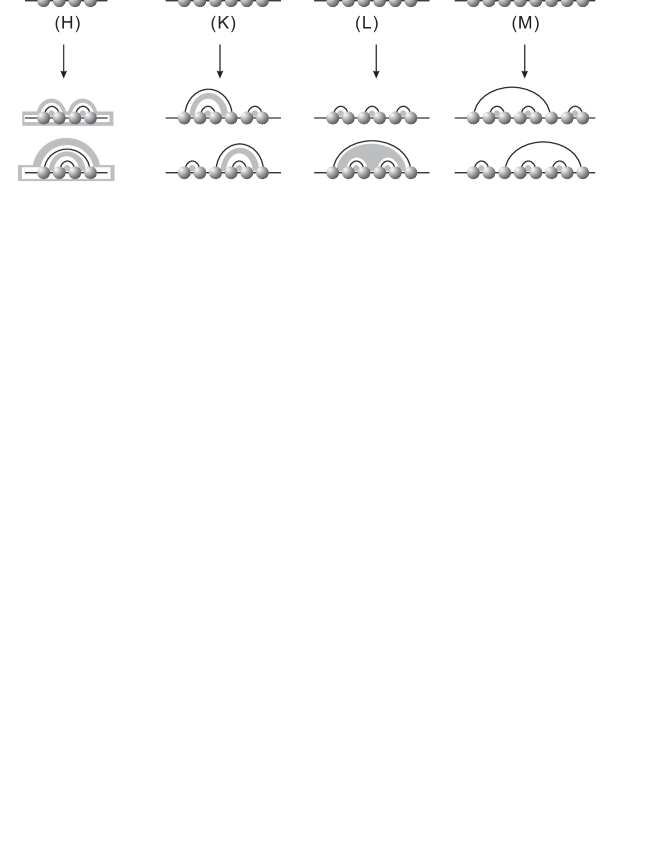
Figure 9: Correspondence between shadows of genus one and their labeled secondary structures.

We next formulate an “energy” for structures $S_{0}^{(3)}$, $\eta(S_{0}^{(3)})$, that matches the energy $\eta$ for their corresponding counterpart of genus one after gluing. Note that this allows us to reduce everything to secondary structures with three labeled boundary components. To this end, let $v_{1}$, $v_{2}$ and $v_{3}$ be three labeled vertices in $\mathfrak{m}_{0}^{(3)}$, where $\mathfrak{m}_{0}^{(3)}=\pi(S_{0}^{(3)})$. Setting $T(v_{1})=T(v_{2})=T(v_{3})=(L_{1}^{pk}+L^{mul})/3$ we observe

Proposition 2.

We have $\eta(S_{1})=\eta(S_{0}^{(3)})$.

Proof.

The mapping $\Xi$ is a bijection and $\Lambda(\mathfrak{m}_{0},v_{1},v_{2},v_{3})=(\mathfrak{m}_{1},\tau)$. The three labeled vertices in $\mathfrak{m}_{0}$ are glued as $\overline{v}$, where $d(\overline{v})\geq 3$. Hence $T(\overline{v})=L^{mul}+L^{pk}_{1}=T(v_{1})+T(v_{2})+T(v_{3})$, because $T(v_{1})=T(v_{2})=T(v_{3})=(L^{pk}_{1}+L^{mul})/3$. The other vertices in $\mathfrak{m}_{0}$ maintain hence their scores are not changed. ∎

Given $\eta(S)$ we proceed along the lines of [26] and construct a probability space of structures by computing the partition function of a given sequence. Let $\theta(n)=\sum_{S\in\mathbb{S}_{n}}e^{\eta(S)}$ denote the total energy of all structures. A structure, $S$, is sampled with probability $e^{\eta(S)}/\theta(n)$. In case of secondary structures, loop-based and arc-based energy models are compatible to the standard recursion of secondary structure [27] and $\theta_{0}(n)$ can be computed by the recursion

$$\theta(n)=\sum_{i=1}^{n-2}\theta(i)\theta(n-i-1)+e^{{L^{hp}}+b}\cdot\theta(1)+e^{{L^{int}}+b}\cdot\theta(n-1)+e^{{L^{mul}}+b}\cdot\sum_{i=1}^{n-3}\theta(i)\theta(n-i-2),$$

where $\eta$ is the energy functional, discussed above. As there is only one summation in the above recursion, $\theta(n)$ is computed in $O(n^{2})$ time.

We proceed by showing that the new functional, $\eta(S_{0}^{(3)})$, is also compatible with the secondary structure recursions.

Lemma 5.

Let $\theta_{1}(n)=\sum_{S\in\mathbb{S}_{1,n}}e^{\eta(S)}$ and $\theta_{0}^{(3)}(n)=\sum_{S\in\mathbb{S}_{0,n}^{(3)}}e^{\eta(S)}$. Then $\theta_{1}(n)=\theta_{0}^{(3)}(n)/2$ can be computed in $O(n^{2})$ time. Once $\theta_{1}(n)$ is computed, a structure of genus one, $S_{1}$, is sampled with probability $e^{\eta(S_{1})}/\theta_{1}(n)$ in $O(n)$ time.

Proof.

We have $\eta(S_{1})=\eta(S_{0}^{(3)})$ for all $S_{1}\in\mathbb{S}_{1,n}$ and $S_{0}^{(3)}\in\mathbb{S}_{0,n}^{(3)}$, and $2|\mathbb{S}_{1,n}|=|\mathbb{S}_{0,n}^{(3)}|$. Therefore,

$$\theta_{1}(n)=\sum_{S\in\mathbb{S}_{1,n}}e^{\eta(S)}=\frac{1}{2}\sum_{S\in\mathbb{S}_{0,n}^{(3)}}e^{\eta(S)}=\frac{1}{2}\theta_{0}^{(3)}(n).$$

We next show that $\theta_{0}^{(3)}(n)$ can be computed in $O(n^{2})$ time. Let $\theta_{0}^{(2)}=\sum_{S\in\mathbb{S}_{0,n}^{(2)}}e^{\eta(S)}$ and $\theta_{0}^{(1)}=\sum_{S\in\mathbb{S}_{0,n}^{(1)}}e^{\eta(S)}$, where $\mathbb{S}_{0,n}^{(2)}$ and $\mathbb{S}_{0,n}^{(1)}$ denote the sets of secondary structures with two and one labeled boundary components. The functionals of these labeled boundary components are computed exactly as in the case of $S_{0}^{(3)}$.

Then we have, see also Figure 10:

$$\theta_{0}^{(3)}(n) = 2\sum_{i=1}^{n-2}\theta_{0}^{(3)}(i)\theta_{0}(n-i-1)+2\sum_{i=1}^{n-2}\theta_{0}^{(2)}(i)\theta_{0}^{(1)}(n-i-1)$$

$$+ e^{(L^{mul}+L_{1}^{pk})/3+b}\cdot\left(2\sum_{i=1}^{n-2}\theta_{0}^{(2)}(i)\theta_{0}(n-i-1)+\sum_{i=1}^{n-2}\theta_{0}^{(1)}(i)\theta_{0}^{(1)}(n-i-1)\right)$$

$$+ 2e^{L^{mul}+b}\cdot\left(\sum_{i=1}^{n-3}\theta_{0}^{(3)}(i)\theta_{0}(n-i-2)+\sum_{i=1}^{n-3}\theta_{0}^{(2)}(i)\theta_{0}^{(1)}(n-i-2)\right)$$

$$+ e^{(L^{mul}+L_{1}^{pk})/3+b}\cdot\left(2\sum_{i=1}^{n-3}\theta_{0}^{(2)}(i)\theta_{0}(n-i-2)+\sum_{i=1}^{n-3}\theta_{0}^{(1)}(i)\theta_{0}^{(1)}(n-i-2)\right)$$

$$+ e^{L^{int}}\cdot\theta_{0}^{(3)}(n-1)+e^{(L^{pk}_{1}+L^{mul})/3+b}\cdot\theta_{0}^{(2)}(n-1).$$

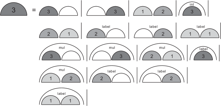
Figure 10: The recursion for $\theta_{0}^{(3)}$.

Analogously, we have recursions for $\theta_{0}^{(2)}(n)$ and $\theta_{0}^{(1)}(n)$, which can be computed in $O(n^{2})$ time. Therefore, $\theta_{1}(n)=\theta_{0}^{(3)}(n)$ can be computed in $O(n^{2})$ time.

In order to sample a diagram of genus $1$ over $\ell$ vertices, $D_{1}$, we need first to determine its number of arcs. As in the case of uniform sampling, we have $\vartheta_{1}(\ell)=\sum_{n=0}^{\lfloor\ell/2\rfloor}\vartheta_{1}(\ell,n)$, where $\vartheta_{1}(\ell,n)={\ell\choose\ell-2n}\theta_{1}(n)$. Replacing in the formulae for uniform sampling $\epsilon_{1}(n)$ by $\theta_{1}(n)$ and $\delta_{1}(n)$ by $\vartheta_{1}(n)$, we find that the probability of sampling a diagram with $n$ arcs is given by $\vartheta_{1}(\ell,n)/\vartheta_{1}(\ell)$. It remains to sample a matching $S_{0}^{(3)}$ with $n$ arcs and to subsequently glue the three labeled vertices in $\mathfrak{m}_{0}^{(3)}=\pi(S_{0}^{(3)})$. This generates a unicellular maps of genus one, $\mathfrak{m}_{1}$, which is associated to $S_{1}=\pi^{-1}(\mathfrak{m}_{1})$ by duality. Note that choosing different slice-paths for $S_{1}$ generates two different $S_{0}^{(3)}$, see eq. (10).

(10)

The probability of a structure of genus one, $S_{1}$, is then given by

$$\frac{2e^{\eta(S_{0}^{(3)})}}{\theta_{0}^{(3)}(n)}=\frac{2e^{\eta(S_{1})}}{2\theta_{1}(n)}=\frac{e^{\eta(S_{1})}}{\theta_{1}(n)}.$$

Finally, we insert the unpaired vertices into $S_{1}$ and obtain $D_{1}$ with the probability

$$\frac{\vartheta_{1}(\ell,n)}{\vartheta_{1}(\ell)}\cdot\frac{{\ell\choose\ell-2n}e^{\eta(D_{1})}}{\theta_{1}(n)}=\frac{e^{\eta(D_{1})}}{\vartheta_{1}(\ell)}.$$

∎

6 Conclusion

In this paper we have proposed an original and highly efficient (linear time) approach to sample random RNA pseudoknotted structures in the uniform and a non-uniform model. The later builds on a simplified concept of free energy, favoring foldings of a native appearance. This is a first step towards efficient prediction algorithms for pseudoknotted RNA since structure predictions of good quality can easily be derived from suitable (high quality) random samples (see [28] and the references given there). To this end, our algorithms need to be extended towards two directions:

1. The probability model needs to be improved further, and

2. the RNA sequence needs to be taken into account.

An immediate application of the uniform sampler are the distributions of loops in structures of genus $g$. We have shown that the loops in structures are translated into vertices of their associated unicellular maps. In particular, a hairpin loop corresponds to a vertex of degree one, an interior loop to a vertex of degree two and a multi-loop is to some vertex having degree greater than two without a trisection. Finally a pseudoknot loop corresponds to a vertex having degree greater than two containing a trisection. In Fig. 11 we present the respective data, filtered by genus.

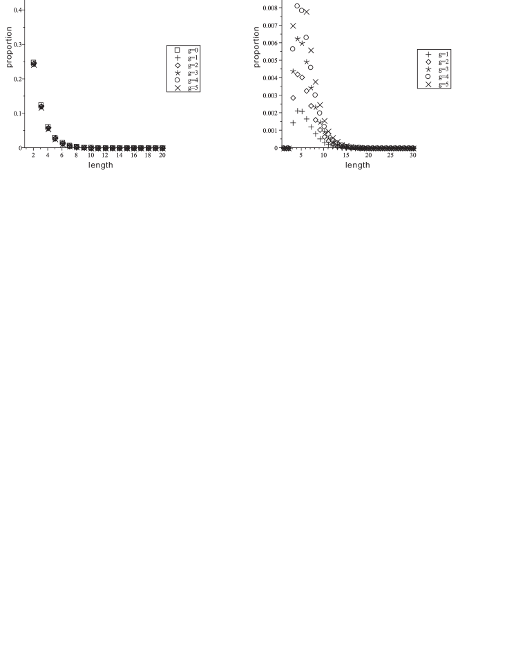
Figure 11: Loops in uniformly generated, genus filtered, RNA structures. Left: distribution of standard loops, where $x$-axis is the length of boundary component and $y$-axis is frequency. Right: distribution of pseudoknot loops.

It is well known in context of pseudoknot-free secondary structures how to use either a sophisticated model for the free energy or stochastic concepts like the maximum likelihood approach to obtain realistic probability models applicable to random sampling. Our approach seems to be suitable to apply the latter and it is a topic for future research to work out the details. Incorporating the sequence is a more complicated task but again results for classic RNA secondary structures prove it feasible with only small losses in efficiency [29].

Thus we assume our findings of this paper an important contribution towards the development of efficient structure prediction tools for pseudoknotted RNA structures. Those are also in need for state of the art tools addressing the inverse folding problem. The latter quite often use some search heuristic (like e.g. a genetic algorithm) to process the space of possible sequences using structure prediction tools to judge the quality (similarity to input) of current solutions. For the large number of calls, the efficiency of the prediction algorithm is crucial for the applicability of the entire approach. Today’s established algorithms for the prediction of pseudoknotted RNA with run times in $O(n^{4})$ or worth (see [9]) seem not to be appropriate.

References

- [1] E. Westhof, L. Jaeger, RNA pseudoknots, Curr. Opin. Struct. Biol. 2 (1992) 327–333.
- [2] A. Loria, T. Pan, Domain structure of the ribozyme from eubacterial ribonuclease, RNA 2 (1996) 551–563.
- [3] D. W. Staple, S. E. Butcher, Pseudoknots: RNA structures with diverse functions, PLoS Biol. 3 (2005) e213.
- [4] D. Konings, R. Gutell, A comparison of thermodynamic foldings with comparatively derived structures of 16s and 16s-like rRNAs, RNA 1 (1995) 559–574.
- [5] C. Tuerk, S. MacDougal, L. Gold, RNA pseudoknots that inhibit human immunodeficiency virus type 1 reverse transcriptase, Proc. Natl. Acad. Sci. USA 89(15) (1992) 6988–6992.
- [6] M. Chamorro, N. Parkin, H. E. Varmus, An RNA pseudoknot and an optimal heptameric shift site are required for highly efficient ribosomal frameshifting on a retroviral messenger RNA, Proc. Natl. Acad. Sci. USA 89(2) (1992) 6988–6992.
- [7] R. B. Lyngsø, C. N. Pedersen, RNA pseudoknot prediction in energy-based models, J. Comp. Biol. 7 (2000) 409–427.
- [8] E. Rivas, S. R. Eddy, A dynamic programming algorithm for RNA structure prediction including pseudoknots, J. Mol. Biol. 285 (1999) 2053–2068.
- [9] M. E. Nebel, F. Weinberg, Algebraic and combinatorial properties of common rna pseudoknot classes with applications, Journal of Computational Biology 19 (2012) 1134–1150.
- [10] D. Konings, R. Gutell, Combinatorics of RNA hairpins and cloverleaves, Stud. Appl. Math. 60 (1979) 91–96.
- [11] R. Nussinov, G. Piecznik, J. R. Griggs, D. J. Kleitman, Algorithms for loop matching, SIAM J. Appl. Math. 35 (1) (1978) 68–82.
- [12] D. Kleitman, Proportions of irreducible diagrams, Studies in Appl. Math. 49 (1970) 297–299.
- [13] R. C. Penner, M. S. Waterman, Spaces of RNA secondary structures, Adv. Math. 101 (1993) 31–49.
- [14] H. Orland, A. Zee, RNA folding and large matrix theory, Nuclear Physics B 620 (2002) 456–476.
- [15] M. Bon, G. Vernizzi, H. Orland, A. Zee, Topological classification of RNA structures, J. Mol. Biol. 379 (2008) 900–911.
- [16] G. Chapuy, A new combinatorial identity for unicellular maps, via a direct bijective approach, Adv. Appl. Math. 47(4) (2011) 874–893.
- [17] M. Loebl, I. Moffatt, The chromatic polynomial of fatgraphs and its categorification, Adv. Math. 217 (2008) 1558–1587.
- [18] R. C. Penner, M. Knudsen, C. Wiuf, J. E. Andersen, Fatgraph models of proteins, Comm. Pure Appl. Math. 63 (2010) 1249–1297.
- [19] W. S. Massey, Algebraic Topology: An Introduction, Springer-Veriag, New York, 1967.
- [20] J. E. Andersen, R. C. Penner, C. M. Reidys, M. S. Waterman, Topological classification and enumeration of RNA structrues by genus, J. Math. Biol.Prepreint.
- [21] A. Hatcher, Algebraic Topology, Cambridge University Press, 2002.
- [22] P. Duchon, P. Flajolet, G. Louchard, G. Schaeffer, Boltzmann samplers for the random generation of combinatorial structures, Combinatorics, Probability and Computing 13 (2004) 2004.
- [23] D. Mathews, J. Sabina, M. Zuker, D. Turner, Expanded sequence dependence of thermodynamic parameters improves prediction of RNA secondary structure, J. Mol. Biol. 288 (1999) 911–940.
- [24] F. Huang, J. Qin, C. M. Reidys, P. F. Stadler, Target prediction and a statistical sampling algorithm for RNA-RNA interaction, Bioinformatics 26 (2010) 175–181.
- [25] F. Huang, W. Peng, C. M. Reidys, Folding 3-noncrossing RNA pseudoknot structures, J. Comp. Biol. 16 (2009) 1549–1575.
- [26] J. S. McCaskill, The equilibrium partition function and base pair binding probabilities for RNA secondary structure, Biopolymers 29 (1990) 1105–1119.
- [27] M. S. Waterman, Secondary structure of single-stranded nucleic acids, Adv. Math. (Suppl. Studies) 1 (1978) 167–212.
- [28] M. E. Nebel, A. Scheid, Evaluation of a sophisticated scfg design for rna secondary structure prediction., 2011, pp. 313–336.
- [29] M. E. Nebel, A. Scheid, A n2 rna secondary structure prediction algorithm., in: BIOINFORMATICS, 2012, pp. 66–75.