Environments of Strong / Ultrastrong, Ultraviolet Fe II Emitting Quasars

Abstract

We have investigated the strength of ultraviolet Fe II emission from quasars within the environments of Large Quasar Groups (LQGs) in comparison with quasars elsewhere, for $1.1\leq\bar{z}_{LQG}\leq 1.7$, using the DR7QSO catalogue of the Sloan Digital Sky Survey. We use the Weymann et al. $W2400$ equivalent width, defined between the rest-frame continuum-windows 2240–2255 and 2665–2695 Å, as the measure of the UV Fe II emission. We find a significant shift of the $W2400$ distribution to higher values for quasars within LQGs, predominantly for those LQGs with $1.1\leq\bar{z}_{LQG}\leq 1.5$. There is a tentative indication that the shift to higher values increases with the quasar $i$ magnitude. We find evidence that within LQGs the ultrastrong emitters with $W2400\geq 45$ Å (more precisely, ultrastrong-plus with $W2400\geq 44$ Å) have preferred nearest-neighbour separations of $\sim$ 30–50 Mpc to the adjacent quasar of any $W2400$ strength. No such effect is seen for the ultrastrong emitters that are not in LQGs. The possibilities for increasing the strength of the Fe II emission appear to be iron abundance, Ly-$\alpha$ fluorescence, and microturbulence, and probably all of these operate. The dense environment of the LQGs may have led to an increased rate of star formation and an enhanced abundance of iron in the nuclei of galaxies. Similarly the dense environment may have led to more active blackholes and increased Ly-$\alpha$ fluorescence. The preferred nearest-neighbour separation for the stronger emitters would appear to suggest a dynamical component, such as microturbulence. In one particular LQG, the Huge-LQG (the largest structure known in the early universe), six of the seven strongest emitters very obviously form three pairings within the total of 73 members.

1 Introduction

From deep MMT / Hectospec spectroscopy to $g$ magnitude $\sim 21$, Harris et al. (2012) and Harris (2011) have serendipitously discovered a relative strengthening of ultraviolet Fe II emission for quasars ($1.1\leq z\leq 1.7$) in a 2 deg² “pencil-beam” field that intersects two Large Quasar Groups (LQGs), U1.11 and U1.28 (Clowes et al., 2012), and a “doubtful LQG”, U1.54. That work suggests that strong / ultrastrong UV Fe II emitters appear to be more strongly represented in dense quasar environments, and that (Clowes & Harris, unpublished visualisation) they appear to clump with other quasars or with themselves. Such effects, if confirmed, would be important for our understanding of the origin of the problematic UV Fe II emission, the influence on it of large- and small-scale environments, and of the evolution of cosmological structures. In this paper, using SDSS (Sloan Digital Sky Survey) spectroscopy, we test whether the above effects are observed when a large sample of LQGs is considered. The pencil-beam study has deep spectroscopy but, of course, narrow-angle coverage. Here, with less-deep SDSS spectroscopy, we can consider all of these LQGs in their entirety. We first discuss the statistical properties of the UV Fe II for LQGs in general. We then focus further on these three LQGs U1.11, U1.28, U1.54 together with the “Huge-LQG”, U1.27, of Clowes et al. (2013).

Large Quasar Groups are the largest structures seen in the early universe, with sizes $\sim$ 70–500 Mpc and memberships of $\sim$ 5-70 quasars. See Clowes et al. (2012) and Clowes et al. (2013), and earlier references given there, for more details on LQGs. The “doubtful LQG” U1.54 is a candidate LQG that failed the test of significance described in Clowes et al. (2012), but which had been identified once before as a candidate LQG in an independent survey (Newman et al., 1998; Newman, 1999). Sometimes, though, for simplicity we shall refer to this doubtful LQG just as an LQG. Partly, we retain some interest in U1.54 because it and U1.11 and U1.28 are all aligned along the line of sight. The Huge-LQG (U1.27, Clowes et al., 2013) is the largest structure currently known in the early universe. U1.28, also known as the Clowes & Campusano LQG, (CCLQG, Clowes & Campusano, 1991; Clowes et al., 2012) was previously the largest. (In this labelling of the LQGs, “U” refers to a connected unit, and the appended number gives the mean redshift of its members.)

Iron (Fe) in the optical and ultraviolet regions of quasar and AGN spectra is very common, but its occurrence in the UV at the “ultrastrong” level is rare. A good example of an ultrastrong, UV Fe II emitting quasar is that of Graham, Clowes & Campusano (Graham et al.1996), quasar 2226$-$3905. The total number of such ultrastrong quasars known used to be very small, but it has now increased because of the Sloan Digital Sky Survey (SDSS) — for example, Meusinger et al. (2012), and our own work. The fractional rate of occurrence remains small, however: we estimate that for redshifts in the range 1.0–1.8, only $\sim$ 6.6 per cent of all quasars are ultrastrong emitters. (Incidentally, we classify 88 per cent of the high-grade optical and/or UV Fe II emitters with $i\leq 19.1$ and $1.0\leq z\leq 1.8$ from Meusinger et al. (2012) as strong or ultrastrong UV emitters, and conversely we find a substantially larger total.)

Following Weymann et al. (1991), we use the rest-frame “$W2400$” equivalent width, defined between two continuum-windows 2240–2255 and 2665–2695 Å as the index of UV Fe II emission. Based on the median $W2400$ $\sim$ 30 Å for all quasars (non-BAL and BAL) from Table 2 of Weymann et al. (1991) we define (Harris et al., 2012; Harris, 2011), as an illustrative guide, “strong emitters” as those with $30\leq W2400<45$ Å and “ultrastrong” as those with $W2400\geq 45$ Å. Note, however (see further discussion below) that the sample of $W2400$ values from Weymann et al. (1991) seems to have substantially different properties from ours.

The cause of ultrastrong, UV Fe II emission has not been successfully attributed to any one mechanism, and probably the reality is that several mechanisms contribute, particularly iron abundance, Ly-$\alpha$ fluorescence, and microturbulence. Harris (2011) gives a short but detailed review of the current state of understanding. A very brief summary follows.

The Fe II is often attributed to the broad line region (BLR), but there is evidence that it might instead arise from an intermediate line region (ILR), between the outer BLR and the inner torus (e.g. , Graham et al.1996; Zhang, 2011). In the early days of trying to understand the Fe II emission, Wills, Netzer & Wills (Wills et al.1985) and Collin-Souffrin & Lasota (1988) concluded that either there was an unusually high abundance of iron or an important mechanism was being overlooked. Abundance is important, but not likely to be dominant (Sigut & Pradhan, 2003; Baldwin et al., 2004). Penston (1987) proposed that Ly$\alpha$ fluorescence might be the overlooked mechanism, with observational and theoretical support following from (Graham et al.1996) and Sigut & Pradhan (1998) respectively. A further important mechanism is microturbulence of $\sim 100$ km s^-1 (Ruff et al., 2012), which increases the spread in wavelength of Fe II absorption (e.g. Bruhweiler & Verner, 2008), and thus increases radiative pumping. Strong and ultrastrong Fe II emission might be associated with some special environmental circumstances influencing the quasars.

Harris et al. (2012) and Harris (2011) find that there is a systematic shift by $\sim$ 9 Å of the $W2400$ equivalent widths to higher values for the 2 deg² pencil-beam field that intersects the LQGs U1.11, U1.28 and U1.54 compared with a combined set of 13 2-deg² control fields elsewhere. There is then an unusually high rate of occurrence of strong and ultrastrong Fe II emitters. These strong and ultrastrong emitters appear to clump with other quasars or with themselves (Clowes & Harris, unpublished visualisation).

From the work of Harris et al. (2012) and Harris (2011) it therefore appears that strong and ultrastrong UV Fe II emitters might preferentially occur where the density of quasars is high, as it is in LQGs. In the case of the pencil-beam field there can be ambiguity about membership of the LQGs by the MMT / Hectospec quasars since they are mostly fainter than the $i\leq 19.1$ quasars from which the LQGs were discovered. The fainter quasars are considered provisionally to be new members primarily if they fall within the convex hull (of member spheres, Clowes et al., 2012) of the existing members. Even so, some are outside the LQGs, although they do still clump — with each other — to form high-density regions. It is possible that these quasars that are outside the LQGs would, with a fainter, wide-angle survey prove to be members too, but with the data currently available there is no way of knowing. It is also possible that the LQG environment itself is not crucial, but that the LQGs are functioning as providers of the high (quasar) density environments that favour the Fe II emission. The alignment of these LQGs along the line of sight would then presumably have made the environmental effect prominent and allowed its discovery.

Of 14 strong / ultrastrong quasars in the pencil-beam field, that satisfy the imposed signal-to-noise (s/n) criterion, four are known LQG members (all necessarily from SDSS, but one has also been observed with MMT / Hectospec), five are provisional new members (i.e. they fall within the convex hulls of the LQGs), and five are non-members (all MMT / Hectospec). The one quasar that fails the s/n criterion would be a non-member (from SDSS).

In this paper we first examine the statistical properties of $W2400$ emission for all of the LQGs with $1.1\leq\bar{z}_{LQG}\leq 1.7$ that we have identified in the DR7QSO catalogue (Schneider et al., 2010) for quasars with $1.0\leq z\leq 1.8$ and $i\leq 19.1$. This allows us to investigate with a much larger sample than that of Harris et al. (2012) and Harris (2011) the $W2400$ properties of LQG members compared with non-members — that is, of quasars that are known to be in dense (quasar) environments compared with those that are not known to be in dense environments. We apply the condition $1.1\leq\bar{z}_{LQG}\leq 1.7$ to minimise any “edge effects” of incomplete membership of the LQGs. We next investigate the distribution of the nearest-neighbour separations of the strongest emitters in the LQGs compared with the weaker emitters in the LQGs. Finally, we focus further on the three LQGs U1.11, U1.28 and U1.54, together with the Huge-LQG, U1.27. We consider here all of the members of these LQGs rather than only those intersected by the pencil-beam. The SDSS spectroscopy for these LQGs is, of course, not so deep as the MMT / Hectospec spectroscopy of the pencil-beam, but the net outcome is nevertheless a useful increase in the size of the strong / ultrastrong sample.

2 The LQGs

The LQGs have been discovered in the DR7QSO catalogue (Schneider et al., 2010) using the procedure described fully in Clowes et al. (2012) and summarised briefly in Clowes et al. (2013). Essentially, the procedure involves application of a linkage algorithm followed by a test of statistical significance, the CHMS significance (where CHMS stands for convex hull of member spheres — see Clowes et al., 2012). We restrict the DR7QSO quasars to $i\leq 19.1$ to ensure satisfactory spatial uniformity on the sky, since they are then predominantly from the low-redshift strand of selection (Richards et al., 2006; Vanden Berk et al., 2005). We have selected LQG candidates from quasars within the redshift range $1.0\leq z\leq 1.8$, but for this work we apply the condition $1.1\leq\bar{z}_{LQG}\leq 1.7$ to minimise any edge effects of incomplete membership. That is, the LQGs are restricted to $1.1\leq\bar{z}_{LQG}\leq 1.7$ but the quasars within them are contained by $1.0\leq z\leq 1.8$.

We consider here LQGs with CHMS-significance $\geq 2.8\sigma$ and number of member quasars $\geq 10$. The choice of $2.8\sigma$ is such that contamination by spurious LQG candidates should be negligible. This selection gives 134 LQGs with $1.0\leq z\leq 1.8$, incorporating 3092 quasars in total. The smallest membership is 11 and the largest 73 (U1.27, the Huge-LQG). The LQGs are found from within a total of 27991 quasars. LQG members are thus only $\sim$ 11 per cent of the total number of quasars. With the further condition $1.1\leq\bar{z}_{LQG}\leq 1.7$ we have 111 LQGs, incorporating 2629 quasars in total. Again, the smallest membership is 11 and the largest 73. Details of the LQGs will be published in a catalogue paper (Clowes, in preparation).

As mentioned above, the doubtful LQG, U1.54, is not formally a LQG since it fails the test of CHMS-significance. It is therefore not one of the above 134 / 111 LQGs that do pass the test. However, as mentioned above, we retain some interest in U1.54 because it has been identified before as a candidate LQG and because it, U1.11 and U1.28 are all aligned along the line of sight. Also, its CHMS-significance is conservative, and, in the case of curved morphology such as U1.54 has, there is therefore the possibility of a candidate LQG being more interesting than is immediately apparent.

We shall focus further on the three LQGs U1.11, U1.28 and U1.54, together with the Huge-LQG, U1.27. These are the LQGs that have so far been investigated in most detail. Their properties are summarised in Table LABEL:lqg_summary.

3 The W2400 measurements

The member quasars of the LQGs all have $i\leq 19.1$ and all are in the redshift range $1.0\leq z\leq 1.8$. Recall that to minimise edge effects we are applying the condition $1.1\leq\bar{z}_{LQG}\leq 1.7$. The rest-frame equivalent width $W2400$, as described by Weymann et al. (1991), has been measured by software written for the purpose. It has been applied to all of the DR7QSO quasars with $i\leq 19.1$ and $1.0\leq z\leq 1.8$, after smoothing with a 5-pixel median filter.

The median filter is used for the following reason. The principal source of error in the $W2400$ measurements seems likely to be the setting of the continuum, given the quite narrow windows of the Weymann method — 15 and 30 Å in the rest frame for the two continuum-windows of 2240–2255 and 2665–2695 Å. We have attempted an estimate of the measurement error by comparing the $W2400$ values arising from the unsmoothed SDSS spectra with those arising from smoothing (in the observed frame) with both a 5-pixel (as used in the actual processing) and a 9-pixel median filter. The standard deviation of the difference between them is $\sim$ 3.5 and 3.7 Å respectively. The $W2400$ feature itself is so wide that the smoothing of it by the median filter should have a relatively minor effect. We can therefore adopt $\sim$ 3.5–3.7 Å as an indicative error associated with the $W2400$ measurements. We chose to apply the 5-pixel median filter routinely for this purpose of setting the continuum levels more reliably. (The 9-pixel median, however, would increase the effective width of the lower continuum window in particular more than we would wish.)

The median filter also acts to reduce the residual [O I] $\lambda$5577 Å sky feature, for those spectra in which it is present. In most cases, where present, its effect on $W2400$ is smaller than the indicative errors. We can also assume that its occurrence in the LQG sample is identical to that in the matched control sample (see below and the following section).

Approximately 1 per cent of the measurements of $W2400$ by the software are negative. Usually, this happens because the spectra are increasing strongly to the blue, and are therefore concave, leading to negative $W2400$ values, given the rigorous application of the $W2400$ definition. Occasionally, absorption or artefacts in the spectra can also lead to negative values.

The 3092 LQG members ($1.0\leq z\leq 1.8$) have been extracted from the entire catalogue to form the LQG sample. The remainder — 24899 non-LQG-members — of the catalogue is then used as the control sample for comparison. The percentage occurrences of negative $W2400$ are very similar for both the LQG sample and the control sample, and so negative $W2400$ values have simply been removed, leading to final samples of 3063 and 24604 respectively. Also, one of the 166 members of U1.11, U1.28, U1.54 and U1.27 has negative $W2400$.

For the final control sample, the mean and median $W2400$ values are 26.3 and 25.0 Å respectively and the standard deviation is 12.2 Å. The mean and median here are thus lower than the median from Weymann et al. (1991) by $\sim$ 5 Å. The distribution of $W2400$ from Weymann et al. (1991) appears also to be substantially different from ours, having no major symmetrical component and having few low values. We suspect but cannot definitely establish that the Weymann $W2400$ values are systematically too large. Perhaps the quasar sample that they used is not representative of the quasar population. Another possibility is that Weymann et al. used the IRAF splot algorithm, which was changed at about that time, leading to likely differences of $\sim$ 15 per cent for wide, asymmetrical features (IRAF Newsletter no. 9, 1990). Conceivably, the differences could be larger still for a feature as wide as the Fe II 2400 Å emission.

Low-ionisation BAL quasars, showing Mg II BAL troughs, can lead to $W2400$ values that are too large, since the continuum for the $W2400$ measurement is then underestimated. Such quasars can be removed using the database of Shen et al. (2011), but in practice the rate of occurrence is too low to make anything other than a very slight difference to the analysis. The Shen et al. (2011) database does not allow removal of all problematic Mg II absorption troughs, however, so, for the purpose of statistical analysis, we simply assume that they can be neglected as their rate of occurrence should be the same for both the LQG sample and the control sample. (We also make the same assumption for the sample extracted for U1.11, U1.28, U1.54 and U1.27.)

4 Analysis of the W2400 distribution

The distribution of the rest-frame equivalent width, $W2400$, for the 2604 members of the 111 LQGs with $1.1\leq\bar{z}_{LQG}\leq 1.7$ is shown in Fig. 1 as the solid histogram (blue online). The figure shows in addition the distribution for a matched subset of the control sample as the hatched histogram (red online). The matched subset, intended to negate possible dependences on magnitude and redshift, has been created from the final control sample by finding, for each member of the 111 LQGs, the member of the control sample that is closest in $i$ magnitude and in $10*z$, where $z$ is the redshift. The use of $10*z$ is so that we give equal weight to an interval of 0.1 in $i$ and $0.01$ in $z$. Both histograms are density histograms (meaning that relative frequency is given by bin-height $\times$ bin-width). Both are for $i\leq 19.1$ and $1.0\leq z\leq 1.8$, with the condition $1.1\leq\bar{z}_{LQG}\leq 1.7$ applied to the LQGs. A one-sided Mann-Whitney test indicates that there is a relative shift of the LQG-distribution to larger values at a level of significance given by the p-value $=0.0226$. The median shift is estimated as 0.62 Å. Note that the histograms of Fig. 1 and subsequent figures are for illustration, and the statistical analysis with the Mann-Whitney test (or Kolmogorov-Smirnov test) does not depend on binned data. If we restrict the $i$ magnitudes of the LQG quasars to $18.0\leq i\leq 19.1$ then the p-value becomes $0.0064$ and the median shift becomes 0.84 Å. The shift to higher $W2400$ thus appears to be a stronger effect at fainter magnitudes.

Figure 1: The distribution of the rest-frame equivalent width, $W2400$, is shown for the 111 LQGs with $1.1\leq\bar{z}_{LQG}\leq 1.7$ as the solid histogram (blue online, 2604 quasars). The distribution for the matched control sample (see the text) is shown as the hatched histogram (red online, 2604 quasars). Both are density histograms. Both are for $i\leq 19.1$ and $1.0\leq z\leq 1.8$, with the condition $1.1\leq\bar{z}_{LQG}\leq 1.7$ applied to the LQGs. The bin size is 5 Å. As explained in the text, negative $W2400$ values have been removed. The histograms have been truncated at $W2400=70$ Å for clarity.

The LQGs appear to show a change in the properties of their $W2400$ distributions at $\bar{z}_{LQG}\sim 1.48$. This change is illustrated in Fig. 2 which plots, for each LQG with $1.1\leq\bar{z}_{LQG}\leq 1.7$, the value of the 90th quantile of the $W2400$ distribution against $\bar{z}_{LQG}$. The 90th quantile is used to characterise the strong tail of the $W2400$ distribution for each LQG. There appears to be a discontinuity in the typical value of the 90th quantile and in the upper and lower envelopes at $\bar{z}_{LQG}\sim 1.48$.

Figure 2: A plot of the 90th quantile of the rest-frame equivalent width, $W2400$, distribution against $\bar{z}_{LQG}$ for the 111 LQGs with $1.1\leq\bar{z}_{LQG}\leq 1.7$. Note the apparent change in properties at $\bar{z}_{LQG}\sim 1.48$.

Given this change at $\bar{z}_{LQG}\sim 1.48$, we apply instead the condition $1.1\leq\bar{z}_{LQG}\leq 1.5$. It then appears that the shift of the LQG distribution to higher values of $W2400$ is strongly concentrated in this redshift range. Fig. 3 is similar to Fig. 1 but instead gives the distribution of the rest-frame equivalent width, $W2400$, for the 1778 members of the 75 LQGs with $1.1\leq\bar{z}_{LQG}\leq 1.5$ as the solid histogram (blue online). The hatched histogram (red online) shows the distribution for the corresponding matched subset of the control sample. In this case the one-sided Mann-Whitney test indicates a relative shift of the LQG-distribution to larger values at p-value=$0.0042$. The median shift is estimated as 0.97 Å. Note that this condition $1.1\leq\bar{z}_{LQG}\leq 1.5$ leads to the member quasars having redshifts in the range $1.0006\leq z\leq 1.6093$. If we again restrict the $i$ magnitudes of the LQG quasars to $18.0\leq i\leq 19.1$ then the p-value becomes $0.00054$ and the median shift becomes 1.31 Å. Again, the shift to higher $W2400$ appears to be a stronger effect at fainter magnitudes.

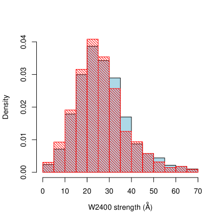
Figure 3: The distribution of the rest-frame equivalent width, $W2400$, is shown for the 75 LQGs with $1.1\leq\bar{z}_{LQG}\leq 1.5$ as the solid histogram (blue online, 1778 quasars). The distribution for the matched control sample (see the text) is shown as the hatched histogram (red online, 1778 quasars). Both are density histograms. Both are for $i\leq 19.1$ and $1.0\leq z\leq 1.8$, with the condition $1.1\leq\bar{z}_{LQG}\leq 1.5$ applied to the LQGs. Other details are as for Fig. 1.

If, having considered the sub-range $1.1\leq\bar{z}_{LQG}\leq 1.5$, we now consider only the remaining $1.5<\bar{z}_{LQG}\leq 1.7$ then there is no perceptible shift at all of the LQG-distribution to higher values of $W2400$. Of course, the number of LQGs and members is then somewhat smaller (36 LQGs, 826 members), but we cautiously conclude that the shift to higher $W2400$ is indeed strongly concentrated in the range $1.1\leq\bar{z}_{LQG}\leq 1.5$.

In summary so far, we find a small but significant shift to higher values of $W2400$ for LQGs with $1.1\leq\bar{z}_{LQG}\leq 1.5$. This result contrasts with that from Harris et al. (2012) and Harris (2011) for a large shift for quasars with $1.1\leq z\leq 1.7$ in the pencil-beam field that intersects the LQGs U1.11, U1.28 and U1.54. However, we do find some indication that the shift that we find here increases to fainter magnitudes. The MMT / Hectospec data used by Harris et al. (2012) and Harris (2011) are for quasars that are typically much fainter than those used here, so it may be that the results can still be reconciled.

Fig. 4 similarly shows the distribution of the rest-frame equivalent width, $W2400$, for the four LQGs U1.11, U1.28 (the CCLQG) and U1.54 (the doubtful LQG), and U1.27 (the Huge-LQG). Their $W2400$ distribution is shown as the solid histogram (blue online), and again the distribution for the corresponding matched control sample is shown as the hatched histogram (red online). The one-sided Mann-Whitney test indicates that there is no significant shift to larger values. From the statistics for the 75 LQGs with $1.1\leq\bar{z}_{LQG}\leq 1.5$ we would, ignoring the different redshift limits arising from the inclusion of U1.54, expect an excess of only 1.6 ultrastrong and 5.8 strong emitters for these four LQGs (166 quasars, 165 with positive $W2400$). Most probably the signal is lost in the noise.

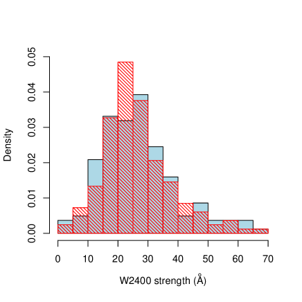
Figure 4: The distribution of the rest-frame equivalent width, $W2400$, is shown for the four LQGs U1.11, U1.28 (the CCLQG), U1.54 (the doubtful LQG) and U1.27 (the Huge-LQG) as the solid histogram (blue online, 165 quasars). The distribution for the matched control sample is shown as the hatched histogram (red online, 165 quasars). Other details are as for Fig. 1.

Note that, very unusually for the DR7QSO catalogue, nine of the 166 spectra for U1.11, U1.27, U1.54 and U1.28 have exposure times of only 900 s. In fact, only U1.11 and U1.28 are affected, with seven of the nine from U1.11 and two from U1.28. Three of the nine are estimated to have s/n $<4$ (two from U1.28 and one from U1.11). The software measurements of $W2400$ place two in the ultrastrong category and one in the strong. Manual measurement suggests that, despite the noise, the software measurements are acceptable.

The members of U1.11, U1.28, U1.54 and U1.27 that have been classified as strong or ultrastrong emitters are listed in Table LABEL:SUS_table. We can briefly compare the classification here with those of Harris (2011) for the small area of the pencil-beam field. The superscripts in the first column of Table LABEL:SUS_table give the corresponding classification from Harris (2011) or, for SDSS J104932.22+050531.7, from Harris (private communication). Note that SDSS J104938.35$+$052932.0 is classified as ultrastrong here and weak in Harris (2011): the software measurement here will be incorrect because of absorption occurring at the position of one of the continuum windows. Two quasars classified as ultrastrong here but strong by Harris are here on the boundary between the ultrastrong and strong classifications. A quasar classified as strong by Harris (2011) but weak by the software measurements, SDSS J104840.34+055912.9 appears on manual checking to be weak.

5 Environments of the ultrastrong UV Fe II emitters

In this section we discuss the environments of the ultrastrong ($W2400\geq 45$ Å) UV Fe II emitters compared with the weak ($W2400<30$ Å) within the 75 LQGs having $1.1\leq\bar{z}_{LQG}\leq 1.5$. We also briefly discuss the particular LQGs U1.11, U1.28, U1.54 and U1.27. If the shift to higher $W2400$ within the LQGs arises from an environmental effect then we might anticipate there will be a density or clustering effect that appears most strongly for the ultrastrong emitters compared with the weak. There is an arbitary element to this approach, of course, because the definitions of ultrastrong, strong and weak emitters involve arbitrary boundaries.

Clowes & Harris (unpublished visualisation) found that the strong and ultrastrong emitters tended to clump with other quasars or with themselves, both within and outside the convex hulls of the three LQGs U1.11, U1.28 and U1.54. (Recall that the deep MMT / Hectospec spectroscopy in the pencil-beam included quasars fainter than the $i\leq 19.1$ limit of the quasars used for the discovery of the LQGs.) Although this visualisation involved no quantification of the clumping, it has guided our thinking that there could be a preferred nearest-neighbour scale for the strongest emitters.

For these reasons, we have investigated the distribution of nearest-neighbour separations for the ultrastrong emitters within the LQGs compared with the distribution for the weak emitters within the LQGs. The nearest neighbours have been determined without regard for the strength of their UV Fe II emission. We consider only the LQGs with $1.1\leq\bar{z}_{LQG}\leq 1.5$, given the earlier result that the shift to higher values of $W2400$ is strongly concentrated in this range.

The distribution of the nearest-neighbour separations (present epoch) for the members of the 75 LQGs with $1.1\leq\bar{z}_{LQG}\leq 1.5$ and for $W2400\geq 45$ Å (i.e. ultrastrong) is shown in Fig. 5 as the solid histogram (blue online), with mean $57.46\pm 1.70$ Mpc. The figure shows also the corresponding distribution for $W2400<30$ Å (i.e. weak) as the hatched histogram (red online), with mean $59.65\pm 0.63$ Mpc. Both are density histograms. Both are for $i\leq 19.1$ and $1.0\leq z\leq 1.8$. Although drawn from the same LQGs, the two histograms appear different, with that for $W2400\geq 45$ Å indicating preferred values of the nearest-neighbour separation predominantly in the range $\sim$ 25–50 Mpc (present epoch) — note the consecutive bins where the histogram for $W2400\geq 45$ Å exceeds the histogram for $W2400<30$ Å. A Mann-Whitney test is inappropriate here because the LQG-finding algorithm restricts separations to $\leq$ 100 Mpc, but a one-sided Kolmogorov-Smirnov test indicates that the CDF (cumulative distribution function) of the $W2400\geq 45$ Å distribution is greater than the CDF of the $W2400<30$ Å distribution, with p-value $=0.0255$, which is marginally significant.

Given the arbitrary boundaries for the definitions of ultrastrong, strong and weak emitters we note that a post-hoc adjustment from $W2400\geq 45$ Å to $W2400\geq 44$ Å gives the histograms shown in Fig. 6, with means $57.40\pm 1.60$, $59.65\pm 0.63$ Mpc, and the Kolmogorov-Smirnov test gives a p-value $=0.0197$. The preferred nearest-neighbour separation appears then to be predominantly in the range $\sim$ 30–50 Mpc.

Figure 5: The distribution of the nearest-neighbour separations (present epoch) for the members of the 75 LQGs with $1.1\leq\bar{z}_{LQG}\leq 1.5$ and for $W2400\geq 45$ Å (i.e. ultrastrong) is shown as the solid histogram (blue online, 143 quasars), with mean $57.46\pm 1.70$ Mpc. The distribution for the members of the LQGs with $W2400<30$ Å is shown as the hatched histogram (red online, 1152 quasars), with mean $59.65\pm 0.63$ Mpc. Both are density histograms. Both are for $i\leq 19.1$ and $1.0\leq z\leq 1.8$. The bin size is 5 Mpc. Note the apparent preference of the $W2400\geq 45$ Å quasars for separations in the range 25–50 Mpc. Note that the LQG-finding algorithm restricts separations to $\leq 100$ Mpc.

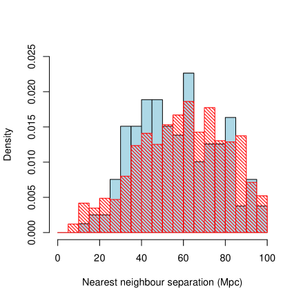
Figure 6: The distribution of the nearest-neighbour separations (present epoch) for the members of the 75 LQGs with $1.1\leq\bar{z}_{LQG}\leq 1.5$ and for $W2400\geq 44$ Å (post-hoc adjustment) is shown as the solid histogram (blue online, 160 quasars), with mean $57.40\pm 1.60$ Mpc. The distribution for the members of the LQGs with $W2400<30$ Å is shown as the hatched histogram (red online, 1152 quasars), with mean $59.65\pm 0.63$ Mpc. Both are density histograms. Both are for $i\leq 19.1$ and $1.0\leq z\leq 1.8$. The bin size is 5 Mpc. Note the apparent preference of the $W2400\geq 44$ Å quasars for separations in the range 30–50 Mpc. Note that the LQG-finding algorithm restricts separations to $\leq 100$ Mpc.

Although we find evidence for a preferred nearest-neighbour scale for the ultrastrong-emitting quasars in LQGs we find no evidence for a preferred scale in the quasars that are not members of LQGs (mean nearest-neighbour separation $\sim$ 78 Mpc), across a comparable range of redshifts. Thus the preferred nearest-neighbour scale of $\sim$ 30–50 Mpc for the $W2400\geq 45$ Å (more precisely, $W2400\geq 44$ Å) emitters seems to be peculiar to the LQG environment. Presumably, it is related to the shift to higher $W2400$ values within the LQGs.

We have similarly used the visualisation software to look at the environments of the strongest emitters from the entire memberships of the same three LQGs from Harris et al. (2012) and Harris (2011), U1.11, U1.28 and U1.54, together with U1.27. Given the above result on the nearest-neighbour separations we concentrate on the quasars with $W2400\geq 44$ Å rather than simply $W2400\geq 45$ Å. To simplify the discussion we introduce an ultrastrong-plus category as those with $W2400\geq 44$ Å (while still retaining “ultrastrong” as those with $W2400\geq 45$ Å). The findings are similar to those previously, but not always so clear, perhaps because of the brighter limiting magnitude. For example, with U1.54, the doubtful LQG, only two of the five ultrastrong-plus emitters appear to be closely associated with other quasars, and only one of these is in a dense region. In contrast, with U1.11, three of four ultrastrong-plus emitters do seem to be associated with other quasars and denser regions. With U1.28, two of four ultrastrong-plus emitters appear to be close to other quasars, but with neither being in particularly dense regions. With U1.27 (the Huge-LQG), six of the seven ultrastrong-plus emitters form three pairs (separations 52, 81, 105 Mpc), within the total membership of 73. One pairing is actually part of a close triplet with another quasar in a generally dense region, and another pairing is part of a looser triplet in a less dense region. The third pairing has one quasar in a dense region and the other detached from it. The seventh ultrastrong-plus quasar is close to another quasar in a less dense region. A visualisation of the location of these seven ultrastrong-plus emitters within U1.27 is shown in Fig. 7.

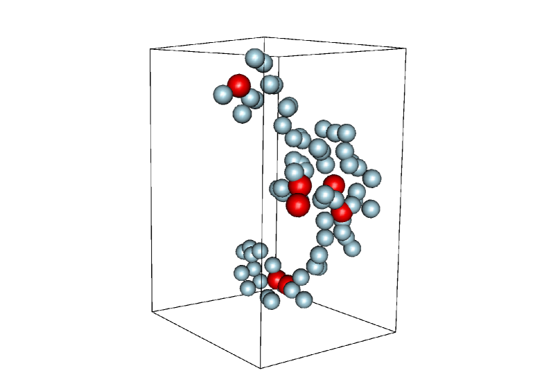
Figure 7: Visualisation of the location of the seven ultrastrong-plus emitters ($W2400\geq 44$ Å) within U1.27, the Huge-LQG. The LQG has 73 members. Sixty-six of the members are represented by spheres of radius that corresponds to 33 Mpc (present epoch, blue online). The seven ultrastrong-plus quasars are represented by slightly larger spheres of radius that corresponds to 40 Mpc (red online). The long dimension of the surrounding box corresponds to approximately 1000 Mpc.

6 Discussion and conclusions

We have compared the distribution of the $W2400$ equivalent width of UV Fe II emitting quasars in the dense environments of 111 LQGs having $1.1\leq\bar{z}_{LQG}\leq 1.7$ with the distribution for quasars that are not in LQGs. We find a marginally significant shift (p-value $=0.0226$, shift $=0.62$ Å) of the $W2400$ distribution to higher values for quasars within LQGs. The shift appears to be a stronger effect at fainter magnitudes $18.0\leq i\leq 19.1$ (p-value $=0.0064$, shift $=0.84$ Å).

However, the shift to higher $W2400$ appears to be strongly concentrated in the 75 LQGs having $1.1\leq\bar{z}_{LQG}\leq 1.5$ (p-value $=0.0042$, shift $=0.97$ Å), and again it appears to be a stronger effect at fainter magnitudes $18.0\leq i\leq 19.1$ (p-value $=0.00054$, shift $=1.31$ Å).

We have investigated the distribution of nearest-neighbour separations for the ultrastrong emitters within the 75 LQGs having $1.1\leq\bar{z}_{LQG}\leq 1.5$ compared with the distribution for the weak emitters. The nearest neighbours were determined without regard for the strength of their UV Fe II emission. We found a marginally significant result (p-value $=0.0255$) that the CDF of the ultrastrong ($W2400\geq 45$ Å) distribution is greater than the CDF of the weak ($W2400<30$ Å) distribution. There appears to be a preferred nearest-neighbour separation predominantly in the range $\sim$ 25–50 Mpc. We found that a post-hoc adjustment from ultrastrong $W2400\geq 45$ Å to “ultrastrong-plus” $W2400\geq 44$ Å gives improved significance (p-value $=0.0197$), and a preferred nearest-neighbour separation that then appears to be predominantly in the range $\sim$ 30–50 Mpc.

Our finding of a shift towards higher values of $W2400$ for quasars within LQGs is compatible with the result from Harris et al. (2012) and Harris (2011) of a shift for a deep pencil-beam field that intersects the three LQGs U1.11, U1.28 and U1.54 (the doubtful LQG). Our shift seems smaller, but we do find an indication that the shift will increase to fainter magnitudes. The MMT / Hectospec data used by Harris et al. (2012) and Harris (2011) are for quasars that are typically much fainter than those used here, so it may be that the size of the shifts can still be reconciled. However, there is an inevitable difficulty in constructing a matching control sample for the faint MMT / Hectospec sample, so possibly the attempted allowance for the differences has not been wholly successful and the size of the shift there then appears larger than it should be. We find that the shift is strongly concentrated in the range $1.1\leq\bar{z}_{LQG}\leq 1.5$. U1.54 is excluded from our data by this condition of course, but fundamentally it is excluded because it fails our CHMS-significance criterion.

Clowes & Harris (unpublished visualisation) noted, for the pencil-beam field within U1.11, U1.28 and U1.54, a tendency for strong / ultrastrong emitters to clump with other quasars or with themselves. With the data for the 75 LQGs having $1.1\leq\bar{z}_{LQG}\leq 1.5$ in this paper we find evidence that ultrastrong-plus emitters — those with $W2400\geq 44$ Å — have a preferred nearest-neighbour scale of $\sim$ 30–50 Mpc. This result supports, and makes quantitative, the result from the visualisation. However, no such preferred scale is seen for ultrastrong-plus emitters that are not in LQGs.

Our visualisation of the ultrastrong-plus emitters across U1.11, U1.28 and U1.54 in their entireties, together with U1.27, is generally consistent with the deeper pencil-beam visualisation but not so clear. A striking result, however, is from U1.27, the Huge-LQG, for which six of the seven ultrastrong-plus emitters, from amongst the total of 73 LQG members, form three pairings.

We have thus found two effects of the dense LQG environment on the ultraviolet Fe II emission of the member quasars. Firstly, there is a general shift to higher $W2400$, compared with non-members for $1.1\leq\bar{z}_{LQG}\leq 1.5$. The shift appears to be stronger for fainter magnitudes. This redshift dependence, $\bar{z}_{LQG}\leq 1.5$, suggests an evolutionary effect. Secondly, we find evidence for a preferred nearest-neighbour separation of $\sim$ 30–50 Mpc for the ultrastrong ($W2400\geq 45$ Å) or, more precisely, ultrastrong-plus ($W2400\geq 44$ Å) emitters compared with the weak ($W2400<30$) emitters within these LQGs. This preferred separation suggests a clustering or dynamical effect. Of course, there may be further subtleties present in the dependences on redshift, magnitude and density than we have seen, but a still larger sample with which to disentangle them is not currently feasible. It may be, however, that a different approach on the existing data, such as fitting templates to the Fe II, could restore some information that might presently be lost to uncertainties in measuring $W2400$.

The possibilities for increasing the strength of the Fe II emission appear to be iron abundance, Ly-$\alpha$ fluorescence, and microturbulence. Probably all of these operate. The dense environment of the LQGs and an increased rate of interactions and mergers between galaxies may have led to an increased rate of star formation and an enhanced abundance of iron in the nuclei of galaxies. Similarly the dense environment of the LQGs may have led to more active blackholes and increased Ly-$\alpha$ emission. The preferred nearest-neighbour separation for the stronger emitters would appear to suggest a dynamical component, such as microturbulence.

7 Acknowledgments

The anonymous referee is thanked for helpful comments and suggestions.

LEC received partial support from the Center of Excellence in Astrophysics and Associated Technologies (PFB 06), and from a CONICYT Anillo project (ACT 1122).

SR is in receipt of a CONICYT PhD studentship.

This research has used the SDSS DR7QSO catalogue (Schneider et al., 2010).

Funding for the SDSS and SDSS-II has been provided by the Alfred P. Sloan Foundation, the Participating Institutions, the National Science Foundation, the U.S. Department of Energy, the National Aeronautics and Space Administration, the Japanese Monbukagakusho, the Max Planck Society, and the Higher Education Funding Council for England. The SDSS Web Site is http://www.sdss.org/.

The SDSS is managed by the Astrophysical Research Consortium for the Participating Institutions. The Participating Institutions are the American Museum of Natural History, Astrophysical Institute Potsdam, University of Basel, University of Cambridge, Case Western Reserve University, University of Chicago, Drexel University, Fermilab, the Institute for Advanced Study, the Japan Participation Group, Johns Hopkins University, the Joint Institute for Nuclear Astrophysics, the Kavli Institute for Particle Astrophysics and Cosmology, the Korean Scientist Group, the Chinese Academy of Sciences (LAMOST), Los Alamos National Laboratory, the Max-Planck-Institute for Astronomy (MPIA), the Max-Planck-Institute for Astrophysics (MPA), New Mexico State University, Ohio State University, University of Pittsburgh, University of Portsmouth, Princeton University, the United States Naval Observatory, and the University of Washington.

References

- Baldwin et al. (2004) Baldwin J.A., Ferland G.J., Korista K.T., Hamann F., LaCluyzé A., 2004, ApJ, 615, 610
- Bruhweiler & Verner (2008) Bruhweiler F., Verner E., 2008, ApJ, 675, 83
- Clowes & Campusano (1991) Clowes R.G., Campusano L.E., 1991, MNRAS, 249, 218
- Clowes et al. (2012) Clowes R.G., Campusano L.E., Graham M.J., Söchting I.K., 2012, MNRAS, 419, 556
- Clowes et al. (2013) Clowes R.G., Harris K.A., Raghunathan S., Campusano L.E., Söchting I.K., Graham M.J., 2013, MNRAS, 429, 2910
- Collin-Souffrin & Lasota (1988) Collin-Souffrin S., Lasota J.-P., 1988, PASP, 100, 1041
- (7) Graham M.J., Clowes R.G., Campusano L.E., 1996, MNRAS, 279, 1349
- Harris (2011) Harris K.A., PhD thesis, Univ. of Central Lancashire (astro-ph/1201.5746)
- Harris et al. (2012) Harris K.A., Clowes R.G., Williger G.M., Haberzettl L.G., Campusano L.E., 2012, in Boissier S., de Laverny P., Nardetto N., Samadi R., Valls-Gabaud D., Wozniak H., eds, SF2A-2012: Proceedings of the Annual meeting of the French Society of Astronomy and Astrophysics, p. 469
- Meusinger et al. (2012) Meusinger H., Schalldach P., Scholz R.-D., in der Au A., Newholm M., de Hoon A., Kaminsky B., 2012, A&A, 541, A77
- Newman et al. (1998) Newman P.R., Clowes R.G., Campusano L.E., Graham M.J., 1998, in Müller V., Gottlöber S., Mücket J.P., Wambsganss J., eds, Large Scale Structure: Tracks and Traces. World Scientific, Singapore, p. 133
- Newman (1999) Newman P.R., 1999, PhD thesis, Univ. of Central Lancashire
- Penston (1987) Penston M.V., 1987, MNRAS, 229, 1P
- Richards et al. (2006) Richards G.T. et al., 2006, AJ, 131, 2766
- Ruff et al. (2012) Ruff A.J., Floyd D.J.E., Webster R.L., Korista K.T., Landt H., 2012, ApJ, 754:18
- Schneider et al. (2010) Schneider D.P. et al., 2010, AJ, 139, 2360
- Shen et al. (2011) Shen Y. et al., 2011, ApJS, 194:45
- Sigut & Pradhan (1998) Sigut T.A.A., Pradhan A.K., 1998, ApJ, 499, L139
- Sigut & Pradhan (2003) Sigut T.A.A., Pradhan A.K., 2003, ApJS, 145, 15
- Vanden Berk et al. (2005) Vanden Berk D.E., et al., 2005, AJ, 129, 2047
- Weymann et al. (1991) Weymann R.J., Morris S.L., Foltz C.B., Hewett P.C., 1991, ApJ, 373, 23
- (22) Wills B.J., Netzer H., Wills D., 1985, ApJ, 288, 94
- Zhang (2011) Zhang X.-G., 2011, ApJ, 741, 104