About presentations of braid groups and their generalizations

Abstract.

In the paper we give a survey of rather new notions and results which generalize classical ones in the theory of braids. Among such notions are various inverse monoids of partial braids. We also observe presentations different from standard Artin presentation for generalizations of braids. Namely, we consider presentations with small number of generators, Sergiescu graph-presentations and Birman-Ko-Lee presentation. The work of V. V. Chaynikov on the word and conjugacy problems for the singular braid monoid in Birman-Ko-Lee generators is described as well.

1. Introduction

The purpose of this paper is to give a survey on some recent notions and results concerning generalizations of the braids.

Classical braid groups $Br_{n}$ can be defined in several ways. Either as a set of isotopy classes of system of $n$ curves in a three-dimensional space (what is the same as the fundamental group of the configuration space of $n$ points on a plane) or as the mapping class group of a disc with $n$ points deleted $D_{n}$ with its boundary fixed, what is equivalent to the subgroup of the braid automorphisms of the automorphism group of a free group $\operatorname{Aut}F_{n}$. For the exact definitions we make a reference here to a monograph on braid, for example the book of C. Kassel and V. Turaev [46] or to the previous surveys of the author [79, 81, 84].

The pure braid group $P_{n}$ is defined as the kernel of the canonical epimorphism $\tau_{n}$ from braids to the symmetric group $\Sigma_{n}$:

$$1\rightarrow P_{n}\rightarrow Br_{n}\buildrel\tau_{n}\over{\longrightarrow}\Sigma_{n}\rightarrow 1.$$

We fix the canonical Artin presentation [2] of the braid group $Br_{n}$. It has generators $\sigma_{i}$, $i=1,...,n-1$ and two types of relations:

(1.1) $$\begin{cases}\sigma_{i}\sigma_{j}&=\sigma_{j}\,\sigma_{i},\ \ \text{if}\ \ |i-j|>1,\\ \sigma_{i}\sigma_{i+1}\sigma_{i}&=\sigma_{i+1}\sigma_{i}\sigma_{i+1}.\end{cases}$$

The generators $\sigma_{i}$ correspond to the following automorphisms of $F_{n}$:

(1.2) $$\begin{cases}x_{i}&\mapsto x_{i+1},\\ x_{i+1}&\mapsto x_{i+1}^{-1}x_{i}x_{i+1},\\ x_{j}&\mapsto x_{j},j\not=i,i+1.\end{cases}$$

Of course, there exist other presentations of the braid group. Let

(1.3) $$\sigma=\sigma_{1}\sigma_{2}\dots\sigma_{n-1},$$

then the group $Br_{n}$ is generated by $\sigma_{1}$ and $\sigma$ because

(1.4) $$\sigma_{i+1}=\sigma^{i}\sigma_{1}\sigma^{-i},\quad i=1,\dots n-2.$$

The relations for the generators $\sigma_{1}$ and $\sigma$ are the following

(1.5) $$\begin{cases}\sigma_{1}\sigma^{i}\sigma_{1}\sigma^{-i}&=\sigma^{i}\sigma_{1}\sigma^{-i}\sigma_{1}\ \ \text{for}\ \ 2\leq i\leq{n/2},\\ \sigma^{n}&=(\sigma\sigma_{1})^{n-1}.\end{cases}$$

The presentation (1.5) was given by Artin in the initial paper [2]. This presentation was also mentioned in the books by F. Klein [48] and by H. S. M. Coxeter and W. O. J. Moser [23].

V. Ya. Lin in [55] gives a slightly different form of this presentation. Let $\beta\in Br_{n}$ be defined by the formula

$$\beta=\sigma\sigma_{1}.$$

Then there is the presentation of the group $Br_{n}$ with generators $\sigma_{1}$ and $\beta$ and relations:

$$\begin{cases}\beta\sigma^{i-1}\beta&=\sigma^{i}\beta\sigma^{-i-1}\beta\sigma^{i}\ \ \text{for}\ \ 2\leq i\leq{n/2},\\ \sigma^{n}&=\beta^{n-1}.\end{cases}$$

This presentation is called special in [55].

An interesting series of presentations was given by V. Sergiescu [72]. For every planar graph he constructed a presentation of the group $Br_{n}$, where $n$ is the number of vertices of the graph, with generators corresponding to edges and relations reflecting the geometry of the graph. To each edge $e$ of the graph he associates the braid $\beta_{e}$ which is a clockwise half-twist along $e$ (see Figure 1.1). Artin’s classical presentation (1.1) in this context corresponds to the graph consisting of the interval from 1 to $n$ with the natural numbers (from 1 to $n$) as vertices and with segments between them as edges.

Figure 1.1. Edges and geometric braids.

To be precise let $\Gamma$ be a planar graph. We call it normal if $\Gamma$ is connected, and it has no loops or intersections. Let $S(\Gamma)$ be the set of vertices of $\Gamma$. If $\Gamma$ is not a tree then we define next what is a pseudocycle on it. The bounded part of the complement of $\Gamma$ in the plane is the disjoint union of a finite number of open disks $D_{1},\dots,D_{m}$, $m>1$. The boundary of $D_{j}$ on the plane is a subgraph $\Gamma(D_{j})$ of $\Gamma$. We choose a point $O$ in the interior of $D_{j}$, and an edge $\sigma$ of $\Gamma(D_{j})$ with vertices $v_{1},v_{2}$. We suppose that the triangle $Ov_{1}v_{2}$ is oriented anticlockwise. We denote $\sigma$ by $\sigma(e_{1})$. We define the pseudocycle associated to $D_{j}$ to be the sequence of edges $\sigma(e_{1})\dots\sigma(e_{p})$ such that:

-if the vertex $v_{j+1}$ is not uni-valent, then $\sigma(e_{j+1})$ is the first edge on the left of $\sigma(e_{j})$ (we consider $\sigma(e_{j})$ going from $v_{j}$ to $v_{j+1}$) and the vertex $v_{j+2}$ is the other vertex adjacent to $\sigma(e_{j+1})$;

-if the vertex $v_{j+1}$ is uni-valent, then $\sigma(e_{j+1})=\sigma(e_{j})$ and $v_{j+2}=v_{j}$.

-the vertex $v_{p+1}$ is the vertex $v_{1}$.

Let $\gamma=\sigma(e_{1})\dots\sigma(e_{p})$ be a pseudocycle of $\Gamma$. Let $i=1,\dots,p$. If $\sigma(e_{i})=\sigma(e_{j})$ for some $j\not=i$, then we say that

• $\sigma(e_{i})$ is the start edge of a reverse if $j=i+1$ (we set $e_{p+1}=e_{1}$),

• $\sigma(e_{i})$ is the end edge of a reverse if $j=i-1$ (we set $e_{0}=e_{p}$).

In the following we set $\sigma_{1}\dots\sigma_{p}$ for the pseudocycle $\sigma(e_{1})\dots\sigma(e_{p})$.

Theorem 1.1.

(V. Sergiescu [72]) Let $\Gamma$ be a normal planar graph with $n$ vertices. The braid group $Br_{n}$ admits a presentation $\langle X_{\Gamma}\,|\,R_{\Gamma}\rangle$, where $X_{\Gamma}=\{\sigma\;|\;\sigma\;\mbox{is an edge of }\;\Gamma\}$ and $R_{\Gamma}$ is the set of following relations:

• Disjointedness relations (DR): if $\sigma_{i}$ and $\sigma_{j}$ are disjoint, then $\sigma_{i}\sigma_{j}=\sigma_{j}\sigma_{i}$;

• Adjacency relations (AR): if $\sigma_{i},\sigma_{j}$ have a common vertex, then $\sigma_{i}\sigma_{j}\sigma_{i}$ $=\sigma_{j}\sigma_{i}\sigma_{j}$;

• Nodal relations (NR): if $\{\sigma_{1},\sigma_{2},\sigma_{3}\}$ have only one common vertex and they are clockwise oriented (Figure 1.2), then

  $$\sigma_{1}\sigma_{2}\sigma_{3}\sigma_{1}=\sigma_{2}\sigma_{3}\sigma_{1}\sigma_{2}\,;$$

• Pseudocycle relations (PR): if $\sigma_{1}\dots\sigma_{m}$ is a pseudocycle and $\sigma_{1}$ is not the start edge or $\sigma_{m}$ the end edge of a reverse (Figure 1.3), then

  $$\sigma_{1}\sigma_{2}\cdots\sigma_{m-1}=\sigma_{2}\sigma_{3}\cdots\sigma_{m}\,.$$

Figure 1.2. Nodal relation.

Figure 1.3. Pseudocycle relation; on the left $\sigma_{1}\sigma_{2}\cdots\sigma_{m-1}=\sigma_{2}\cdots\sigma_{m}=\dots=\sigma_{m}\cdots\sigma_{m-2}$. On the right $\sigma_{1}\sigma_{2}\sigma_{3}^{2}=\sigma_{2}\sigma_{3}^{2}\sigma_{4}=\sigma_{3}^{2}\sigma_{4}\sigma_{1}$ and $\sigma_{3}\sigma_{4}\sigma_{1}\sigma_{2}=\sigma_{4}\sigma_{1}\sigma_{2}\sigma_{3}$.

Remark 1.1.

Theorem 1.1 is true for infinite graphs. Let $\Gamma$ be the direct limit of its finite subgraphs $\Gamma_{i}$, then the braid group $Br_{\Gamma}$ is the direct limit of the subgroups $Br_{\Gamma_{i}}$.

The graph presentation of Sergiescu underlines the geometric character of braids, its connection with configuration spaces. In this survey we confirm this proposing a thesis: for every generalization of braids of geometric character there exists a graph presentation.

Birman, Ko and Lee [14] introduced the presentation with the generators $a_{ts}$ with $1\leq s<t\leq n$ and relations

$$\begin{cases}a_{ts}a_{rq}&=a_{rq}a_{ts}\ \ {\rm for}\ \ (t-r)(t-q)(s-r)(s-q)>0,\\ a_{ts}a_{sr}&=a_{tr}a_{ts}=a_{sr}a_{tr}\ \ {\rm for}\ \ 1\leq r<s<t\leq n.\end{cases}$$

The generators $a_{ts}$ are expressed by the canonical generators $\sigma_{i}$ in the following form:

$$a_{ts}=(\sigma_{t-1}\sigma_{t-2}\cdots\sigma_{s+1})\sigma_{s}(\sigma^{-1}_{s+1}\cdots\sigma^{-1}_{t-2}\sigma^{-1}_{t-1})\ \ {\rm for}\ \ 1\leq s<t\leq n.$$

Geometrically the generators $a_{s,t}$ are depicted in Figure 1.4. These generators are very natural and for this presentation Birman, Ko and Lee proposed an algorithm which solves the word problem with the speed $\mathcal{O}(m^{2}n)$ while Garside algorithm [37] improved by W. Turston has a speed $\mathcal{O}(m^{2}n\log n)$, where $m$ is the length of a word and $n$ is the number of strands (see [30], Corollary 9.5.3). The question of generalization of this presentation for other types of braids was raised in [14].

Figure 1.4.

In Section 2 we describe generalizations of braids that will be involved. In Section 3 we give the presentations with few generators, in Section 4 we study graph-presentations in the sense of V. Sergiescu and in Section 5 we give the Birman-Ko-Lee presentation for the singular braid monoid. In Section 6 we describe the work of V. V. Chaynikov [20] on the word and conjugacy problems for the singular braid monoid in Birman-Ko-Lee generators. In Sections 7 – 9 we study inverse monoids of partial braids.

The author is thankful to the organizers of Knots in Poland III Józef Przytycki and Pawel Trazcyk for the excellent conference.

2. Generalizations of Braids

It is interesting to obtain the analogues of the presentations mentioned in the Introduction for various generalizations of braids [3], [13], [16], [27], [35], [80].

2.1. Artin-Brieskorn braid groups

Let $I$ be a set and $M=(m_{i,j})$, is a matrix, $m_{i,j}\ \in\mathbb{N}^{+}\cup\{\infty\}$, $i,j\in I$ with the following conditions: $m_{i,i}=1$ and $m_{i,j}>1$ for $i\not=j$. J. Tits in [74] defines the Coxeter group of type $M$ as a group with generators $w_{i}$, $i\in I$ and relations

$$(w_{i}w_{j})^{m_{i,j}}=e,\ i,j\in I.$$

The corresponding braid groups, which are called Artin-Tits groups have the elements $s_{i}$, $i\in I$ as the generators and the following set of defining relations:

$$\operatorname{prod}(m_{i,j};s_{i},s_{j})=\operatorname{prod}(m_{j,i};s_{j},s_{i}),$$

where $\operatorname{prod}(m;x,y)$ denotes the product $xyxy...$ ($m$ factors).

Classification of irreducible finite Coxeter groups is well known (see for example Theorem 1, Chapter VI, §4 of [15]). It consists of the three infinite series: $A$, $B$ and $D$ as well as the exceptional groups $E_{6},E_{7},E_{8},F_{4}$, $G_{2}$, $H_{3}$, $H_{4}$ and $I_{2}(p).$

Let $N$ be a finite set of cardinality $n$, say $N=\{v_{1},\dots,v_{n}\}$. Let us equip elements of $N$ with the signs, i.e. let $SN=\{\delta_{1}v_{1},\dots,\delta_{n}v_{n}\}$, where $\delta_{i}=\pm 1$. The Coxeter group $W(B_{n})$ of type $B$ can be interpreted as a group of signed permutations of the set $SN$:

(2.1) $$W(B_{n})=\{\sigma-\text{ bijection \ of }SN:(-x)\sigma=-(x)\sigma\text{ for}\ x\in SN\}.$$

The generalized braid group (or Artin–Brieskorn group) $Br(W)$ of $W$ [16], [27] correspond to the case of finite Coxeter group $W$. The classical braids on $k$ strings $Br_{k}$ are obtained by this construction if $W$ is the symmetric group on $k$ symbols. In this case $m_{i,i+1}=3$, and $m_{i,j}=2$ if $j\neq i,i+1$.

The braid group of type $B_{n}$ has the canonical presentation with generators $\sigma_{i}$, $i=1,\dots,n-1$ and $\tau$, and relations:

(2.2) $$\begin{cases}\sigma_{i}\sigma_{j}&=\sigma_{j}\sigma_{i},\ \ \text{if}\ \ |i-j|>1,\\ \sigma_{i}\sigma_{i+1}\sigma_{i}&=\sigma_{i+1}\sigma_{i}\sigma_{i+1},\\ \tau\sigma_{i}&=\sigma_{i}\tau,\ \ \text{if}\ \ i\geq 2,\\ \tau\sigma_{1}\tau\sigma_{1}&=\sigma_{1}\tau\sigma_{1}\tau.\\ \end{cases}$$

This group can be identified with the fundamental group of the configuration space of distinct points on the plane with one point deleted [52], [76], what is the same as the braid group on $n$ strands on the annulus, $Br_{n}(Ann)$. A geometric interpretation of generators $\tau,\sigma_{1},\dots,\sigma_{n-1}$ is given in Figure 2.1.

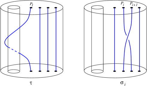
Figure 2.1. Geometric interpretation of generators $\tau,\sigma_{1},\dots,\sigma_{n-1}$ of $Br_{n}(Ann)$.

The braid groups of the type $D_{n}$ has the canonical presentation with generators $\sigma_{i}$ and $\rho$, and relations:

(2.3) $$\begin{cases}\sigma_{i}\sigma_{j}&=\sigma_{j}\sigma_{i}\ \ \text{if}\ \ |i-j|>1,\\ \sigma_{i}\sigma_{i+1}\sigma_{i}&=\sigma_{i+1}\sigma_{i}\sigma_{i+1},\\ \rho\sigma_{i}&=\sigma_{i}\rho\ \ \text{if}\ \ i=1,3,\dots,n-1,\\ \rho\sigma_{2}\rho&=\sigma_{2}\rho\sigma_{2}.\\ \end{cases}$$

Let V be a complex finite dimensional vector space. A pseudo-reflection of $GL(V)$ is a non trivial element $s$ of $GL(V$) which acts trivially on a hyperplane, called the reflecting hyperplane of $s$. Suppose that $W$ is a finite subgroup of $GL(V)$ generated by pseudo-reflections; the corresponding braid groups were studied by M. Broué, G. Malle and R. Rouquier [18] and also by D. Bessis and J. Michel [12]. As in the classical case these groups can be defined as fundamental groups of complement in $V$ of the reflecting hyperplanes. The following classical conjecture generalizes the case of braid groups:

The universal cover of complement in $V$ of the reflecting hyperplane is contractible.

(See for example the book by Orlik and Terao [63], p. 163 & p. 259)

This conjecture was proved by David Bessis [11]. It means that these groups has naturally defined finite dimensional manifold as $K(\pi,1)$-spaces.

2.2. Braid groups on surfaces

Let $\Sigma$ be surface. The $n$th braid group of $\Sigma$ can be defined as the fundamental group of configuration space of $n$ points on $\Sigma$. Let $\Sigma$ be a sphere. The corresponding braid group $Br_{n}(S^{2})$ has simple geometric interpretation as a group of isotopy classes of braids lying in a layer between two concentric spheres. It has the presentation with generators $\delta_{i}$, $i=1,...,n-1$, which satisfy the braid relations (1.1) and the following sphere relation:

(2.4) $$\delta_{1}\delta_{2}\dots\delta_{n-2}\delta_{n-1}^{2}\delta_{n-2}\dots\delta_{2}\delta_{1}=1.$$

This presentation was found by O. Zariski [88] in 1936 and then rediscovered by E. Fadell and J. Van Buskirk [32] in 1961.

Presentations of braid groups on all closed surfaces were obtained by G. P. Scott [71] and others.

2.3. Braid-permutation group

Let $BP_{n}$ be the subgroup of $\operatorname{Aut}F_{n}$, generated by both sets of the automorphisms $\sigma_{i}$ of (1.2) and $\xi_{i}$ of the following form:

(2.5) $$\begin{cases}x_{i}&\mapsto x_{i+1},\\ x_{i+1}&\mapsto x_{i},\\ x_{j}&\mapsto x_{j},j\not=i,i+1,\end{cases}$$

This is the $n$th braid-permutation group introduced by R. Fenn, R. Rimányi and C. Rourke [35] who gave a presentation of this group: it consists of the set of generators: $\{\xi_{i},\sigma_{i},\ \ i=1,2,...,n-1\}$ such that $\sigma_{i}$ satisfy the braid relations, $\xi_{i}$ satisfy the symmetric group relations and both of them the satisfy the following mixed relations:

(2.6) $$\begin{cases}\sigma_{i}\xi_{j}&=\xi_{j}\sigma_{i},\ \text{if}\ |i-j|>1,\\ \xi_{i}\xi_{i+1}\sigma_{i}&=\sigma_{i+1}\xi_{i}\xi_{i+1},\\ \sigma_{i}\sigma_{i+1}\xi_{i}&=\xi_{i+1}\sigma_{i}\sigma_{i+1}.\end{cases}$$

The mixed relations for the braid-permutation group

R. Fenn, R. Rimányi and C. Rourke gave a geometric interpretation of $BP_{n}$ as a group of welded braids.

This group was also studied by A. G. Savushkina [70] under the name of group of conjugating automorphisms and notation ${\mathbf{C}}_{n}$.

Braid-permutation group has an interesting geometric interpretation as a motion group. This group was introduced in the PhD thesis of David Dahm, a student of Ralph Fox. It appeared in literature in the paper of Deborah Goldsmith [41] and then studied by various authors, see, [44], for instance. This is an analogue of the interpretation of the classical braid group as a mapping class group of a punctured disc. Instead of $n$ points in a disc we consider $n$ unlinked unknotted circles in a 3-ball. The fundamental group of the complement of $n$ circles is also the free group $F_{n}$. Interchanging of two neighbour points in the case of the braid group corresponds to an automorphism (1.2) of the free group. In the case of circles this automorphism corresponds to a motion of two neighbour circles when one of the circles is passing inside another one. Simple interchange of two neighbour circles corresponds to the automorphism (2.5).

Another motivation for studing braid-permutation groups is given by the pure braid-permutation group $P\varSigma_{n}$, the kernel of the canonical epimorphism $BP_{n}\to\Sigma_{n}$. In the context of the motion group it is called as the group of loops, but it has even a longer history and is connected with classical works of J. Nielsen [62] and W. Magnus [56] (see also [57]), as follows. Let us denote the kernel of the natural map

$$Aut(F_{n})\to GL(n,\mathbb{Z})$$

by $IA_{n}$. These groups are similar to the Torelli subgroups of the mapping class groups. Nielsen, and Magnus gave automorphisms which generate $IA_{n}$ as a group. These automorphisms are named as follows:

• $\chi_{k,i}$ for $i\neq k$ with $1\leq i,k\leq n$, and

• $\theta(k;[s,t])$ for $k,s,t$ distinct integers with $1\leq k,s,t\leq n$ and $s<t$.

The definition of the map $\chi_{k,i}$ is given by the formula

$$\chi_{k,i}(x_{j})=\begin{cases}x_{j}&\text{if $k\neq j$,}\\ (x_{i}^{-1})(x_{k})(x_{i})&\text{if $k=j$.}\end{cases}$$

The map $\theta(k;[s,t])$ is defined by the formula

$$\theta(k;[s,t])(x_{j})=\begin{cases}x_{j}&\text{if $k\neq j$,}\\ (x_{k})\cdot([x_{s},x_{t}])&\text{if $k=j$.}\end{cases}$$

for which the commutator is given by $[a,b]=a^{-1}\cdot b^{-1}\cdot a\cdot b$.

The group $IA_{2}$ is isomorphic to the group of inner automorphisms ${\rm Inn}(F_{2})$, which is isomorphic to the free group $F_{2}$. The group $IA_{3}$ is not finitely presented [51].

Consider the subgroup of $IA_{n}$ generated by the $\chi_{k,i}$, the group of basis conjugating automorphisms of a free group. This is exactly $P\varSigma_{n}$. McCool gave a presentation for it [59].

The cohomology of $P\varSigma_{n}$ was computed by C. Jensen, J. McCammond, and J. Meier [44]. N. Kawazumi [47], T. Sakasai [68], T. Satoh [69] and A. Pettet [66] have given related cohomological information for $IA_{n}$. The integral cohomology of the natural direct limit of the groups $Aut(F_{n})$ is given in work of S. Galatius [36].

Theorem 2.1.

(A. G. Savushkina [70]) The group $\mathrm{BP}_{n}$ is the semi-direct product of the symmetric group on $n$-letters $\Sigma_{n}$ and the group $P\varSigma_{n}$ with a split extension

$$\begin{CD}1@>{}>{}>P\varSigma_{n}@>{}>{}>\mathrm{BP}_{n}@>{}>{}>\Sigma_{n}@>{}>{}>1.\end{CD}$$

The Lie algebra structure obtained from the descending central series of the group $P\varSigma_{n}$ was studied by F. R. Cohen, J.  Pakianathan, V. V. Vershinin and J. Wu [21] and by B. Berceanu and S. Papadima [9]. Certain subgroups of $P\varSigma_{n}$ were studied by V. Bardakov and R. Mikhailov [6].

2.4. Singular braid monoid

The set of singular braids on $n$ strands, up to isotopy, forms a monoid. This is the singular braid monoid or Baez–Birman monoid $SB_{n}$ [3], [13]. It can be presented as the monoid with generators $g_{i},g_{i}^{-1},x_{i}$, $i=1,\dots,n-1,$ and relations

$$\sigma_{i}\sigma_{j}=\sigma_{j}\sigma_{i},\ \text{if}\ \ |i-j|>1,$$

$$x_{i}x_{j}=x_{j}x_{i},\ \text{if}\ \ |i-j|>1,$$

$$x_{i}\sigma_{j}=\sigma_{j}x_{i},\ \text{if}\ \ |i-j|\not=1,$$

$$\sigma_{i}\sigma_{i+1}\sigma_{i}=\sigma_{i+1}\sigma_{i}\sigma_{i+1},$$

$$\sigma_{i}\sigma_{i+1}x_{i}=x_{i+1}\sigma_{i}\sigma_{i+1},$$

$$\sigma_{i+1}\sigma_{i}x_{i+1}=x_{i}\sigma_{i+1}\sigma_{i},$$

$$\sigma_{i}\sigma_{i}^{-1}=\sigma_{i}^{-1}\sigma_{i}=1.$$

In pictures $\sigma_{i}$ corresponds to canonical generator of the braid group and $x_{i}$ represents an intersection of the $i$th and $(i+1)$th strand as in Figure 2.2. The singular braid monoid on two strings is isomorphic to $\mathbb{Z}\oplus\mathbb{Z}^{+}$.

Figure 2.2.

This monoid embeds in a group $SG_{n}$ [34] which is called the singular braid group:

$$SB_{n}\to SG_{n}.$$

So, in $SG_{n}$ the elements $x_{i}$ become invertible and all relations of $SB_{n}$ remain true.

Principal motivations for study of the singular braid monoid lie in the Vassiliev theory of finite type invariants [75]. Essential step in this theory is that a link invariant is extended from usual links to singular ones. Singular links and singular braids are connected via singular versions of Alexander theorem proved by Birman [13] and Markov theorem proved by B. Gemein [38], so that as well as in the classical case a singular link is an equivalence class (by conjugation and stabilization) of singular braids. Therefore the study of singular braid monoid especially such questions as conjugation problem is interesting not only because of its general importance in Algebra but because of the connections with Knot Theory.

2.5. Other generalizations of braids that are not considered in the paper

Garside’s solution of the word and conjugacy problems for braids had a great influence for the subsequent research on braids. Tools developed by Garside were put as the definitions for Gaussian and Garside groups [26], [24] or even Garside groupoids [50]. The later notion is connected also with the mapping class groups.

Another direction of generalizations are the parenthesized braids [43], [17], [25]. Motivations for these studies are on the other hand in D. Bar-Natan’s works on noncommutative tangles [4], [5] and on the other hand in connections with Thompson’s group [19].

3. Presentations of generalizations of braids with few generators

The presentation with two generators gives an economic way (from the point of view of generators) to have a vision of the braid group. We give here the extension of this presentation for the natural generalizations of braids. The results of this section were obtained in [83].

3.1. Artin-Brieskorn groups and complex reflexion groups

For the braid groups of type $B_{n}$ from the canonical presentation (2.2) we obtain the presentation with three generators $\sigma_{1}$, $\sigma$ and $\tau$ and the following relations:

(3.1) $$\begin{cases}\sigma_{1}\sigma^{i}\sigma_{1}\sigma^{-i}&=\sigma^{i}\sigma_{1}\sigma^{-i}\sigma_{1}\ \ \text{for}\ \ 2\leq i\leq{n/2},\\ \sigma^{n}&=(\sigma\sigma_{1})^{n-1},\\ \tau\sigma^{i}\sigma_{1}\sigma^{-i}&=\sigma^{i}\sigma_{1}\sigma^{-i}\tau\ \ \text{for}\ \ 2\leq i\leq{n-2},\\ \tau\sigma_{1}\tau\sigma_{1}&=\sigma_{1}\tau\sigma_{1}\tau.\\ \end{cases}$$

If we add the following relations

$$\begin{cases}\sigma_{1}^{2}&=1,\\ \tau^{2}&=1\\ \end{cases}$$

to (3.1) we then arrive at a presentation of the Coxeter group of type $B_{n}$.

Similarly, for the braid groups of the type $D_{n}$ from the canonical presentation (2.3) we can obtain the presentation with three generators $\sigma_{1}$, $\sigma$ and $\rho$ and the following relations:

(3.2) $$\begin{cases}\sigma_{1}\sigma^{i}\sigma_{1}\sigma^{-i}&=\sigma^{i}\sigma_{1}\sigma^{-i}\sigma_{1}\ \ \text{for}\ \ 2\leq i\leq{n/2},\\ \sigma^{n}&=(\sigma\sigma_{1})^{n-1},\\ \rho\sigma^{i}\sigma_{1}\sigma^{-i}&=\sigma^{i}\sigma_{1}\sigma^{-i}\rho\ \ \text{for}\ \ i=0,2,\dots,{n-2},\\ \rho\sigma\sigma_{1}\sigma^{-1}\rho&=\sigma\sigma_{1}\sigma^{-1}\rho\sigma\sigma_{1}\sigma^{-1}.\\ \end{cases}$$

If we add the following relations

$$\begin{cases}\sigma_{1}^{2}&=1,\\ \rho^{2}&=1\\ \end{cases}$$

to (3.2) we come to a presentation of the Coxeter group of type $D_{n}$.

For the exceptional braid groups of types $E_{6}-E_{8}$ our presentations look similar to the presentation for the groups of type $D$ (3.2). We give it here for $E_{8}$: it has three generators $\sigma_{1}$, $\sigma$ and $\omega$ and the following relations:

(3.3) $$\begin{cases}\sigma_{1}\sigma^{i}\sigma_{1}\sigma^{-i}&=\sigma^{i}\sigma_{1}\sigma^{-i}\sigma_{1}\ \ \text{for}\ \ i=2,3,4,\\ \sigma^{8}&=(\sigma\sigma_{1})^{7},\\ \omega\sigma^{i}\sigma_{1}\sigma^{-i}&=\sigma^{i}\sigma_{1}\sigma^{-i}\omega\ \ \text{for}\ \ i=0,1,3,4,5,6,\\ \omega\sigma^{2}\sigma_{1}\sigma^{-2}\omega&=\sigma^{2}\sigma_{1}\sigma^{-2}\omega\sigma^{2}\sigma_{1}\sigma^{-2}.\end{cases}$$

Similarly, if we add the following relations

$$\begin{cases}\sigma_{1}^{2}&=1,\\ \omega^{2}&=1\\ \end{cases}$$

to (3.3) we arrive at a presentation of the Coxeter group of type $E_{8}$.

As for the other exceptional braid groups, $F_{4}$ has four generators and it follows from its Coxeter diagram that there is no sense to speak about analogues of the Artin presentation (1.5), $G_{2}$ and $I_{2}(p)$ already have two generators and $H_{3}$ has three generators. For $H_{4}$ it is possible to diminish the number of generators from four to three and the presentation will be similar to that of $B_{4}$.

We can summarize informally what we were doing. Let a group have a presentation which can be expressed by a “Coxeter-like” graph. If there exists a linear subgraph corresponding to the standard presentation of the classical braid group, then in the “braid-like” presentation of our group the part that corresponds to the linear subgraph can be replaced by two generators and relations (1.5). This recipe can be applied to the complex reflection groups [73] whose “Coxeter-like” presentations is obtained in [18], [12]. For the series of the complex braid groups $B(2e,e,r)$, $e\geq 2$, $r\geq 2$ which correspond to the complex reflection groups $G(de,e,r)$, $d\geq 2$ [18] we take the linear subgraph with nodes $\tau_{2},\dots,\tau_{r}$, and put as above $\tau=\tau_{2}\dots\tau_{r}$. The group $B(2e,e,r)$ have presentation with generators $\tau_{2},\tau$, $\sigma,\tau_{2}^{\prime}$ and relations

(3.4) $$\begin{cases}\tau_{2}\tau^{i}\tau_{2}\tau^{-i}&=\tau^{i}\tau_{2}\tau^{-i}\tau_{2}\ \ \text{for}\ \ 2\leq i\leq{r/2},\\ \tau^{r}&=(\tau\tau_{2})^{r-1},\\ \sigma\tau^{i}\tau_{2}\tau^{-i}&=\tau^{i}\tau_{2}\tau^{-i}\sigma,\ \ \text{for}\ \ 1\leq i\leq{r-2},\\ \sigma\tau_{2}^{\prime}\tau_{2}&=\tau_{2}^{\prime}\tau_{2}\sigma,\\ \tau_{2}^{\prime}\tau\tau_{2}\tau^{-1}\tau_{2}^{\prime}&=\tau\tau_{2}\tau^{-1}\tau_{2}^{\prime}\tau\tau_{2}\tau^{-1},\\ \tau\tau_{2}\tau^{-1}\tau_{2}^{\prime}\tau_{2}\tau\tau_{2}\tau^{-1}\tau_{2}^{\prime}\tau_{2}&=\tau_{2}^{\prime}\tau_{2}\tau\tau_{2}\tau^{-1}\tau_{2}^{\prime}\tau_{2}\tau\tau_{2}\tau^{-1},\\ \underbrace{\tau_{2}\sigma\tau_{2}^{\prime}\tau_{2}\tau_{2}^{\prime}\tau_{2}\tau_{2}^{\prime}\dots}_{e+1\ \text{factors}}&=\underbrace{\sigma\tau_{2}^{\prime}\tau_{2}\tau_{2}^{\prime}\tau_{2}\tau_{2}^{\prime}\tau_{2}\dots}_{e+1\ \text{factors}}\ .\end{cases}$$

If we add the following relations

$$\begin{cases}\sigma^{d}&=1,\\ \tau_{2}^{2}&=1,\\ {{\tau_{2}}^{\prime}}^{2}&=1\\ \end{cases}$$

to (3.4) we come to a presentation of the complex reflection group $G(de,e,r)$.

The braid group $B(d,1,n)$, $d>1$, has the same presentation as the Artin – Brieskorn group of type $B_{n}$, but if we add the following relations

$$\begin{cases}\sigma_{1}^{2}&=1,\\ \tau^{d}&=1\\ \end{cases}$$

to (3.1) then we arrive at a presentation of the complex reflection group $G(d,1,n)$, $d\geq 2$.

For the series of braid groups $B(e,e,r)$, $e\geq 2$, $r\geq 3$ which correspond to the complex reflection groups $G(e,e,r)$, $e\geq 2$, $r\geq 3$ we take again the linear subgraph with the nodes $\tau_{2},\dots,\tau_{r}$, and put as above $\tau=\tau_{2}\dots\tau_{r}$. The group $B(e,e,r)$ may have the presentation with generators $\tau_{2},\tau$, $\tau_{2}^{\prime}$ and relations

(3.5) $$\begin{cases}\tau_{2}\tau^{i}\tau_{2}\tau^{-i}&=\tau^{i}\tau_{2}\tau^{-i}\tau_{2}\ \ \text{for}\ \ 2\leq i\leq{r/2},\\ \tau^{r}&=(\tau\tau_{2})^{r-1},\\ \tau_{2}^{\prime}\tau\tau_{2}\tau^{-1}\tau_{2}^{\prime}&=\tau\tau_{2}\tau^{-1}\tau_{2}^{\prime}\tau\tau_{2}\tau^{-1},\\ \tau\tau_{2}\tau^{-1}\tau_{2}^{\prime}\tau_{2}\tau\tau_{2}\tau^{-1}\tau_{2}^{\prime}\tau_{2}&=\tau_{2}^{\prime}\tau_{2}\tau\tau_{2}\tau^{-1}\tau_{2}^{\prime}\tau_{2}\tau\tau_{2}\tau^{-1},\\ \underbrace{\tau_{2}\tau_{2}^{\prime}\tau_{2}\tau_{2}^{\prime}\tau_{2}\tau_{2}^{\prime}\dots}_{e\ \text{factors}}&=\underbrace{\tau_{2}^{\prime}\tau_{2}\tau_{2}^{\prime}\tau_{2}\tau_{2}^{\prime}\tau_{2}\dots}_{e\ \text{factors}}.\end{cases}$$

If $e=2$ then this is precisely the presentation for the Artin – Brieskorn group of type $D_{r}$ (3.2). If we add the following relations

$$\begin{cases}\tau_{2}^{2}&=1,\\ {{\tau_{2}}^{\prime}}^{2}&=1\\ \end{cases}$$

to (3.5), then we obtain a presentation of the complex reflection group $G(e,e,r)$, $e\geq 2$, $r\geq 3$.

As for the exceptional (complex) braid groups, it is reasonable to consider the groups $Br(G_{30})$, $Br(G_{33})$ and $Br(G_{34})$ which correspond to the complex reflection groups $G_{30}$, $G_{33}$ and $G_{34}$.

The presentation for $Br(G_{30})$ is similar to the presentation (3.1) of $Br(B_{4})$ with the last relation replaced by the relation of length 5: the three generators $\sigma_{1}$, $\sigma$ and $\tau$ and the following relations:

(3.6) $$\begin{cases}\sigma_{1}\sigma^{2}\sigma_{1}\sigma^{-2}&=\sigma^{2}\sigma_{1}\sigma^{-2}\sigma_{1},\\ \sigma^{4}&=(\sigma\sigma_{1})^{3},\\ \tau\sigma^{i}\sigma_{1}\sigma^{-i}&=\sigma^{i}\sigma_{1}\sigma^{-i}\tau\ \ \text{for}\ \ i=2,3,\\ \tau\sigma_{1}\tau\sigma_{1}\tau&=\sigma_{1}\tau\sigma_{1}\tau\sigma_{1}.\\ \end{cases}$$

If we add the following relations

$$\begin{cases}\sigma_{1}^{2}&=1,\\ \tau^{2}&=1\\ \end{cases}$$

to (3.6), then we obtain a presentation of complex reflection group $G_{30}$.

As for the groups $Br(G_{33})$ and $Br(G_{34})$, we give here the presentation for the latter one because the “Coxeter-like” graph for $Br(G_{33})$ has one node less in the linear subgraph (discussed earlier) than that of $Br(G_{34})$. This presentation has the three generators $s$, $z$ ($z=stuvx$ in the reflection generators) and $w$ and the following relations:

(3.7) $$\begin{cases}sz^{i}sz^{-i}&=z^{i}sz^{-i}s\ \ \text{for}\ \ i=2,3,\\ z^{6}&=(zs)^{5},\\ wz^{i}sw^{-i}&=z^{i}sz^{-i}w\ \ \text{for}\ \ i=0,3,4,\\ wz^{i}sz^{-i}w&=z^{i}sz^{-i}wz^{i}sz^{-i}\ \ \text{for}\ \ i=1,2,\\ wz^{2}sz^{-2}wzsz^{-1}wz^{2}sz^{-2}&=zsz^{-1}wz^{2}sz^{-2}wzsz^{-1}w.\\ \end{cases}$$

In the same way if we add the following relations

$$\begin{cases}s^{2}&=1,\\ w^{2}&=1\\ \end{cases}$$

to (3.7), then we come to a presentation of the complex reflection group $G_{34}$.

We can obtain presentations with few generators for the other complex reflection groups using the already observed presentations of the braid groups. For $G_{25}$ and $G_{32}$ we can use the presentations (1.5) for the classical braid groups $Br_{4}$ and $Br_{5}$ with the only additional relation

$$\sigma_{1}^{3}=1.$$

3.2. Sphere braid groups: few generators

It has two generators $\delta_{1}$, $\delta$ which satisfy relations (1.5) (where $\sigma_{1}$ is replaced by $\delta_{1}$, and $\sigma$ is replaced by $\delta$) and the following sphere relation:

$$\delta^{n}(\delta_{1}\delta^{-1})^{n-1}=1.$$

3.3. Braid-permutation groups

For the case of the braid-permutation group $BP_{n}$ we add the new generator $\sigma$, defined by (1.3) to the set of standard generators of $BP_{n}$; then relations (1.4) and the following relations hold

$$\xi_{i+1}=\sigma^{i}\xi_{1}\sigma^{-i},\quad i=1,\dots,{n-2}.$$

This gives a possibility to get rid of $\xi_{i}$ as well as of $\sigma_{i}$ for $i\geq 2$.

Theorem 3.1.

The braid-permutation group $BP_{n}$ has a presentation with generators $\sigma_{1}$, $\sigma$, and $\xi_{1}$ and relations

$$\begin{cases}\sigma_{1}\sigma^{i}\sigma_{1}\sigma^{-i}=\sigma^{i}\sigma_{1}\sigma^{-i}\sigma_{1}\ \ \text{for}\ \ 2\leq i\leq{n/2},\\ \sigma^{n}=(\sigma\sigma_{1})^{n-1},\\ \xi_{1}\sigma^{i}\sigma_{1}\sigma^{-i}=\sigma^{i}\sigma_{1}\sigma^{-i}\xi_{1}\ \ \text{for}\ \ i=2\dots n-2,\\ \xi_{1}\sigma^{i}\xi_{1}\sigma^{-i}=\sigma^{i}\xi_{1}\sigma^{-i}\xi_{1}\ \ \text{for}\ \ i=2\dots n-2,\\ \xi_{1}\sigma\xi_{1}\sigma^{-1}\sigma_{1}=\sigma\sigma_{1}\sigma^{-1}\xi_{1}\sigma\xi_{1}\sigma^{-1},\\ \xi_{1}\sigma\xi_{1}\sigma^{-1}\xi_{1}=\sigma\xi_{1}\sigma^{-1}\xi_{1}\sigma\xi_{1}\sigma^{-1},\\ \xi^{2}=1.\end{cases}$$

3.4. Few generators for the singular braid monoid

If we add the new generator $\sigma$, defined by (1.3) to the set of generators of $SB_{n}$ then the following relations hold

(3.8) $$x_{i+1}=\sigma^{i}x_{1}\sigma^{-i},\quad i=1,\dots n-2.$$

This gives a possibility to get rid of $x_{i}$, $i\geq 2$.

Theorem 3.2.

The singular braid monoid $SB_{n}$ has a presentation with generators $\sigma_{1}$, $\sigma_{1}^{-1}$, $\sigma$, $\sigma^{-1}$ and $x_{1}$ and relations

(3.9) $$\begin{cases}\sigma_{1}\sigma^{i}\sigma_{1}\sigma^{-i}=\sigma^{i}\sigma_{1}\sigma^{-i}\sigma_{1}\ \ \text{for}\ \ 2\leq i\leq{n/2},\\ \sigma^{n}=(\sigma\sigma_{1})^{n-1},\\ x_{1}\sigma^{i}\sigma_{1}\sigma^{-i}=\sigma^{i}\sigma_{1}\sigma^{-i}x_{1}\ \ \text{for}\ \ i=0,2,\dots,{n-2},\\ x_{1}\sigma^{i}x_{1}\sigma^{-i}=\sigma^{i}x_{1}\sigma^{-i}x_{1}\ \ \text{for}\ \ 2\leq i\leq{n/2},\\ \sigma^{n}x_{1}=x_{1}\sigma^{n},\\ x_{1}\sigma\sigma_{1}\sigma^{-1}\sigma_{1}=\sigma\sigma_{1}\sigma^{-1}\sigma_{1}\sigma x_{1}\sigma^{-1},\\ \sigma_{1}\sigma_{1}^{-1}=\sigma_{1}^{-1}\sigma_{1}=1,\\ \sigma\sigma^{-1}=\sigma^{-1}\sigma=1.\end{cases}$$

4. Graph-presentations

4.1. Braid groups of type $B$ via graphs

Graph presentations for the braid groups of the type $B$ and for the singular braid monoid were studied by the author. We recall that the group $Br_{n}(Ann)$ embeds in the braid group $Br_{n+1}$ as the subgroup of braids with the first strand fixed.

In the following we consider a normal planar graph $\Gamma$ such that there exists a distinguished vertex $v$ and such that the graph $\Gamma$ minus the vertex $v$ and all the edges adjacent to $v$ is connected also. We call such $\Gamma$ a $1$-punctured graph.

Theorem 4.1.

Let $\Gamma$ be a $1$-punctured graph with $n+1$ vertices. The braid group $Br_{n}(Ann)$ admits the presentation $\langle X_{\Gamma}\,|\,R_{\Gamma}\rangle$, where $X_{\Gamma}=\{\sigma_{a},\tau_{b}\;|\;a$ is an edge of $\Gamma$ not adjacent to the distinguished vertex $v$ and $b$ is an edge adjacent to $v\}$ and $R_{\Gamma}$ is the following set of relations:

• Disjointedness relations (DR): if the edges $a$ and $c$ (respectively $b$ and $c$) are disjoint, then $\sigma_{a}\sigma_{c}=\sigma_{c}\sigma_{a}$ (respectively $\tau_{b}\sigma_{c}=\sigma_{c}\tau_{b}$);

• Adjacency relations (AR): if the edges $a$ and $c$ (respectively $b$ and $c$) have a common vertex, then $\sigma_{a}\sigma_{c}\sigma_{a}=\sigma_{c}\sigma_{a}\sigma_{c}$ $(\tau_{b}\sigma_{c}\tau_{b}\sigma_{c}=\sigma_{c}\tau_{b}\sigma_{c}\tau_{b})$;

• Nodal relations (NR): Let $a,b,c$ be three edges such that they have only one common vertex and they are clockwise ordered. If the edges $a,b,c$ are not adjacent to $v$, then

  $$\sigma_{a}\sigma_{b}\sigma_{c}\sigma_{a}=\sigma_{b}\sigma_{c}\sigma_{a}\sigma_{b}\,;$$

  if the edges $a,c$ are not adjacent to $v$ and $b$ is adjacent to $v$, then

  $$\sigma_{a}\sigma_{b}\tau_{c}\sigma_{a}=\sigma_{b}\tau_{c}\sigma_{a}\sigma_{b}\,;$$

  $$\tau_{b}\sigma_{c}\sigma_{a}\tau_{b}\sigma_{c}=\sigma_{a}\tau_{b}\sigma_{c}\sigma_{a}\tau_{b}\,;$$

• pseudocycle relations (PR): if the edges $a_{1},\dots,a_{m}$ form a pseudocycle, $a_{1}$ is not the start edge or $a_{m}$ the end edge of a reverse and all $a_{i}$ are not adjacent to $v$, then

  $$\sigma_{a_{1}}\sigma_{a_{2}}\cdots\sigma_{a_{m-1}}=\sigma_{a_{2}}\sigma_{a_{3}}\cdots\sigma_{a_{m}}\,.$$

  If $a_{1},a_{m}$ are adjacent to $v$, then

  $$\tau_{a_{1}}\sigma_{a_{2}}\cdots\sigma_{a_{m-1}}=\sigma_{a_{2}}\sigma_{a_{3}}\cdots\tau_{a_{m}}\,.$$

Remark 4.1.

As in Theorem 1.1, the nodal relation (NR) implies also the equality

$$\sigma_{a}\sigma_{b}\sigma_{c}\sigma_{a}=\sigma_{b}\sigma_{c}\sigma_{a}\sigma_{b}=\sigma_{c}\sigma_{a}\sigma_{b}\sigma_{c}\,.$$

The geometric interpretation of generators is the following. The distinguished vertex corresponds to the deleted point of the plane. To any edge $a$ that is not adjacent to $v$ we associate the corresponding positive half twist. To any edge $b$ adjacent to $v$ we associate the braid $\tau_{b}$ as in Figure 4.1.

Remark 4.2.

This Theorem as well as Theorem 1.1 is true for infinite graphs via the direct limit arguments.

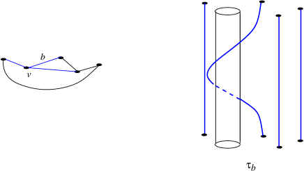
Figure 4.1. Geometric interpretation of $\tau_{b}$.

To prove the relation $\tau_{b}\sigma_{c}\sigma_{a}\tau_{b}\sigma_{c}=\sigma_{a}\tau_{b}\sigma_{c}\sigma_{a}\tau_{b}$ we add two edges $d$ and $e$, with their corresponding braids $\tau_{d}$ and $\tau_{e}$ as in Figure 4.2. The braid $\tau_{d}$ is equivalent to the braid $\sigma_{c}^{-1}\tau_{b}\sigma_{c}$ and the braid $\tau_{e}$ is equivalent to the braid $\sigma_{a}\tau_{b}\sigma_{a}^{-1}$. Then the braids $\sigma_{c}^{-1}\tau_{b}\sigma_{c}$ and $\sigma_{a}$ commute, as well as $\sigma_{a}\tau_{b}\sigma_{a}^{-1}$ and $\sigma_{c}$. So we have the following equalities, that can be easily verified on corresponding braids:

$$\tau_{b}\sigma_{c}\sigma_{a}\tau_{b}\sigma_{c}=\sigma_{c}\sigma_{c}^{-1}\tau_{b}\sigma_{c}\sigma_{a}\tau_{b}\sigma_{c}=\sigma_{c}\sigma_{a}\sigma_{c}^{-1}\tau_{b}\sigma_{c}\tau_{b}\sigma_{c}=$$

$$\sigma_{c}\sigma_{a}\sigma_{c}^{-1}\sigma_{c}\tau_{b}\sigma_{c}\tau_{b}=\sigma_{c}{\sigma_{a}\tau_{b}\sigma_{a}^{-1}}\sigma_{a}\sigma_{c}\tau_{b}=\sigma_{a}\tau_{b}\sigma_{a}^{-1}\sigma_{c}\sigma_{a}\sigma_{c}\tau_{b}=\sigma_{a}\tau_{b}\sigma_{c}\sigma_{a}\tau_{b}\,.$$

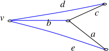
Figure 4.2. Nodal relation $\tau_{b}\sigma_{c}\sigma_{a}\tau_{b}\sigma_{c}=\sigma_{a}\tau_{b}\sigma_{c}\sigma_{a}\tau_{b}$ holds in $B_{\Gamma}(Ann)$.

Corollary 4.1.

The automorphism group of $Br_{n}(Ann)$ contains a group isomorphic to the dihedral group $D_{n-1}$.

One can associate to the graph given in Figure 4.3 a presentation for $Br_{n}(Ann)$.

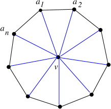
Figure 4.3. A graph associated to $Br_{n}(Ann)$.

It is possible generalize such approach to braid groups on a planar surface, i.e. a surface of genus $0$ with $l>1$ boundary components. In this case one considers a normal planar graph with $k\,(=l-1)$ distinguished vertices $v_{1},\dots,v_{k}$ such that there are no edges connecting distinguished vertices and such that the graph $\Gamma$ minus the vertices $v_{1},\dots,v_{k}$ and all the edges adjacent to $v_{1},\dots,v_{k}$ is also connected. We label by $\{\tau_{1,j},\dots,\tau_{m,j}\}$ the edges adjacent to $v_{j}$ and by $\{\sigma_{1},\dots,\sigma_{p}\}$ the edges disjoint from the set $\{v_{1},\dots,v_{k}\}$. We say that $\Gamma$ is a $k$-punctured graph. As in Theorem 4.1 one can associate to any $k$-punctured graph $\Gamma$ on $n$ vertices a set of generators for the braid group on $n$ strands on surface of genus $0$ with $k+1$ boundary components, with the above geometrical interpretation of generators.

4.2. Graph-presentations for the surface braid groups

These presentations were considered in [8]. Let $\Gamma$ be a normal graph on an orientable surface $\Sigma$ and $S(\Gamma)$ denotes the set of vertices of $\Gamma$. In the same way as earlier we associate to the edges of $\Gamma$ the corresponding geometric braids on $\Sigma$ (Figure 1.1) and we define $Br_{\Gamma}(\Sigma)$ as the subgroup of $Br_{|S(\Gamma)|}(\Sigma)$ generated by these braids.

Proposition 4.1.

Let $\Sigma$ be an oriented surface such that $\pi_{1}(\Sigma)\not=1$ and let $\Gamma$ be a normal graph on $\Sigma$. Then $Br_{\Gamma}(\Sigma)$ is a proper subgroup of $Br_{|S(\Gamma)|}(\Sigma)$.

4.3. Sphere braid groups presentations via graphs

Now let the surface $\Sigma$ be a sphere $S^{2}$ and $\Gamma$ denotes a normal finite graph on this sphere. We define a pseudocycle as in Introduction: we consider the set $S^{2}\setminus\Gamma$ as the disjoint union of a finite number of open disks $D_{1},\dots,D_{m}$, $m>1$ and define the pseudocycle associated to $D_{j}$ exactly in the same way.

Let $\Delta$ be a maximal tree of a normal graph $\Gamma$ on $q+1$ vertices. Then $\Delta$ has $q$ edges. Let $v_{1},v_{2}$ be two vertices adjacent to the same edge $\sigma$ of $\Delta$. Write $\sigma(f_{1})$ for $\sigma$. We define the circuit $\sigma(f_{1})\dots\sigma(f_{2q})$ as follows:

-if the vertex $v_{j+1}$ is not uni-valent, then $\sigma(f_{j+1})$ is the first edge on the left of $\sigma(f_{j})$ (we consider $\sigma(f_{j})$ going from $v_{j}$ to $v_{j+1}$) and the vertex $v_{j+2}$ is the other vertex adjacent to $\sigma(f_{j+1})$;

-if the vertex $v_{j+1}$ is uni-valent, then $\sigma(f_{j+1})=\sigma(f_{j})$ and $v_{j+2}=v_{j}$.

This way we come back to $v_{1}$ after passing twice through each edge of $\Delta$. Write $\delta_{v_{1},v_{2}}(\Delta)$ for the word in $X_{\Gamma}$ corresponding to the circuit $\sigma(f_{1})\dots\sigma(f_{2q})$ (Figure 4.4).

Figure 4.4. $\delta_{x,y}(\Delta)=\sigma\alpha^{2}\beta^{2}\sigma\gamma\delta^{2}\epsilon^{2}\gamma\zeta^{2}$ and $\delta_{y,x}(\Delta)=\sigma\gamma\delta^{2}\epsilon^{2}\gamma\zeta^{2}\sigma\alpha^{2}\beta^{2}$.

Theorem 4.2.

Let $\Gamma$ be a normal graph with $n$ vertices. The braid group $Br_{n}(S^{2})$ admits a presentation $\langle X_{\Gamma}\,|\,R_{\Gamma}\rangle$, where $X_{\Gamma}=\{\sigma\;|\;\sigma\;\mbox{is an edge of }\;\Gamma\}$ and $R_{\Gamma}$ is the set of following relations:

Disjointedness relations (DR); Nodal relations (NR) (Figure 1.2); Pseudocycle relations (PR) (Figure 1.3), exactly as in Theorem 1.1 and the new

Tree relations (TR): $\delta_{x,\,y}(\Delta)=1$, for every maximal tree $\Delta$ of $\Gamma$ and every ordered pair of vertices $x,y$ such that they are adjacent to the same edge $\sigma$ of $\Delta$.

Remark 4.3.

The statement of Theorem 4.2 is highly redundant. For instance one can show that a relation (TR) on a given maximal tree of $\Gamma$, together with the relations (DR), (AR), (NR) and (PR), generate the (TR) relation for any other maximal tree of $\Gamma$. Anyway, these presentations are symmetric and one can read off the relations from the geometry of $\Gamma$.

Remark 4.4.

Let $\gamma\subseteq\Gamma$ be a star (a graph which consists of several edges joined in one point). For any clockwise ordered subset $\{\sigma_{i_{1}},\dots,$ $\sigma_{i_{j}}\,|\,j\geq 2\,\}$ of edges of $\gamma$ the following relation holds in the group $\langle X_{\Gamma}\,|\,R_{\Gamma}\rangle$:

$$\sigma_{i_{1}}\dots\sigma_{i_{j}}\sigma_{i_{1}}=\sigma_{i_{j}}\sigma_{i_{1}}\dots\sigma_{i_{j}}\,.$$

4.3.1. Geometric interpretation of relations

It is geometrically evident that the relations (AR) and (DR) hold in $Br_{\Gamma}(S^{2})$. Let $\Gamma$ contain a triangle $\sigma_{1},\sigma_{2},\tau$ as in Figure 4.5.

Figure 4.5. Adding or removing a triangle.

Corresponding braids satisfy the relation $\tau=\sigma_{1}\sigma_{2}\sigma_{1}^{-1}$ and thus $\tau\sigma_{1}=\sigma_{1}\sigma_{2}$ in $Br_{\Gamma}(S^{2})$. The relation $\sigma_{1}\sigma_{2}=\sigma_{2}\tau$ follows from the braid relation $\sigma_{1}\sigma_{2}\sigma_{1}^{-1}=\sigma_{2}^{-1}\sigma_{1}\sigma_{2}$. Let $\sigma_{1},\sigma_{2},\sigma_{3}$ be arranged as in Figure 4.6. We add three edges $\tau_{1},\tau_{2},\tau_{3}$. The nodal relation follows from the pseudocycle relations on triangles $\tau_{1}\sigma_{2}\sigma_{3}$, $\tau_{2}\sigma_{1}\sigma_{3}$ and $\tau_{3}\sigma_{1}\sigma_{2}$. In fact, $\sigma_{1}\sigma_{2}\sigma_{3}\sigma_{1}=\sigma_{2}\tau_{3}\sigma_{3}\sigma_{1}=\sigma_{2}\sigma_{3}\tau_{3}\sigma_{1}=\sigma_{2}\sigma_{3}\sigma_{1}\sigma_{2}$. All other pseudocycle relations follow from induction on the length of the cycle.

Figure 4.6. Nodal relation holds in $B_{\Gamma}(S^{2})$.

Let $\Delta$ be a maximal tree of $\Gamma$. Let $\sigma$ be an edge of $\Delta$ and let $x,y$ be the two adjacent vertices. The element $\delta_{x,y}(\Delta)$ corresponds to a (pure) braid such that the braid obtained by removing the string starting from the vertex $x$ is isotopic to the trivial braid. This string goes around (with clockwise orientation) all other vertices (Figure 4.7 on the left). The braid $\delta_{x,y}(\Delta)$ is isotopic to the trivial braid in $Br_{\Gamma}(S^{2})$ and so $\delta_{x,y}(\Delta)=1$ (Figure 4.7). Therefore the natural map $\phi_{\Gamma}:\langle X_{\Gamma}\,|\,R_{\Gamma}\rangle\to Br_{\Gamma}(S^{2})$ is a homomorphism.

Figure 4.7. The braid $\delta_{x,\sigma}(\Delta)$ associated to the tree $\Delta=\Gamma\setminus\tau$.

4.4. Singular braids and graphs

As in the case of classical braids, one can extend the group $Br_{n}(\Sigma)$ to the monoid $SB_{n}(\Sigma)$ of singular braids on $n$ strands on the surface $\Sigma$. Presentations for this monoid are given in [7] and [42].

In this section we provide presentations by graphs for the monoid $SB_{n}$ and for the monoid $SB_{n}(Ann)$ of singular braids on $n$ strands of the annulus.

Let $\Gamma$ be a normal planar graph. We associate to any edge $a$ three singular braids: $\sigma_{a}$ will denote the positive half-twist associated to $a$ (as in Figure 1.1), $\sigma_{a}^{-1}$ will denote the corresponding negative half-twist and $x_{a}$ the corresponding singular crossing.

Theorem 4.3.

Let $\Gamma$ be a normal planar graph with $n$ vertices. The singular braid monoid $SB_{n}$ has the presentation $\langle X_{\Gamma},R_{\Gamma}\rangle$ where $X_{\Gamma}=$ $\{\sigma_{a},\sigma_{a}^{-1},$ $x_{a}|\ a\ \text{is an edge}$ $\text{of}\,\ \Gamma\}$ and $R_{\Gamma}$ is formed by the following six types of relations:

• disjointedness: if the edges $a$ and $b$ are disjoint, then

  $$\sigma_{a}\sigma_{b}=\sigma_{b}\sigma_{a},\;x_{a}x_{b}=x_{b}x_{a},\;\sigma_{a}x_{b}=x_{b}\sigma_{a},$$

• commutativity:

  $$\sigma_{a}x_{a}=x_{a}\sigma_{a},$$

• invertibility:

  $$\sigma_{a}\sigma_{a}^{-1}=\sigma_{a}^{-1}\sigma_{a}=1,$$

• adjacency: if the edges $a$ and $b$ have a common vertex, then

  $$\sigma_{a}\sigma_{b}\sigma_{a}=\sigma_{b}\sigma_{a}\sigma_{b},$$

  $$x_{a}\sigma_{b}\sigma_{a}=\sigma_{b}\sigma_{a}x_{b},$$

• nodal: if the edges $a$, $b$ and $c$ have a common vertex and are placed clockwise, then

  $$\sigma_{a}\sigma_{b}\sigma_{c}\sigma_{a}=\sigma_{b}\sigma_{c}\sigma_{a}\sigma_{b}=\sigma_{c}\sigma_{a}\sigma_{b}\sigma_{c},$$

  $$x_{a}\sigma_{b}\sigma_{c}\sigma_{a}=\sigma_{a}\sigma_{b}\sigma_{c}x_{a},$$

  $$\sigma_{a}\sigma_{b}x_{c}\sigma_{a}=\sigma_{b}x_{c}\sigma_{a}\sigma_{b},$$

  $$x_{a}\sigma_{b}x_{c}\sigma_{a}=\sigma_{b}x_{c}\sigma_{a}x_{b},$$

• pseudocycle: if the edges $a_{1}$, $\dots$, $a_{n}$ form an irreducible pseudocycle and if $a_{1}$ is not the starting edge nor $a_{n}$ is the end edge of a reverse, then

  $$\sigma_{a_{1}}\dots\sigma_{a_{n-1}}=\sigma_{a_{2}}\dots\sigma_{a_{n}},$$

  $$x_{a_{1}}\sigma_{a_{2}}\dots\sigma_{a_{n-1}}=\sigma_{a_{2}}\dots\sigma_{a_{n-1}}x_{a_{n}}.$$

The last aim of this section is to give graph presentations for the singular braid monoid on $n$ strands of the annulus.

Theorem 4.4.

The singular braid monoid on $n$ strands of the annulus $SB_{n}(Ann)$ admits the following presentation:

-Generators: $\sigma_{i},\sigma_{i}^{-1},x_{i}$, $(i=1,\dots,n-1),\tau,\tau^{-1}$.

-Relations:

$$(R1) \;\sigma_{i}\sigma_{j}=\sigma_{j}\sigma_{i},\;\mbox{if}\quad|i-j|>1\,;$$

$$(R2) \;x_{i}x_{j}=x_{j}x_{i},\;\mbox{if}\quad|i-j|>1\,;$$

$$(R3) \;x_{i}\sigma_{j}=\sigma_{j}x_{i},\;\mbox{if}\quad|i-j|\not=1\,;$$

$$(R4) \;\sigma_{i}\sigma_{i+1}\sigma_{i}=\sigma_{i+1}\sigma_{i}\sigma_{i+1}\,;$$

$$(R5) \;\sigma_{i}\sigma_{i+1}x_{i}=x_{i+1}\sigma_{i}\sigma_{i+1}\,;$$

$$(R6) \;\sigma_{i+1}\sigma_{i}x_{i+1}=x_{i}\sigma_{i+1}\sigma_{i}\,;$$

$$(R7) \;\tau\sigma_{1}\tau\sigma_{1}=\sigma_{1}\tau\sigma_{1}\tau\,;$$

$$(R8) \;\tau\sigma_{1}\tau x_{1}=x_{1}\tau\sigma_{1}\tau,$$

$$(R9) \;\tau\sigma_{i}=\sigma_{i}\tau,\;\mbox{if}\quad i\geq 2\,;$$

$$(R10) \;\tau x_{i}=x_{i}\tau,\;\mbox{if}\quad i\geq 2\,;$$

$$(R11) \;\sigma_{i}\sigma_{i}^{-1}=\sigma_{i}^{-1}\sigma_{i}=\tau\tau^{-1}=\tau^{-1}\tau=1.$$

The geometric interpretation of $\sigma_{i}$ and $\tau$ is given in Figure 2.1.

We get the Reidemeister moves for singular knot theory in a solid torus if we add the move depicted on Figure 4.8 to the regular (without singularities) Reidemeister moves of knot theory in a solid torus. This Reidemeister move means how a singular point goes around the axis of the torus (fixed string). The proof that the list R1-R11 is a complete set of relations is standard: every isotopy can be decomposed in a sequence of elementary isotopies which correspond to relations R1-R11 (see also [42]).

Figure 4.8. The words $\tau\sigma_{1}\tau x_{1}$ and $x_{1}\tau\sigma_{1}\tau$ represent the same element in $SB_{n}(Ann)$.

Remark 4.5.

The singular braid monoid on $n$ strands of the annulus differs from the singular Artin monoid of type $B$ as defined by R. Corran [22], where the numbers of singular and regular generators are the same. The singular generator associated to $\tau$ can not be interpreted geometrically as above.

As in Subsection 4.1 we consider 1-punctured graphs. To any edge $a$ disjoint from the distinguished vertex $v$ of $\Gamma$ we associate three singular braids: $\sigma_{a}$ will denote the positive half-twist associated to $a$, $\sigma_{a}^{-1}$ will denote the corresponding negative half-twist and $\tau_{a}$ denotes the corresponding singular crossing.

The graph presentations for the singular braid monoid in the solid torus arise from Theorems 4.3 and 4.4.

Theorem 4.5.

Let $\Gamma$ be a one-punctured graph on $n$ vertices. The monoid $SB_{n}(Ann)$ admits the presentation $\langle X_{\Gamma},R_{\Gamma}\rangle$, where

-$X_{\Gamma}=\{\sigma_{a},\sigma_{a}^{-1},x_{a},\tau_{b},\tau_{b}^{-1}\}$, for any edge $a$ of $\,\Gamma$ not incident with the distinguished vertex $v$, and for any edge $b$ of   $\Gamma$ adjacent to the distinguished vertex $v$;

- $R_{\Gamma}$ is formed by the relations given in Theorems 4.1 and 4.3 and the following new nodal and invertibility relations:

$$\sigma_{a}\tau_{b}\sigma_{c}x_{a}=x_{c}\sigma_{a}\tau_{b}\sigma_{c},$$

$$\tau_{b}\sigma_{c}\sigma_{a}\tau_{b}x_{c}=x_{a}\tau_{b}\sigma_{c}\sigma_{a}\tau_{b},$$

$$\tau_{b}\tau_{b}^{-1}=\tau_{b}^{-1}\tau_{b}=1.$$

5. Birman – Ko – Lee presentation for the singular braid monoid

The analogue of the presentation of Birman, Ko and Lee for the singular braid monoid was given in [85]. For $1\leq s<t\leq n$ and $1\leq p<q\leq n$ we consider the elements of $SB_{n}$ which are defined by

$$\begin{cases}a_{ts}&=(\sigma_{t-1}\sigma_{t-2}\cdots\sigma_{s+1})\sigma_{s}(\sigma^{-1}_{s+1}\cdots\sigma^{-1}_{t-2}\sigma^{-1}_{t-1})\ \ {\rm for}\ \ 1\leq s<t\leq n,\\ a_{ts}^{-1}&=(\sigma_{t-1}\sigma_{t-2}\cdots\sigma_{s+1})\sigma_{s}^{-1}(\sigma^{-1}_{s+1}\cdots\sigma^{-1}_{t-2}\sigma^{-1}_{t-1})\ \ {\rm for}\ \ 1\leq s<t\leq n,\\ b_{qp}&=(\sigma_{q-1}\sigma_{q-2}\cdots\sigma_{p+1})x_{p}(\sigma^{-1}_{p+1}\cdots\sigma^{-1}_{q-2}\sigma^{-1}_{q-1})\ \ {\rm for}\ \ 1\leq p<q\leq n.\end{cases}$$

Geometrically the generators $a_{s,t}$ and $b_{s,t}$ are depicted in Figure 5.1.

Figure 5.1.

Theorem 5.1.

The singular braid monoid $SB_{n}$ has a presentation with generators $a_{ts}$, $a_{ts}^{-1}$ for $1\leq s<t\leq n$ and $b_{qp}$ for $1\leq p<q\leq n$ and relations

(5.1) $$\begin{cases}a_{ts}a_{rq}&=a_{rq}a_{ts}\ \ {\rm for}\ \ (t-r)(t-q)(s-r)(s-q)>0,\\ a_{ts}a_{sr}&=a_{tr}a_{ts}=a_{sr}a_{tr}\ \ {\rm for}\ \ 1\leq r<s<t\leq n,\\ a_{ts}a_{ts}^{-1}&=a_{ts}^{-1}a_{ts}=1\ \ {\rm for}\ \ 1\leq s<t\leq n,\\ a_{ts}b_{rq}&=b_{rq}a_{ts}\ \ {\rm for}\ \ (t-r)(t-q)(s-r)(s-q)>0,\\ a_{ts}b_{ts}&=b_{ts}a_{ts}\ \ {\rm for}\ \ 1\leq s<t\leq n,\\ a_{ts}b_{sr}&=b_{tr}a_{ts}\ \ {\rm for}\ \ 1\leq r<s<t\leq n,\\ a_{sr}b_{tr}&=b_{ts}a_{sr}\ \ {\rm for}\ \ 1\leq r<s<t\leq n,\\ a_{tr}b_{ts}&=b_{sr}a_{tr}\ \ {\rm for}\ \ 1\leq r<s<t\leq n,\\ b_{ts}b_{rq}&=b_{rq}b_{ts}\ \ {\rm for}\ \ (t-r)(t-q)(s-r)(s-q)>0.\end{cases}$$

Now we consider the positive singular braid monoid $SBKL_{n}^{+}$ with respect to generators $a_{ts}$ and $b_{t,s}$ for $1\leq s<t\leq n$. Its relations are (5.1) except the one concerning the invertibility of $a_{ts}$. Two positive words $A$ and $B$ in the alphabet $a_{ts}$ and $b_{t,s}$ will be said to be positively equivalent if they are equal as elements of this monoid. In this case we shall write $A\doteq B$.

The fundamental word $\delta$ of Birman, Ko and Lee is given by the formula

$$\delta\equiv a_{n(n-1)}a_{(n-1)(n-2)}\dots a_{21}\equiv\sigma_{n-1}\sigma_{n-2}\dots\sigma_{2}\sigma_{1}.$$

Its divisibility by any generator $a_{ts}$, proved in [14], is convenient for us to be expressed in the following form.

Proposition 5.1.

The fundamental word $\delta$ is positively equivalent to a word that begins or ends with any given generator $a_{ts}$. The explicit expression for left divisibility is

$$\delta\doteq a_{ts}a_{n(n-1)}a_{(n-1)(n-2)}\dots a_{(t+1)s}a_{t(t-1)}\dots a_{(s+2)(s+1)}a_{s(s-1)}\dots a_{21}.$$

Proposition 5.2.

For the fundamental word $\delta$ there are the following formulae of commutation

$$\begin{cases}a_{ts}\delta&\doteq\delta a_{(t+1)(s+1)}\ \ \text{for}\ \ 1\leq s<t<n,\\ a_{ns}\delta&\doteq\delta a_{(s+1)1},\\ b_{ts}\delta&\doteq\delta b_{(t+1)(s+1)}\ \ \text{for}\ \ 1\leq s<t<n,\\ b_{ns}\delta&\doteq\delta b_{(s+1)1}.\end{cases}$$

Geometrically this commutation is shown on Figure 5.2 and on Figure 5.3.

Figure 5.2.

Figure 5.3.

The analogues of the other results proved by Birman, Ko and Lee remain valid for the singular braid monoid. They are proved in the work of V. V. Chaynikov [20].

6. The work of V. V. Chaynikov

6.1. Cancellation property

Let $W_{1},W_{2}\in$$SBKL_{n}^{+}$. By a common multiple of $W_{1},W_{2}$ (if it exists) we mean a positive word $V\doteq W_{1}V_{1}\doteq W_{2}V_{2}$.

Let

$$\delta_{s_{k}...s_{1}}\equiv a_{s_{k}s_{(k-1)}}a_{s_{(k-1)}s_{(k-2)}}\dots a_{s_{21}},$$

where $n\geq s_{k}>s_{k-1}>\dots>s_{1}\geq 1$. The word $\delta_{s_{k}...s_{1}}$ is the least common multiple (l.c.m.) of the generators $a_{ij}$, where $i,j\in\{s_{k},s_{(k-1)},\dots s_{1}\}$, see [14], $\delta\equiv\delta_{n(n-1)\dots 1}$.

We denote the least common multiple of $X,Y$ by $X\vee Y$. Define $(X\vee Y)_{X}^{*}$ and $(X\vee Y)_{Y}^{*}$ by equations:

$$X\vee Y\doteq X(X\vee Y)_{X}^{*}\doteq Y(X\vee Y)_{Y}^{*}.$$

Similarly, we denote the greatest common divisor (g.c.d.) of $X,Y$ by $X\wedge Y$. The semigroup $BKL_{n}^{+}$ is a lattice relative to $\vee,\wedge$ [14].

Remark 6.1.

We give the table of l.c.m. for some pairs of generators below. There does not exist $X\vee Y$ for the rest pairs of $SBKL_{n}^{+}$ generators.

$X$	$Y$	$X\vee Y$
$\hat{a}_{ts}$	$\hat{a}_{rq}$	$\hat{a}_{ts}(\hat{a}_{rq})\doteq\hat{a}_{rq}(\hat{a}_{ts})$	$(t-r)(t-q)(s-r)(s-q)>0$
		$a_{ts}(a_{sr})\doteq a_{tr}(a_{ts})\doteq a_{sr}(a_{tr})$	$t>s>r$
$a_{ts}$	$a_{rq}$	$a_{ts}a_{tr}a_{sq}\doteq a_{rq}a_{tq}(a_{rs})\doteq\delta_{trsq}$	$t>r>s>q$
$a_{ts}$	$b_{ts}$	$a_{ts}(b_{ts})\doteq b_{ts}(a_{ts})$	$t>s>r$
$a_{sr}$	$b_{tr}$	$a_{ts}(b_{sr})\doteq b_{tr}(a_{ts})$	$t>s>r$
$a_{sr}$	$b_{ts}$	$a_{sr}(b_{tr})\doteq b_{ts}(a_{sr})$	$t>s>r$
$a_{ts}$	$b_{sr}$	$a_{ts}(a_{sr}b_{ts})\doteq b_{sr}(\delta_{tsr})$	$t>s>r$
$a_{sr}$	$b_{tr}$	$a_{sr}(a_{tr}b_{sr})\doteq b_{tr}(\delta_{tsr})$	$t>s>r$
$a_{tr}$	$b_{ts}$	$a_{tr}(a_{ts}b_{tr})\doteq b_{ts}(\delta_{tsr})$	$t>s>r$
$a_{ts}$	$b_{rq}$	$a_{ts}(\delta_{trq}b_{ts})\doteq b_{ts}(\delta_{trsq})$	$t>r>s>q$
$a_{rq}$	$b_{ts}$	$a_{rq}(a_{tq}a_{rs}b_{rq})\doteq b_{ts}(\delta_{trsq})$	$t>r>s>q$

Here the symbol $\hat{a}_{ij}\in\{a_{ij},\ b_{ij}\}$, mean the same symbol in both parts of one equality.

We call the pairs of generator from the table above admissible and all other pairs inadmissible. Observe that pairs $\{a_{ij}$, $a_{pm}\}$, $\{a_{ij},b_{pm}\}$ are admissible and $\{b_{ij},b_{pm}\}$ is admissible if and only if $b_{ij}b_{pm}=b_{pm}b_{ij}$ is the defining relation of $SB_{n}$.

Theorem 6.1 (Left cancellation).

i)Let $\{x,y\}$ be an admissible pair and $xX\doteq yY$. Then there exists a positive word $Z$ such that $xX\doteq yY\doteq(x\vee y)Z$, where $X\doteq(x\vee y)_{x}^{*}Z$ and $Y\doteq(x\vee y)_{y}^{*}Z$.

ii) If the pair $\{x,y\}$ is inadmissible then the equality $xX\doteq yY$ is impossible (so there does not exist a common multiple for $\{x,y\}$).

Similarly we can obtain the Right cancellation property.

Corollary 6.1.

If $A\doteq P$, $B\doteq Q$, $AXB\doteq PYQ$, then the equality $X\doteq Y$ holds in $SBKL_{n}^{+}$.

Corollary 6.2.

Suppose that $\delta$ is the l.c.m. of the set of generators $\{a_{i_{1}j_{1}},\dots,a_{i_{p}j_{p}}\}$ and $W$ is a positive word such that either

$$W\doteq a_{i_{1}j_{1}}A_{1}\doteq a_{i_{2}j_{2}}A_{2}\doteq\dots\doteq a_{i_{p}j_{p}}A_{p},$$

or

$$W\doteq B_{1}a_{i_{1}j_{1}}\doteq B_{2}a_{i_{2}j_{2}}\doteq\dots\doteq B_{p}a_{i_{p}j_{p}},$$

then $W\doteq\delta Z$ for some positive word $Z$.

Corollary 6.3 (Embedding theorem).

The canonical homomorphism

$$SBKL_{n}^{+}\to SB_{n}$$

is injective.

6.2. Word and conjugacy problems in $SB_{n}$

The word problem in $SB_{n}$ (in classical generators) was solved by R. Corran [22], see also [85]. Let us fix an arbitrary linear order on the set of generators of $SBKL_{n}^{+}$  and extend it to the deg–lex order on words of the generators of $SBKL_{n}^{+}$. With this order, we first order wwords by total degree (the length of the word on given generators) and we break ties by the lex order. By the base of the positive word $W$ we mean the least (relative to the deg–lex order on the words on the generators of $SBKL_{n}^{+}$) word which represents the same element as $W$ in $SBKL_{n}^{+}$. Observe that this word is unique. If the positive word $A$ is not divisible by $\delta$ we denote its base by $\overline{A}$.

Theorem 6.2.

Every word $W$ in $SB_{n}$ has a unique representation of shape $\delta^{m}\overline{A}$, where $m$ is an integer and $A$ is not divisible by $\delta$ .

This gives a normal form for $SB_{n}$ in Birman–Ko–Lee  generators. The process of computation of this normal form is the same as given by Garside [37]. First, suppose that $P$ is any positive word in the generators $SBKL_{n}^{+}$. Among all positive words positively equivalent to $P$ choose a word in the form $\delta^{t}A$ with $t$ maximal. Then $A$ is prime to $\delta$ and we have

$$P\doteq\delta^{t}\overline{A}.$$

Now, let $W$ be an arbitrary word in $SB_{n}$. Then we may put

$$W\equiv W_{1}(c_{1})^{-1}W_{2}(c_{2})^{-1}\dots(c_{k})^{-1}W_{k+1},$$

where each $W_{j}$ is a positive word of length $\geq 0$, and $c_{l}$ are generators $a_{t,s}$, the only possible invertible generators. For each $c_{l}$ there exists a positive word $D_{l}$ such that $c_{l}D_{l}\doteq\delta$, so that $(c_{l})^{-1}=D_{l}\delta^{-1}$, and hence

$$W=W_{1}D_{1}\delta^{-1}W_{2}D_{2}\delta^{-1}\dots W_{k}D_{k}\delta^{-1}W_{k+1}.$$

Moving the factors $\delta^{-1}$ to the left, we obtain $W=\delta^{k}P$, where $P$ is positive, so we can express it in the form $\delta^{t}\overline{A}$ and finally we obtain the normal form

$$W=\delta^{m}\overline{A}.$$

Let us consider the conjugacy problem. We say that two elements $u,v\in SB_{n}$ are conjugated if there exists $g\in B_{n}$ such that $g^{-1}ug=v$. We denote this by $u\sim v$.

Let $u$ be a positive word. Define the set of all positive elements conjugated with $u$ as follows $C^{+}(u)=\{v|v\sim u,v\in SBKL_{n}^{+}\}$.

The following properties are obvious and very close to the ones proved in [29], [14]:

i) The set of all positive words of limited length is finite.

ii)The set $C^{+}(u)$ is finite.

iii)The element $\delta^{n}$ generates the center of $SB_{n}$.

Now fix two words $u,v\in SB_{n}$. We can assume that they are positive (otherwise we multiply them by the element $\delta^{nk}$, where $k$ is big enough to cancel all negative letters).

Theorem 6.3.

The elements $u,v$ are conjugated if and only if the sets $C^{+}(u)$ and $C^{+}(v)$ contain the same elements.

There exists the following algorithm for constructing $C^{+}(u)$. Define $C_{0}^{+}(u):=\{u\}$. If the set $C_{i}^{+}(u)$ is already constructed define

$$C_{i+1}^{+}(u):=\{v^{g}\ |\ g\text{ divides}\ \delta;\ v\in C_{i}^{+}\}\cap SBKL_{n}^{+}.$$

The set $C_{k}^{+}(u)$ stabilizes on the finite step, so we put

$$C^{+}(u):=\bigcup_{k\geq 0}C_{k}^{+}(u).$$

7. Inverse monoids

The notion of inverse semigroup was introduced by V. V. Wagner in 1952 [87]. By definition it means that for any element $a$ of a semigroup (monoid) $M$ there exists a unique element $b$ (which is called inverse) with the following two conditions:

(7.1) $$a=aba$$

(7.2) $$b=bab.$$

Roots of this notion can be seen in the von Neumann regular rings [61] where only one condition (7.1) holds for non-necessary unique $b$, or in the Moore-Penrose pseudoinverse for matrices [60], [64] where both conditions (7.1) and (7.2) hold (and certain supplementary conditions also). See the books [65] and [53] as general references for inverse semigroups.

The typical example of an inverse monoid is a monoid of partial (defined on a subset) injections of a set. For a finite set this gives us the notion of a symmetric inverse monoid $I_{n}$ which generalizes and includes the classical symmetric group $\Sigma_{n}$. A presentation of symmetric inverse monoid was obtained by L. M. Popova [67], see also formulae (7.3 -7.4) below.

Recently the inverse braid monoid $IB_{n}$ was constructed by D. Easdown and T. G. Lavers [28]. It arises from a very natural operation on braids: deleting one or several strands. By the application of this procedure to braids in $Br_{n}$ we get partial braids [28]. The multiplication of partial braids is shown at Figure 7.1 At the last stage it is necessary to remove any arc that does not join the upper or lower planes. The set of all partial braids with this operation forms an inverse braid monoid $IB_{n}$.

One of the motivations for studying $IB_{n}$ is that it is a natural setting for the Brunnian (or Makanin) braids, which were also called smooth braids by G. S. Makanin who first mentioned them in [49], (page 78, question 6.23), and D. L. Johnson [45]. By the usual definition a braid is Brunnian if it becomes trivial after deleting any strand, see formulae (8.9 - 8.13). According to the work of Fred Cohen, Jon Berrick, Wu Jie, Yang Loi Wong [10] Brunnian braids are connected with homotopy groups of spheres.

Figure 7.1.

The following presentation for the inverse braid monoid was obtained in [28]. It has the generators $\sigma_{i},\sigma_{i}^{-1}$, $i=1,\dots,n-1,$ $\epsilon$, which satisfy the braid relations (1.1 and the following relations:

(7.3) $$\begin{cases}&\sigma_{i}\sigma_{i}^{-1}=\sigma_{i}^{-1}\sigma_{i}=1,\ \text{for \ all}\ i,\\ &\epsilon\sigma_{i}=\,\sigma_{i}\epsilon\ \ \text{for }i\geq 2,\\ &\epsilon\sigma_{1}\epsilon=\sigma_{1}\epsilon\sigma_{1}\epsilon=\epsilon\sigma_{1}\epsilon\sigma_{1},\\ &\epsilon=\epsilon^{2}=\epsilon\sigma_{1}^{2}=\sigma_{1}^{2}\epsilon.\end{cases}$$

Geometrically the generator $\epsilon$ means that the first strand in the trivial braid is absent.

If we replace the first relation in (7.3) by the following set of relations

(7.4) $$\sigma_{i}^{2}=1,\ \text{for \ all}\ i,\\$$

and delete the superfluous relations

$$\epsilon=\epsilon\sigma_{1}^{2}=\sigma_{1}^{2}\epsilon,$$

we get a presentation of the symmetric inverse monoid $I_{n}$ [67]. We also can simply add the relations (7.4) if we do not worry about redundant relations. We get a canonical map [28]

(7.5) $$\tau_{n}:IB_{n}\to I_{n}$$

which is a natural extension of the corresponding map for the braid and symmetric groups.

More balanced relations for the inverse braid monoid were obtained in [40]. Let $\epsilon_{i}$ denote the braid which is obtained from the trivial by deleting of the $i$th strand, formally:

$$\begin{cases}\epsilon_{1}&=\epsilon,\\ \epsilon_{i+1}&=\sigma_{i}^{\pm 1}\epsilon_{i}\sigma_{i}^{\pm 1}.\end{cases}$$

So, the generators are: $\sigma_{i},\sigma_{i}^{-1}$, $i=1,\dots,n-1,$ $\epsilon_{i}$, $i=1,\dots,n$, and relations are the following:

(7.6) $$\begin{cases}&\sigma_{i}\sigma_{i}^{-1}=\sigma_{i}^{-1}\sigma_{i}=1,\ \text{for all}\ i,\\ &\epsilon_{j}\sigma_{i}=\,\sigma_{i}\epsilon_{j}\ \ \text{for }\ j\not=i,i+1,\\ &\epsilon_{i}\sigma_{i}=\sigma_{i}\epsilon_{i+1},\\ &\epsilon_{i+1}\sigma_{i}=\sigma_{i}\epsilon_{i},\\ &\epsilon_{i}=\epsilon_{i}^{2},\\ &\epsilon_{i+1}\sigma_{i}^{2}=\sigma_{i}^{2}\epsilon_{i+1}=\epsilon_{i+1},\\ &\epsilon_{i}\epsilon_{i+1}\sigma_{i}=\sigma_{i}\epsilon_{i}\epsilon_{i+1}=\epsilon_{i}\epsilon_{i+1},\end{cases}$$

plus the braid relations (1.1).

7.1. Inverse reflection monoid of type $B$

It can be defined in the same way as the corresponding Coxeter group (2.1) as the monoid of partial signed permutations $I(B_{n})$:

$$I(B_{n})=\{\sigma\text{ is a partial bijection of }SN:(-x)\sigma=-(x)\sigma\text{ for}\ x\in SN\\ \text{and }x\in\operatorname{dom}\sigma\ \text{if and only if}-x\in\operatorname{dom}\sigma\},$$

where $\operatorname{dom}\sigma$ means domain of definition of the monomorphism $\sigma$. This monoid was studied in [31].

8. Properties of inverse braid monoid

In relations (7.3) we have one generator for the idempotent part and $n-1$ generators for the group part. If we minimize the number of generators of the group part and take the presentation (1.5) for the braid group we get a presentation of the inverse braid monoid with generators $\sigma_{1},\sigma$, $\epsilon$, and relations:

$$\begin{cases}&\sigma_{1}\sigma_{1}^{-1}=\sigma_{1}^{-1}\sigma_{1}=1,\\ &\sigma\sigma^{-1}=\sigma^{-1}\sigma=1,\\ &\epsilon\sigma^{i}\sigma_{1}\sigma^{-i}=\,\sigma^{i}\sigma_{1}\sigma^{-i}\epsilon\ \ \text{for }1\leq i\leq n-2,\\ &\epsilon\sigma_{1}\epsilon=\sigma_{1}\epsilon\sigma_{1}\epsilon=\epsilon\sigma_{1}\epsilon\sigma_{1},\\ &\epsilon=\epsilon^{2}=\epsilon\sigma_{1}^{2}=\sigma_{1}^{2}\epsilon,\end{cases}$$

plus (1.5).

Let $\Gamma$ be a normal planar graph (see Introduction). Let us add new generators $\epsilon_{v}$ which correspond to each vertex of the graph $\Gamma$. Geometrically it means the absence in the trivial braid of one strand corresponding to the vertex $v$. We orient the graph $\Gamma$ arbitrarily and so we get a starting $v_{0}=v_{0}(e)$ and a terminal $v_{1}=v_{1}(e)$ vertex for each edge $e$. Consider the following relations

(8.1) $$\begin{cases}&\sigma_{e}\sigma_{e}^{-1}=\sigma_{e}^{-1}\sigma_{e}=1,\ \text{for all edges of}\ \Gamma,\\ &\epsilon_{v}\sigma_{e}=\,\sigma_{e}\epsilon_{v},\ \ \text{if the vertex }\ v\ \text{and the edge}\ e\ \text{do not intersect},\\ &\epsilon_{v_{0}}\sigma_{e}=\sigma_{e}\epsilon_{v_{1}},\ \text{where}\ v_{0}=v_{0}(e),\ v_{1}=v_{1}(e),\\ &\epsilon_{v_{1}}\sigma_{e}=\sigma_{e}\epsilon_{v_{0}},\\ &\epsilon_{v}=\epsilon_{\nu}^{2},\\ &\epsilon_{v_{i}}\sigma_{e}^{2}=\sigma_{e}^{2}\epsilon_{v_{i}}=\epsilon_{v_{i}},\ \ i=0,1,\\ &\epsilon_{v_{0}}\epsilon_{v_{1}}\sigma_{e}=\sigma_{e}\epsilon_{v_{0}}\epsilon_{v_{1}}=\epsilon_{v_{0}}\epsilon_{v_{1}}.\end{cases}$$

Theorem 8.1.

We get a Sergiescu graph presentation of the inverse braid monoid $IB_{n}$ if we add to the graph presentation of the braid group $Br_{n}$ relations (8.1).

Let $EF_{n}$ be a monoid of partial isomorphisms of a free group $F_{n}$ defined as follows. Let $a$ be an element of the symmetric inverse monoid $I_{n}$, $a\in I_{n}$, $J_{k}=\{j_{1},\dots,j_{k}\}$ is the image of $a$, and elements $i_{1},\dots,i_{k}$ belong to domain of the definition of $a$. The monoid $EF_{n}$ consists of isomorphisms of free subgroups

$$<x_{i_{1}},\dots,x_{i_{k}}>\,\to\ <x_{j_{1}},\dots,x_{j_{k}}>$$

such that

$$f_{a}:x_{i}\mapsto w_{i}^{-1}x_{a(i)}w_{i},$$

if $i$ is among $i_{1},\dots,i_{k}$ and not defined otherwise and $w_{i}$ is a word on $x_{j_{1}},\dots,x_{j_{k}}$. The composition of $f_{a}$ and $g_{b}$, $a,b\in I_{n}$, is defined for $x_{i}$ belonging to the domain of $a\circ b$. We put $x_{j_{m}}=1$ in a word $w_{i}$ if $x_{j_{m}}$ does not belong to the domain of definition of $g$. We define a map $\phi_{n}$ from $IB_{n}$ to $EF_{n}$ expanding the canonical inclusion

$$Br_{n}\to\operatorname{Aut}F_{n}$$

by the condition that $\phi_{n}(\epsilon)$ as a partial isomorphism of $F_{n}$ is given by the formula

(8.2) $$\phi_{n}(\epsilon)(x_{i})=\begin{cases}x_{i}{\text{ if}}\ i\geq 2,\\ {\text{not defined, if }}i=1.\end{cases}$$

Using the presentation (7.3) we see that $\phi_{n}$ is correctly defined homomorphism of monoids

$$\phi_{n}:IB_{n}\to EF_{n}.$$

Theorem 8.2.

The homomorphism $\phi_{n}$ is a monomorphism.

Theorem 8.2 gives also a possibility to interpret the inverse braid monoid as a monoid of isotopy classes of maps. As usual consider a disc $D^{2}$ with $n$ fixed points. Denote the set of these points by $Q_{n}$. The fundamental group of $D^{2}$ with these points deleted is isomorphic to $F_{n}$. Consider homeomorphisms of $D^{2}$ onto a copy of the same disc with the condition that only $k$ points of $Q_{n}$, $k\leq n$ (say $i_{1},\dots,i_{k}$) are mapped bijectively onto the $k$ points (say $j_{1},\dots,j_{k}$) of the second copy of $D^{2}$. Consider the isotopy classes of such homeomorphisms and denote such set by $IM_{n}(D^{2})$. Evidently it is a monoid.

Theorem 8.3.

The monoids $IB_{n}$ and $IM_{n}(D^{2})$ are isomorphic.

These considerations can be generalized to the following definition. Consider a surface $S_{g,b,n}$ of the genus $g$, $b$ boundary components and with a chosen set $Q_{n}$ of $n$ fixed interior points. Let $f$ be a homeomorphism of $S_{g,b,n}$ which maps $k$ points, $k\leq n$, from $Q_{n}$: $\{i_{1},\dots,i_{k}\}$ to $k$ points $\{j_{1},\dots,j_{k}\}$ also from $Q_{n}$. In the same way let $h$ be a homeomorphism of $S_{g,b,n}$ which maps $l$ points, $l\leq n$, from $Q_{n}$, say $\{s_{1},\dots,s_{l}\}$ to $l$ points $\{t_{1},\dots,t_{l}\}$ again from $Q_{n}$. Consider the intersection of the sets $\{j_{1},\dots,j_{k}\}$ and $\{s_{1},\dots,s_{l}\}$, let it be the set of cardinality $m$, it may be empty. Then the composition of $f$ and $h$ maps $m$ points of $Q_{n}$ to $m$ points (may be different) of $Q_{n}$. If $m=0$ then the composition does not take into account the set $Q_{n}$. Denote the set of isotopy classes of such maps by $\mathcal{I}\mathcal{M}_{g,b,n}$. This standard composition of $f$ and $g$ as maps defines a structure of monoid on $\mathcal{I}\mathcal{M}_{g,b,n}$.

Proposition 8.1.

The monoid $\mathcal{I}\mathcal{M}_{g,b,n}$ is inverse.

We call the monoid $\mathcal{I}\mathcal{M}_{g,b,n}$ the inverse mapping class monoid. If $g=0$ and $b=1$ we get the inverse braid monoid. In the general case $\mathcal{I}\mathcal{M}_{g,b,n}$ the role of the empty braid plays the mapping class group $\mathcal{M}_{g,b}$ (without fixed points).

We remind that a monoid $M$ is factorisable if $M=EG$ where $E$ is a set of idempotents of $M$ and $G$ is a subgroup of $M$.

Proposition 8.2.

The monoid $\mathcal{I}\mathcal{M}_{g,b,n}$ can be written in the form

$$\mathcal{I}\mathcal{M}_{g,b,n}=E\mathcal{M}_{g,b,n},$$

where $E$ is a set of idempotents of $\mathcal{I}\mathcal{M}_{g,b,n}$ and $\mathcal{M}_{g,b,n}$ is the corresponding mapping class group. So this monoid is factorisable.

Let $\Delta$ be the Garside’s fundamental word in the braid group $Br_{n}$ [37]. It can be defined by the formula:

$$\Delta=\sigma_{1}\dots\sigma_{n-1}\sigma_{1}\dots\sigma_{n-2}\dots\sigma_{1}\sigma_{2}\sigma_{1}.$$

Proposition 8.3.

The generators $\epsilon_{i}$ commute with $\Delta$ in the following way:

$$\epsilon_{i}\Delta=\Delta\epsilon_{n+1-i}.$$

Proposition 8.4.

The center of $IB_{n}$ consists of the union of the center of the braid group $Br_{n}$ (generated by $\Delta^{2}$) and the empty braid $\varnothing=\epsilon_{1}\dots\epsilon_{n}$.

Let $\mathcal{E}$ be the monoid generated by one idempotent generator $\epsilon$ .

Proposition 8.5.

The abelianization of $IB_{n}$ is isomorphic to an abelian monoid ${AB}$ generated (as an abelian monoid) by elements $\epsilon$, $\alpha$ and $-\alpha$, subject to the following relations

$$\begin{cases}\alpha+(-\alpha)=0,\\ 2\epsilon=\epsilon,\\ \epsilon+\alpha=\epsilon.\end{cases}$$

So, it is isomorphic to the quotient-monoid of $\mathcal{E}\oplus\mathbb{Z}$ by the relation $\epsilon+1=\epsilon$. The canonical map of abelianization

$$a:{IB}_{n}\to{AB}$$

is given by the formula:

$$\begin{cases}a(\epsilon_{i})=\epsilon,\\ a(\sigma_{i})={\alpha}.\end{cases}$$

Let $\epsilon_{k+1,n}$ denote the partial braid with the trivial first $k$ strands and the absent rest $n-k$ strands. It can be expressed using the generator $\epsilon$ or the generators $\epsilon_{i}$ as follows

(8.3) $$\epsilon_{k+1,n}=\epsilon\sigma_{n-1}\dots\sigma_{k+1}\epsilon\sigma_{n-1}\dots\sigma_{k+2}\epsilon\dots\epsilon\sigma_{n-1}\sigma_{n-2}\epsilon\sigma_{n-1}\epsilon,$$

(8.4) $$\epsilon_{k+1,n}=\epsilon_{k+1}\epsilon_{k+2}\dots\epsilon_{n},$$

It was proved in [28] the every partial braid has a representative of the form

(8.5) $$\sigma_{i_{1}}\dots\sigma_{1}\dots\sigma_{i_{k}}\dots\sigma_{k}\epsilon_{k+1,n}x\epsilon_{k+1,n}\sigma_{k}\dots\sigma_{j_{k}}\dots\sigma_{1}\dots\sigma_{j_{1}},\\$$

(8.6) $$k\in\{0,\dots,n\},x\in Br_{k},0\leq i_{1}<\dots<i_{k}\leq n-1\ \text{and}\ 0\leq j_{1}<\dots<j_{k}\leq n-1.$$

Note that in the formula (8.5) we can delete one of the $\epsilon_{k+1,n}$, but we shall use the form (8.5) because of convenience: two symbols $\epsilon_{k+1,n}$ serve as markers to distinguish the elements of $Br_{k}$. We can put the element $x\in Br_{k}$ in the Markov normal form [58] and get the corresponding Markov normal form for the inverse braid monoid $IB_{n}$.

Among positive words on the alphabet $\{\sigma_{1}\dots\sigma_{n}\}$ let us introduce a lexicographical ordering with the condition that $\sigma_{1}<\sigma_{2}<\dots<\sigma_{n}$. For a positive word $V$ the base of $V$ is the smallest positive word which is positively equal to $V$. The base is uniquely determined. If a positive word $V$ is prime to $\Delta$, then for the base of $V$ the notation $\overline{V}$ will be used (compare with subsection 6.2).

Theorem 8.4.

Every word $W$ in $IBr_{n}$ can be uniquely written in the form

(8.7) $$\sigma_{i_{1}}\dots\sigma_{1}\dots\sigma_{i_{k}}\dots\sigma_{k}\epsilon_{k+1,n}x\epsilon_{k+1,n}\sigma_{k}\dots\sigma_{j_{k}}\dots\sigma_{1}\dots\sigma_{j_{1}},\\$$

(8.8) $$k\in\{0,\dots,n\},x\in Br_{k},0\leq i_{1}<\dots<i_{k}\leq n-1\ \text{and}\ 0\leq j_{1}<\dots<j_{k}\leq n-1.$$

where $x$ is written in the Garside normal form for $Br_{k}$

$$\Delta^{m}\overline{V},$$

where $m$ is an integer.

Theorem 8.4 is evidently true also for the presentation with $\epsilon_{i}$, $i=1,\dots n$. In this case the elements $\epsilon_{k+1,n}$ are expressed by (8.4).

We call the form of a word $W$ established in Theorem 8.4 the Garside left normal form for the inverse braid monoid $IB_{n}$ and the index $m$ we call the power of $W$. In the same way we can define the Garside right normal form for the inverse braid monoid and the corresponding variant of Theorem 8.4 is true.

Theorem 8.5.

The necessary and sufficient condition for two words in $IB_{n}$ to be equal is that their Garside normal forms are identical. The Garside normal form gives a solution to the word problem in the braid group.

Garside normal form for the braid groups was detailed in the subsequent works of S. I. Adyan [1], W. Thurston [30], E. El-Rifai and H. R. Morton [29]. Namely, there was introduced the left-greedy form (in the terminology of W. Thurston [30])

$$\Delta^{t}A_{1}\dots A_{k},$$

where $A_{i}$ are the successive possible longest fragments of the word $\Delta$ (in the terminology of S. I. Adyan [1]) or positive permutation braids (in the terminology of E. El-Rifai and H. R. Morton [29]). In the same way one defines the right-greedy form is defined. These greedy forms are defined for the inverse braid monoid in the same way.

Let us consider the elements $m\in IB_{n}$ satisfying the equation:

(8.9) $$\epsilon_{i}m=\epsilon_{i}.$$

Geometrically this means that removing the strand (if it exists) that starts at the point with the number $i$ we get a trivial braid on the remaining $n-1$ strands. It is equivalent to the condition

(8.10) $$m\epsilon_{\tau(m)(i)}=\epsilon_{\tau(m)(i)},$$

where $\tau$ is the canonical map to the symmetric monoid (7.5). With the exception of $\epsilon_{i}$ itself all such elements belong to $Br_{n}$. We call such braids as $i$ -Brunnian and denote the subgroup of $i$ -Brunnian braids by $A_{i}$. The subgroups $A_{i}$, $i=1,\dots,n$, are conjugate

(8.11) $$A_{i}=\sigma_{i-1}^{-1}\dots\sigma_{1}^{-1}A_{1}\sigma_{1}\dots\sigma_{i-1}$$

free subgroups. The group $A_{1}$ is freely generated by the set $\{x_{1},\dots,x_{n-1}\}$ [45], where

(8.12) $$x_{i}=\sigma_{i-1}^{-1}\dots\sigma_{1}^{-1}\sigma_{1}^{2}\sigma_{1}\dots\sigma_{i-1}.$$

The intersection of all subgroups of $i$ -Brunnian braids is the group of Brunnian braids

(8.13) $$Brunn_{n}=\cap_{i=1}^{n}A_{i}.$$

That is the same as $m\in Brunn_{n}$ if and only if the equation (8.9) holds for all $i$.

9. Monoids of partial generalized braids

Construction of partial braids can be applied to various generalizations of braids, namely to those where geometric or diagrammatic construction of braids takes place. Let $\Sigma_{g}$ be a surface of genus $g$ possibly with boundary components and punctures. We consider partial braids lying in a layer between two such surfaces: $\Sigma_{g}\times I$ and take a set of isotopy classes of such braids. We get a monoid of partial braid on a surface $\Sigma_{g}$, denote it by $IB_{n}(\Sigma_{g})$. An interesting case is when the surface is a sphere $S^{2}$. So our partial braids are lying in a layer between two concentric spheres.

Theorem 9.1.

We get a presentation of the monoid $IB_{n}(S^{2})$ if we add to the presentation (7.3) or to the presentation (7.6) of $IB_{n}$ the sphere relation (2.4). It is a factorisable inverse monoid.

The monoid $IB(B_{n})$ of partial braids of the type $B$ can be considered also as a submonoid of $IB_{n+1}$ consisting of partial braids with the first strand fixed. An interpretation as a monoid of isotopy classes of homeomorphisms is possible as well. Consider a disc $D^{2}$ with given $n+1$ points. Denote the set of these points by $Q_{n+1}$. Consider homeomorphisms of the disc $D^{2}$ onto a copy of the same disc with the condition that the first point is always mapped into itself and among the other $n$ points only $k$ points, $k\leq n$ (say $i_{1},\dots,i_{k}$) are mapped bijectively onto the $k$ points (say $j_{1},\dots,j_{k}$) of the set $Q_{n+1}$ (without the first point) of second copy of the disc $D^{2}$. The isotopy classes of such homeomorphisms form the monoid $IB(B_{n})$.

Theorem 9.2.

We get a presentation of the monoid $IB(B_{n})$ if we add to the presentation (7.3) or the presentation (7.6) of $IB_{n}$ one generator $\tau$, the type $B$ relation (2.2) and the following relations

(9.1) $$\begin{cases}&\tau\tau^{-1}=\tau^{-1}\tau=1,\\ &\epsilon_{1}\tau=\tau\epsilon_{1}=\epsilon_{1}.\end{cases}$$

It is a factorisable inverse monoid.

Remark 9.1.

Theorem 9.2 can be naturally generalized for partial braids in handlebodies [77].

We define an action of the monoid ${IB}(B_{n})$ on the set $SN$ (see subsection 2.1) by partial isomorphisms as follows

(9.2) $$\sigma_{i}(\delta_{j}v_{j})=\begin{cases}\delta_{i}v_{i+1},\ \text{if }j=i,\\ \delta_{i+1}v_{i},\ \text{if }j=i+1,\\ \delta_{j}v_{j},\ \text{if }j\not=i,i+1,\\ \end{cases}$$

(9.3) $$\tau(\delta_{j}v_{j})=\begin{cases}-\delta_{1}v_{1},\ \text{if }j=1,\\ \delta_{j}v_{j},\ \text{if }j\not=1,\\ \end{cases}$$

(9.4) $$\operatorname{dom}\epsilon=\{\delta_{2}v_{2},\dots,\delta_{n}v_{n}\},$$

(9.5) $$\epsilon(\delta_{j}v_{j})=\delta_{j}v_{j},\ \text{if }j=2,\dots,n,\\$$

(9.6) $$\operatorname{dom}\epsilon_{i}=\{\delta_{1}v_{1},\dots,{\widehat{\delta_{i}v_{i}}},\dots,\delta_{n}v_{n}\},$$

(9.7) $$\epsilon_{i}(\delta_{j}v_{j})=\delta_{j}v_{j},\ \text{if }j=1,\dots,\widehat{i},\dots,n.\\$$

Direct checking shows that the relations of the inverse braid monoid of type $B$ are satisfied by the corresponding compositions of partial isomorphisms defined by $\sigma_{i}$, $\tau$ and $\epsilon_{i}$.

Theorem 9.3.

The action given by the formulae (9.2 - 9.7) defines a homomorphism of inverse monoids $\rho_{B}:IB(B_{n})\to I(B_{n})$ such that the following diagram commutes

(9.8) $$\begin{CD}Br(B_{n})@>{}>{}>W(B_{n})\\ \downarrow&&\downarrow\\ IB(B_{n})@>{\rho_{B}}>{}>I(B_{n})\end{CD}$$

(where the vertical arrows mean inclusion of the group of invertible elements into a monoid).

Theorem 9.4.

The homomorphism $\rho_{B}:IB(B_{n})\to I(B_{n})$ is an epimorphism. We get a presentation of the monoid $I(B_{n})$ if in the presentation of ${IB}(B_{n})$ we replace the first relation in (7.3) by the following set of relations

$$\sigma_{i}^{2}=1,\ \text{for \ all}\ i,\\$$

and delete the superfluous relations

$$\epsilon=\epsilon\sigma_{1}^{2}=\sigma_{1}^{2}\epsilon,$$

and we replace the first relation in (9.1) by the following relation

$$\tau^{2}=1.\\$$

We remind that $\mathcal{E}$ denotes the monoid generated by one idempotent generator $\epsilon$.

Proposition 9.1.

The abelianization $Ab(IB(B_{n}))$ of the monoid $IB(B_{n})$ is isomorphic to the monoid $\mathcal{E}\oplus\mathbb{Z}^{2}$, factorized by the relations

$$\begin{cases}\epsilon+\tau=\epsilon,\\ \epsilon+\sigma=\epsilon,\\ \end{cases}$$

where $\tau$ and $\sigma$ are generators of $\mathbb{Z}^{2}$. The canonical map of abelianization

$$a:IB(B_{n})\to Ab(IB(B_{n}))$$

is given by the formulae:

$$\begin{cases}a(\epsilon_{i})=\epsilon,\\ a(\tau)=\tau,\\ a(\sigma_{i})=\sigma.\end{cases}$$

The canonical map from $Ab(IB(B_{n}))$ to $Ab(I(B_{n}))$ consists of factorizing $\mathbb{Z}^{2}$ modulo $2$.

Let $BP_{n}$ be the braid-permutation group (see subsection 2.3). Consider the image of monoid $I_{n}$ in $EF_{n}$ by the map defined by the formulae (2.5), (8.2). Take also the monoid $IB_{n}$ lying in $EF_{n}$ under the map $\phi_{n}$ of Theorem (8.2). We define the braid-permutation monoid as a submonoid of $EF_{n}$ generated by both images of $IB_{n}$ and $I_{n}$ and denote it by $IBP_{n}$. It can be also defined by the diagrams of partial welded braids.

Theorem 9.5.

We get a presentation of the monoid $IBP_{n}$ if we add to the presentation of $BP_{n}$ the generator $\epsilon$, relations (7.3) and the analogous relations between $\xi_{i}$ and $\epsilon$, or generators $\epsilon_{i}$, $1\leq i\leq n$ relations (7.6) and the analogous relations between $\xi_{i}$ and $\epsilon_{i}$. It is a factorisable inverse monoid. Monoid $IBP_{n}$ is isomorphic to the monoid $EF_{n}$ of partial isomorphisms of braid-conjugation type.

The virtual braids [82] can be defined by the plane diagrams with real and virtual crossings. The corresponding Reidemeister moves are the same as for the welded braids of the braid-permutation group with one exception. The forbidden move corresponds to the last mixed relation for the braid-permutation group (2.6). This allows to define the partial virtual braids and the corresponding monoid $IVB_{n}$. So the mixed relation for $IVB_{n}$ have the form:

(9.9) $$\begin{cases}\sigma_{i}\xi_{j}&=\xi_{j}\sigma_{i},\ \text{if}\ |i-j|>1,\\ \xi_{i}\xi_{i+1}\sigma_{i}&=\sigma_{i+1}\xi_{i}\xi_{i+1}.\end{cases}$$

The mixed relations for virtual braids

Theorem 9.6.

We get a presentation of the monoid $IVB_{n}$ if we delete the last mixed relation in the presentation of $IBP_{n}$, that is replace the relations (2.6) by (9.9) It is a factorisable inverse monoid. The canonical epimorphism

$$IVB_{n}\to IBP_{n}$$

is evidently defined.

The constructions of singular braid monoid $SB_{n}$ (see subsection 2.4) are geometric, so we can easily get the analogous monoid of partial singular braids $PSB_{n}$.

Theorem 9.7.

We get a presentation of the monoid $PSB_{n}$ if we add to the presentation of $SB_{n}$ the generators $\epsilon_{i}$, $1\leq i\leq n$, relations (7.6) and the analogous relations between $x_{i}$ and $\epsilon_{i}$.

Remark 9.2.

The monoid $PSB_{n}$ is not neither factorisable nor inverse.

The construction of braid groups on graphs [39], [33] is geometrical so, in the same way as for the classical braid groups we can define partial braids on a graph $\Gamma$ and the monoid of partial braids on a graph $\Gamma$ which will be evidently inverse, so we call it as inverse braid monoid on the graph $\Gamma$ and we denote it as $IB_{n}\Gamma$.

References

- [1] S. I. Adyan, Fragments of the word in the braid group. (Russian) Mat. Zametki 36 (1984), no. 1, 25–34.
- [2] E. Artin, Theorie der Zöpfe. Abh. Math. Semin. Univ. Hamburg, 1925, v. 4, 47–72.
- [3] J. C. Baez, Link invariants of finite type and perturbation theory. Lett. Math. Phys. 26 (1992), no. 1, 43–51.
- [4] D. Bar-Natan, Non-associative tangles. Geometric topology (Athens, GA, 1993), 139–183, AMS/IP Stud. Adv. Math., 2.1, Amer. Math. Soc., Providence, RI, 1997.
- [5] D. Bar-Natan, On associators and the Grothendieck-Teichmuller group. I. Selecta Math. (N.S.) 4 (1998), no. 2, 183–212.
- [6] V. Bardakov, R. Mikhailov, On certain questions of the free group automorphisms theory. Comm. Algebra 36 (2008), no. 4, 1489–1499.
- [7] P. Bellingeri, Surface braid groups and polynomial link invariants, Thesis, Univ. Grenoble I (2003.
- [8] P. Bellingeri, V. Vershinin, Presentations of surface braid groups by graphs, Fund. Math. Vol. 188, December, 2005, 1-20.
- [9] B. Berceanu, S. Papadima, Universal representations of braid and braid-permutation groups. J. Knot Theory Ramifications 18 (2009), no. 7, 999–1019.
- [10] J. A. Berrick, F. R. Cohen, Y. L. Wong and J. Wu, Configurations, b raids, and homotopy groups, J. Amer. Math. Soc. 19 (2006), no. 2, 265–326.
- [11] D. Bessis, Finite complex reflection arrangements are , arXiv:math.GT/0610777
- [12] D. Bessis, J. Michel, Explicit presentations for exceptional braid groups. Experiment. Math. 13 (2004), no. 3, 257–266.
- [13] J. S. Birman, New points of view in knot theory, Bull. Amer. Math. Soc. 1993, 28, No 2, 253–387.
- [14] J. S. Birman, K. H. Ko, S. J. Lee, A new approach to the word and conjugacy problems in the braid groups. Adv. Math. 139 (1998), no. 2, 322–353.
- [15] N. Bourbaki, Groupes et algèbres de Lie, Chaps. 4–6, Masson, Paris, 1981.
- [16] E. Brieskorn, Sur les groupes de tresses [d’après V. I. Arnol’d]. (French) Séminaire Bourbaki, 24ème année (1971/1972), Exp. No. 401, pp. 21–44. Lecture Notes in Math., Vol. 317, Springer, Berlin, 1973.
- [17] M. Brin, The Algebra of Strand Splitting. I. A Braided Version of Thompson’s Group V. Arxiv math.GR/0406042
- [18] M. Broué, G. Malle, R. Rouquier, Complex reflection groups, braid groups, Hecke algebras. J. Reine Angew. Math. 500, 127-190 (1998).
- [19] J. W. Cannon, W. J. Floyd, W. R. Parry, Introductory notes on Richard Thompson’s groups. Enseign. Math. (2) 42 (1996), no. 3-4, 215–256.
- [20] V. Chaynikov, Word and conjugacy problems for the singular braid monoids. Comm. Algebra. 4 (2006), no. 6, 1981 - 1995.
- [21] F. R. Cohen, J. Pakianathan, V. V. Vershinin, J. Wu, Basis-conjugating automorphisms of a free group and associated Lie algebras. Geometry and Topology Monograph 13 (2008), 147–168.
- [22] R. Corran, A normal form for a class of monoids including the singular braid monoids. J. Algebra. 223 (2000), no. 1, 256–282.
- [23] H. S. M. Coxeter, W. O. J. Moser, Generators and relations for discrete groups. 3rd ed. Ergebnisse der Mathematik und ihrer Grenzgebiete. Band 14. Berlin-Heidelberg-New York: Springer-Verlag. IX, 161 p. (1972).
- [24] P. Dehornoy, Groupes de Garside. Ann. Sci. École Norm. Sup. (4) 35 (2002), no. 2, 267–306.
- [25] P. Dehornoy, The group of parenthesized braids,Adv. Math. 205 (2006), no. 2, 354–409.
- [26] P. Dehornoy; L. Paris, Gaussian groups and Garside groups, two generalisations of Artin groups. Proc. London Math. Soc. (3) 79 (1999), no. 3, 569–604.
- [27] P. Deligne, Les immeubles des groupes de tresses généralisés. (French) Invent. Math. 17 (1972), 273–302.
- [28] D. Easdown, T. G. Lavers, The inverse braid monoid. Adv. Math. 186 (2004), no. 2, 438–455.
- [29] E. El-Rifai, H. R. Morton, Algorithms for positive braids. Quart. J. Math. Oxford Ser. (2) 45 (1994), no. 180, 479–497.
- [30] D. B. A. Epstein, J. W. Cannon, D. E. Holt, S. V. F.Levy, M. S. Paterson, W. P. Thurston, Word processing in groups. Jones and Bartlett Publishers, Boston, MA, 1992. xii+330 pp.
- [31] B. Everitt, J. Fountain, Partial mirror symmetry I: reflection monoids. Adv. Math. 223 (2010), no. 5, 1782-1814,
- [32] E. Fadell, J. Van Buskirk, The braid groups of and . Duke Math. J. 29 1962, 243–257.
- [33] D. Farley, L. Sabalka, Discrete Morse theory and graph braid groups. Algebr. Geom. Topol. 5 (2005), 1075–1109.
- [34] R. Fenn, E. Keyman, C. Rourke, The singular braid monoid embeds in a group. J. Knot Theory Ramifications 7 (1998), no. 7, 881–892.
- [35] R. Fenn, R. Rimányi, C. Rourke, The braid-permutation group. Topology 36 (1997), no. 1, 123–135.
- [36] S. Galatius, Stable homology of automorphism groups of free groups, math.AT/0610216.
- [37] F. A. Garside, The braid group and other groups, Quart. J. Math. Oxford Ser. 1969, 20, 235–254.
- [38] B. Gemein, Singular braids and Markov’s theorem. J. Knot Theory Ramifications 6 (1997), no. 4, 441–454.
- [39] R. Ghrist, Configuration spaces and braid groups on graphs in robotics. Knots, braids, and mapping class groups—papers dedicated to Joan S. Birman (New York, 1998), 29–40, AMS/IP Stud. Adv. Math., 24, Amer. Math. Soc., Providence, RI, 2001.
- [40] N. D. Gilbert, Presentations of the inverse braid monoid. J. Knot Theory Ramifications 15 (2006), no. 5, 571–588.
- [41] D. L. Goldsmith, The theory of motion groups. Michigan Math. J. 28 (1981), no. 1, 3–17.
- [42] J. González-Meneses, Presentations for the monoids of singular braids on closed surfaces, Comm. Algebra, 30 (2002), 2829-2836.
- [43] P. Greenberg, V. Sergiescu, An acyclic extension of the braid group. Comment. Math. Helv. 66 (1991), no. 1, 109–138.
- [44] C. Jensen, J. McCammond, J. Meier, The integral cohomology of the group of loops. Geom. Topol. 10 (2006), 759–784.
- [45] D. L. Johnson, Towards a characterization of smooth braids. Math. Proc. Cambridge Philos. Soc. 92 (1982), no. 3, 425–427.
- [46] C. Kassel, V. Turaev, Braid groups. Graduate Texts in Mathematics, 247. Springer, New York, 2008. xii+340 pp.
- [47] N. Kawazumi, Cohomological aspects of Magnus expansions, math.GT/0505497.
- [48] F. Klein, Vorlesungen über höhere Geometrie. 3. Aufl., bearbeitet und herausgegeben von W. Blaschke. VIII405 S. Berlin, J. Springer (Die Grundlehren der mathematischen Wissenschaften in Einzeldarstellungen Bd. 22) (1926).
- [49] Kourovka notebook: unsolved problems in group theory. Seventh edition. 1980. Akad. Nauk SSSR Sibirsk. Otdel., Inst. Mat., Novosibirsk, 1980. 115 pp. (Russian)
- [50] D. Krammer, A class of Garside groupoid structures on the pure braid group, Trans. Amer. Math. Soc. 360 (2008), no. 8, 4029–4061.
- [51] S. Krstić, J. McCool, The non-finite presentability of and , Invent. Math. 129 (1997), 595–606.
- [52] S. Lambropoulou, Solid torus links and Hecke algebras of -type. Proceedings of the Conference on Quantum Topology (Manhattan, KS, 1993), 225–245, World Sci. Publishing, River Edge, NJ, 1994.
- [53] M. V. Lawson, Inverse semigroups. The theory of partial symmetries. World Scientific Publishing Co., Inc., River Edge, NJ, 1998. xiv+411 pp.
- [54] V. Ya. Lin, Artinian braids and groups and spaces connected with them, Itogi Nauki i Tekhniki (Algebra, Topologiya, Geometriya) 1979, 17, 159–227 (Russian). English transl. in J. Soviet Math. 18 (1982) 736–788.
- [55] V. Ya. Lin, Braids and Permutations, Arxiv: math.GR/0404528
- [56] W. Magnus, Über -dimensionale Gittertransformationen, Acta Math., Vol. 64 (1934), 353-367.
- [57] W. Magnus, A. Karass, D. Solitar, Combinatorial Group Theory, Wiley, 1966.
- [58] A. A. Markoff, Foundations of the Algebraic Theory of Tresses, Trudy Mat. Inst. Steklova, No 16, 1945 (Russian, English summary).
- [59] J. McCool, On basis-conjugating automorphisms of free groups, Canadian J. Math., vol. 38, 12(1986), 1525-1529.
- [60] E. H. Moore, On the reciprocal of the general algebraic matrix. Bull. Amer. Math. Soc. 26, (1920), 394-395.
- [61] J. von Neumann, On regular rings. Proc. Natl. Acad. Sci. USA 22, 707-713 (1936).
- [62] J. Nielsen, Über die Isomorphismen unendlicher Gruppen ohne Relation, (German) Math. Ann. 79 (1918), no. 3, 269–272.
- [63] P. Orlik, H. Terao, Arrangements of hyperplanes, Grundlehren der mathematischen Wissenschaften 300, Springer-Verlag, 1992.
- [64] R. Penrose, A generalized inverse for matrices. Proc. Camb. Phil. Soc. 51, (1955), 406-413.
- [65] M. Petrich, Inverse semigroups. Pure and Applied Mathematics (New York). A Wiley-Interscience Publication. John Wiley & Sons, Inc., New York, 1984. x+674 pp.
- [66] A. Pettet, The Johnson homomorphism and the second cohomology of , Algebr. Geom. Topol. 5 (2005), 725–740 .
- [67] L. M. Popova, Defining relations of a semigroup of partial endomorphisms of a finite linearly ordered set. (Russian) Leningrad. Gos. Ped. Inst. Učen. Zap. 238 1962 78–88.
- [68] T. Sakasai, The Johnson homomorphism and the third rational cohomology group of the Torelli group, Topology Appl. 148 (2005), no. 1-3, 83–111.
- [69] T. Satoh, The abelianization of the congruence IA-automorphism group of a free group, Math. Proc. Camb. Phil. Soc. 142 (2007), no. 2, 239–248.
- [70] A. G. Savushkina, On a group of conjugating automorphisms of a free group. (Russian) Mat. Zametki 60 (1996), no. 1, 92–108, 159; translation in Math. Notes 60 (1996), no. 1-2, 68–80 (1997).
- [71] G. P. Scott, Braid groups and the group of homeomorphisms of a surface. Proc. Cambridge Philos. Soc. 68, 1970, 605–617.
- [72] V. Sergiescu, Graphes planaires et présentations des groupes de tresses, Math. Z. 1993, 214, 477–490.
- [73] G. C. Shephard, J. A. Todd, Finite unitary reflection groups. Can. J. Math. 6, 274-304 (1954).
- [74] J. Tits, Normalisateurs de tores. I. Groupes de Coxeter étendus. J. Algebra 4 (1966) 96–116.
- [75] V. A. Vassiliev, Complements of discriminants of smooth maps: topology and applications. Translations of Mathematical Monographs, 98. American Mathematical Society, Providence, RI, 1992. vi+208 pp.
- [76] V. V. Vershinin, Thom spectra of generalized braid groups. Preprint No 95/02-2. Université de Nantes. 1995.
- [77] V. V. Vershinin, On braid groups in handlebodies. Sib. Math. J. 39, No.4, 645-654 (1998); translation from Sib. Mat. Zh. 39, No.4, 755-764 (1998).
- [78] V. V. Vershinin, On homological properties of singular braids. Trans. Amer. Math. Soc. 350 (1998), no. 6, 2431–2455.
- [79] V. V. Vershinin, Homology of braid groups and their generalizations. Knot theory (Warsaw, 1995), 421–446, Banach Center Publ., 42, Polish Acad. Sci., Warsaw, 1998
- [80] V. V. Vershinin, Generalizations of braids from a homological point of view. Sib. Adv. Math. 9, No.2, 109-139 (1999).
- [81] V. V. Vershinin, Braid groups and loop spaces. Russ. Math. Surv. 54, No.2, 273-350 (1999); translation from Usp. Mat. Nauk 54, No.2, 3-84 (1999).
- [82] V. V. Vershinin, On homology of virtual braids and Burau representation. Knots in Hellas ’98, Vol. 3 (Delphi). J. Knot Theory Ramifications 10 (2001), no. 5, 795–812.
- [83] V. V. Vershinin, On presentations of generalizations of braids with few generators, Fundam. Prikl. Mat. Vol. 11, No 4, 2005. 23-32.
- [84] V. V. Vershinin, Braids, their properties and generalizations. Handbook of algebra. Vol. 4, 427–465, Handb. Algebr., 4, Elsevier/North-Holland, Amsterdam, 2006.
- [85] V. V. Vershinin, On the singular braid monoid, (Russian) Algebra i Analiz 21 (2009), no. 5, 19–36; translation in St. Petersburg Math. J. 21 (2010), no. 5, 693-704.
- [86] V. V. Vershinin, On inverse braid and reflection monoids of type . (Russian) Sibirsk. Mat. Zh. 50 (2009), no. 5, 1010–1015; translation in Sib. Math. J. 50 (2009), no. 5, 798-802.
- [87] V. V. Wagner, Generalized groups. (Russian) Doklady Akad. Nauk SSSR (N.S.) 84, (1952). 1119–1122.
- [88] O. Zariski, On the Poincaré group of rational plane curves, Am. J. Math. 1936, 58, 607-619.