Timing and Interstellar Scattering of 35 Distant Pulsars Discovered in the PALFA Survey

Abstract

We have made extensive observations of 35 distant slow (non-recycled) pulsars discovered in the ongoing Arecibo PALFA pulsar survey. Timing observations of these pulsars over several years at Arecibo Observatory and Jodrell Bank Observatory have yielded high-precision positions and measurements of rotation properties. Despite being a relatively distant population, these pulsars have properties that mirror those of the previously known pulsar population. Many of the sources exhibit timing noise, and one underwent a small glitch. We have used multifrequency data to measure the interstellar scattering properties of these pulsars. We find scattering to be higher than predicted along some lines of sight, particularly in the Cygnus region. Lastly, we present XMM-Newton and Chandra observations of the youngest and most energetic of the pulsars, J1856+0245, which has previously been associated with the GeV–TeV pulsar wind nebula HESS J1857+026.

1. Introduction

More than 2000 pulsars are now known (Hobbs & Manchester, 2013). Most of these were discovered in blind surveys by radio telescopes. In these surveys, short individual telescope pointings, of order a few minutes, are made over grids of thousands of sky positions. In each pointing of a typical survey, the radio frequency signal is divided into hundreds of narrow spectral channels, each of which is square-law detected and sampled at a rate of order 10 kHz. The resulting data blocks are searched for dispersed signals exhibiting either periodic or transient behavior expected of pulsars. For any newly discovered pulsar, survey data immediately yield approximate estimates of the pulsar’s position (with the precision of the telescope primary beam size, typically between a few arc minutes and a degree), along with the pulsar’s period and dispersion measure (DM).

Follow-up timing observations of newly discovered pulsars are needed to characterize more precisely the pulsar and its environment. Observations spaced over several months or longer decouple the influences of pulsar rotation and time of flight across the solar system, allowing measurement of pulsar spin-down rates and positions, the latter with sub-arcsecond precision. Such timing observations can also detect orbital motion of pulsars in binary systems. Measured pulsar spin-down rates can be used to estimate the pulsar’s age, magnetic field strength, and energy loss rate. Measured pulsar positions can be used to search for counterparts to the pulsar in other spectral bands, and phase coherent timing solutions can aid searches for pulsed radiation there.

The Pulsar Arecibo L-Band Feed Array (PALFA) project is an ongoing deep pulsar survey of low Galactic latitudes being undertaken at the 305-m William E. Gordon Telescope at the Arecibo Observatory (Cordes et al., 2006; Lazarus et al., 2012). Among the survey goals are discovering millisecond pulsars suitable for use in pulsar timing arrays that will enable the detection of gravitational waves, discovering binary pulsars useful for tests of strong-field gravitation and determination of the neutron star equation of state, and discovering distant pulsars to better characterize the pulsar population and the interstellar medium on Galactic scales.

In this paper, we describe several years of follow-up timing observations of 35 slow (non-recycled) pulsars discovered in the PALFA survey between 2004 and 2008. These are the first published observations of most of these sources, although a few of the discoveries have been announced previously either as conventional pulsars (Cordes et al., 2006; Hessels et al., 2008) or rotating radio transients (Deneva et al., 2009). The timing observations were made at both the Arecibo Observatory and the Jodrell Bank Observatory. We give a synopsis of the PALFA survey in Section 2. We describe the observations in Section 3. We present timing models of the pulsars in Section 4. We give flux densities and spectral indices of the pulsars measured from the timing data in Section 5. We describe the pulse profiles and use them to characterize the scattering of the pulsar signals by the interstellar medium in Section 6. We describe dedicated X-ray observations of the young pulsar J1856+0245 in Section 7. We discuss our results in Section 8.

2. The PALFA survey

The parameters of the PALFA survey are discussed in Cordes et al. (2006), van Leeuwen et al. (2006), and Lazarus et al. (2012). A detailed description of the early survey observations will shortly be published (J. Swiggum et al. 2013, in preparation). We give a brief summary here.

The survey area covers those portions of low Galactic latitude sky, $|b|<5^{\circ}$, visible with the Arecibo telescope. This includes Galactic longitude ranges $32^{\circ}\lesssim\ell\lesssim 77^{\circ}$ and $168{{}^{\circ}}\lesssim\ell\lesssim 214^{\circ}$. Survey observations used the ALFA (Arecibo L-Band Feed Array) receiver, which provides seven simultaneous independent beams on the sky. Data were collected over 100 MHz passbands centered on 1420 MHz in each receiver beam. Each passband was processed by a Wideband Arecibo Pulsar Processor (WAPP) three-level autocorrelator system (see also Section 3). Autocorrelation spectra with 256 lags were recorded at intervals of 64 $\mu$s, with orthogonal polarizations summed before recording. The typical dwell time for a telescope pointing was 268 s. (More recent PALFA survey observations, made after the discoveries discussed in this paper, have used upgraded spectrometers, providing 960 channels across 320 MHz passbands.)

Previous surveys of the low Galactic latitude sky visible from Arecibo (Hulse & Taylor, 1975; Stokes et al., 1986; Nice et al., 1995) used lower radio frequencies and were constrained by the narrow bandwidths available on the telescope before its upgrade in the mid-1990s. In contrast, the PALFA survey’s relatively high radio frequency of 1420 MHz, relatively large bandwidth, and fine spectral resolution give it sensitivity to pulsars over a far larger volume of the Galaxy than ever before, particularly to those pulsars with short spin periods and high DMs (Crawford et al., 2012).

The bulk of the pulsars observed for this paper were discovered by the “quick look” pipeline, a low-resolution periodicity search, which ran in near-real-time as data were collected (Cordes et al., 2006). The remaining pulsars was discovered either by full-resolution periodicity searches or by searches for dispersed transient signals (Cordes et al., 2006; Deneva et al., 2009).

While the present paper focuses on isolated long-period pulsars, the PALFA survey has also found numerous binary and millisecond pulsars (e.g., Lorimer et al., 2006; Champion et al., 2008; Knispel et al., 2010, 2011; Deneva et al., 2012; Crawford et al., 2012; Allen et al., 2013).

3. Timing Observations

We observed all 35 pulsars in this paper at the Arecibo Observatory. In addition, we observed 17 of the stronger sources at Jodrell Bank Observatory. Details of observations for individual sources (observatory used, cadence, time span of observation) can be inferred from plots presented in Section 4. Although several of the pulsars in this paper were discovered through detection of individual pulses, all timing for this paper was done by averaging pulsar time series over many pulse periods.

Observations at Arecibo Observatory used the “L-wide” receiver, with system equivalent flux density of approximately 2.4–3.0 Jy, depending on zenith angle, frequency, and sky temperature. Data were collected using four WAPPs three-level autocorrelation spectrometers (Dowd et al., 2000). The spectrometers operated in parallel to cover four receiver subbands, centered at frequencies of 1170, 1370, 1470, and 1570 MHz, with 100 MHz bandwidth in each subband. Within each subband, 256-lag autocorrelations were accumulated and recorded at intervals of 256 $\mu$s. Self- and cross-products of two circular orthogonal polarizations were recorded, although only the self-products were used for the present work. A typical observation duration was 2–3 minutes. A pulsed radio-frequency reference signal of known strength was injected into the receiver and recorded prior to the observation of each pulsar in order to calibrate the receiver amplification, as needed to balance the two orthogonal polarizations and to measure absolute flux densities. Absolute flux calibration used measurements of the reference signal strength provided by the Observatory.

The recorded spectral time series were dedispersed and folded off-line using a modified version of the Sigproc software package. Data from each subband were processed separately. Observations were processed in subintervals of 30 s, so a typical 2-3 minute observation in four subbands yielded 16-24 folded pulse profiles. Each of these profiles was cross-correlated with a reference profile to produce a time of arrival (TOA) using standard techniques (e.g., Lorimer & Kramer, 2005). Thus, the Arecibo data set for any given observation of a source consisted of order two dozen TOAs. The same reference profile was used to process data from all four subbands, even for pulsars with significant profile evolution. The TOA sets for some weak pulsars included a significant number of TOAs which did not fit timing models (described below) because of signal-to-noise ratios too low to robustly detect the pulsar signal. The data sets were edited using manual and semi-automated methods to remove obviously spurious TOAs.

Observations at Arecibo Observatory were made at roughly six-week intervals between 2006 March and 2010 March except for a gap between 2007 March and 2007 December due to extended telescope maintenance. A few additional observations were made in 2012 September. Within an observing session, any given pulsar was observed either on a single day or on a pair of adjacent days. Occasionally pulsars were observed multiple times within a day to resolve pulse numbering ambiguities.

Observations at Jodrell Bank used a dual-polarization cryogenic receiver on the 76-m Lovell telescope, with a system equivalent flux density of 25 Jy on cold sky. Data were processed by a digital filterbank which covered the frequency band between 1350 MHz and 1700 MHz with channels of 0.5 MHz bandwidth. Observations were typically made with a total duration of between 10 minutes and 40 minutes, depending upon the discovery signal-to-noise ratio. Data were folded at the nominal topocentric period of the pulsar for subintegration times of 10 s. After inspection and “cleaning” of any radio-frequency interference, the profiles were dedispersed at the nominal value of the pulsar DM. Initial pulsar parameters were established by conducting local searches in period and DM about the nominal discovery values and finally summed over frequency and time to produce integrated profiles. TOAs were obtained after matching with a standard template and processed using standard analysis techniques with Psrtime and Tempo.

Observations at Jodrell Bank were made between 2005 June and 2012 April. Observations of a given source were made at intervals of 1-2 weeks. The observation of any given source yielded a single TOA on a given day.

4. Timing

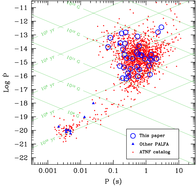
The TOAs from Arecibo and Jodrell Bank (where applicable) were combined into a single data set for each pulsar, which was fit to a standard timing model using $\chi^{2}$ minimization techniques implemented in the Tempo software package. The basic timing model for each source was parameterized by right ascension, $\alpha$; declination, $\delta$; pulse phase; rotation period, $P$; rotation period time derivative, $\dot{P}$; and dispersion measure, DM. Additional parameters were fit to model timing noise in some pulsars, and a glitch in one pulsar, as described below. The best-fit parameters for each pulsar are listed in Table 1. Parameter uncertainties listed in the table are twice the formal uncertainties calculated in the timing model fit. Spin periods and period derivatives are plotted in Figure 1. Values of DM given in this table do not include corrections for scattering or intrinsic profile evolution (Section 6.2).

For pulsars observed at Jodrell Bank, an arbitrary time offset was allowed between the Arecibo and Jodrell Bank TOAs. The timing analysis used the JPL DE405 solar system ephemeris (Standish, 1998) and the TT(BIPM11) time scale. Because of the prevalence of timing noise (see below), unweighted fits were used.

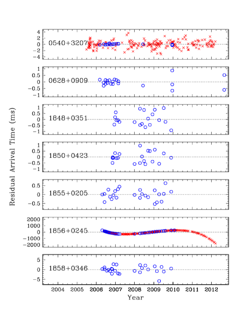
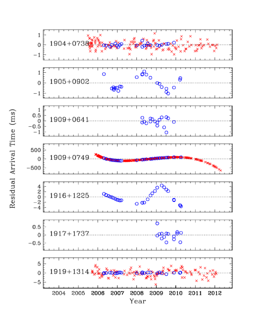
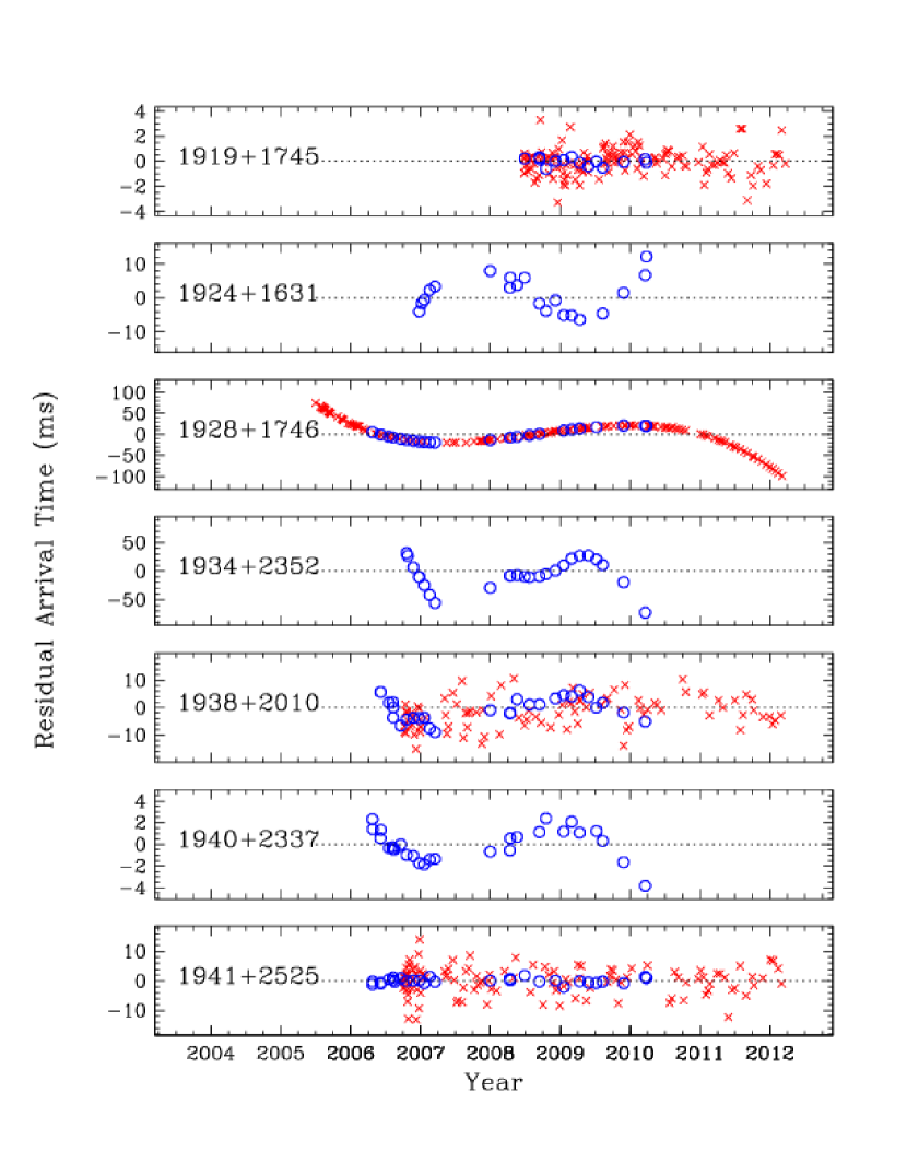
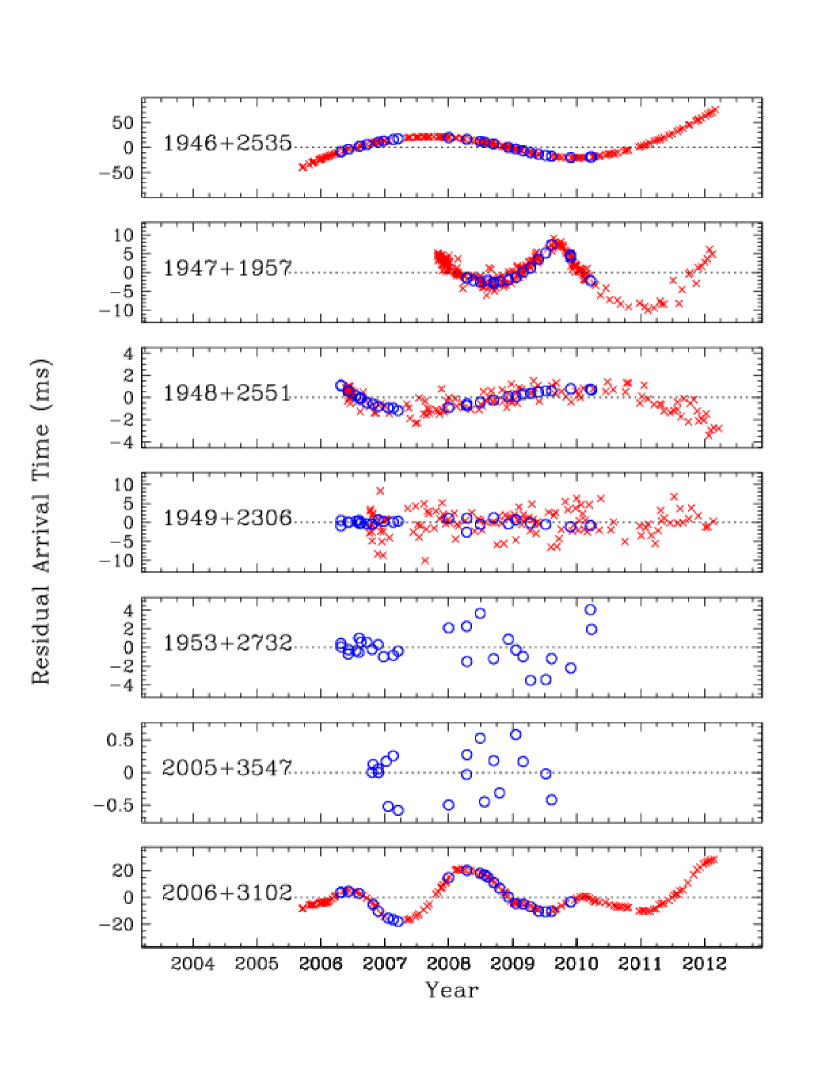
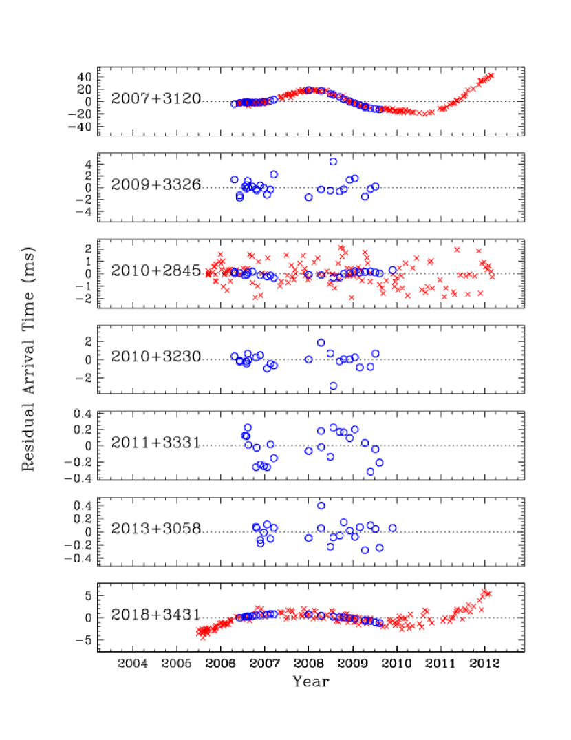
Residual pulse arrival times from fits of each pulsar to the basic timing model are shown in Figures 2(a)-(e). Timing noise is evident in many sources. To measure accurate pulsar parameters, TOAs for these sources were “whitened” by including Taylor expansionss of the pulsar periods in the timing models, $P(t)=\sum_{n=0}^{n_{\rm fit}}(1/n!)P^{(n)}(t-t_{0})^{n}$, where $t$ is the time, $t_{0}$ is the period epoch, and $P^{(n)}\equiv[d^{n}P/dt^{n}]_{t_{0}}$. For each pulsar, models with $n_{\rm fit}$ from 1 (the basic timing model) through 10 were tried, and an appropriate value of $n_{\rm fit}$ was chosen based on the standard deviations of the residuals and on visual inspection of the residuals to ensure there were not groups of correlated nonzero residuals. The chosen values of $n_{\rm fit}$ for each pulsar are listed in Table 1.

For four pulsars, designated as “N” in the $n_{\rm fit}$ column of Table 1, polynomial models with $n_{\rm fit}$ as high as 10 did not yield white residuals. An alternative method was used to estimate the value of each timing parameter for these pulsars. For each pulsar, the timing model (including 10th-order polynomial in $P(t))$ which minimized $\chi^{2}$ was found. Each parameter was then individually perturbed (allowing other parameters to freely vary in the fit) to find the parameter values which resulted in a threefold increase in the standard deviation of the residuals. The resulting range of parameter values was used to set the uncertainties presented in Table 1. We view this as a highly conservative approach to estimating the uncertainties.

Because many of the pulse periods were analyzed as high-order Taylor series around the period epochs, the values of $P$ and $\dot{P}$ listed in Table 1 are the best estimates of the values at the period epoch; they are not averages over the length of the data set.

In Table 2 we present several quantities derived from the timing model parameters. Estimates of spin-down age, $t_{\rm s}$, surface magnetic field strength, $B$, and spin-down energy loss rates, $\dot{E}$, were made using conventional formulae (Lorimer & Kramer, 2005) and are given in logarithmic form in the table. Positions in Galactic coordinates are based on the positions in equatorial coordinates in Table 3. Distances are estimated from dispersion measured in Table 1 using the NE2001 model of the distribution of ionized material in the Galaxy (Cordes & Lazio, 2002). The positions of the pulsars projected onto the Galactic plane are shown in Figure 3.

We detected one glitch, in PSR J1947+1957, as evinced by the peak in the residual pulse arrival times for this pulsar in Figure 2(d). The glitch event was on MJD $55085.5\pm 2.6$ and was well fit by an instantaneous, permanent change in rotation frequency of $\Delta\nu=(1.02\pm 0.03)\times 10^{-8}\,{\rm s}^{-1}$, which is a fractional change of $\Delta\nu/\nu=(1.61\pm 0.04)\times 10^{-9}$. This is a typical value for a small pulsar glitch (e.g., Espinoza et al., 2011). Other pulsars in our data set may have had glitch-like events; in particular, see the residual arrival times of PSRs J1905+0902 and J1916+12245 in Figure 2(b). However, due to the small sizes of the events and the coarse sampling of the time series, these events cannot easily be distinguished from smoothly-varying timing noise.

5. Fluxes and spectral indices

Flux densities and spectral indices of the pulsars are given in Table 4. These were measured from the calibrated pulse profiles from the Arecibo observations by the following procedure. (For logistical reasons, only data from some observing dates were used.) Each profile was generated from a 30 s observation in one of the four 100 MHz subbands, as described above. The flux density was measured in each profile. All flux density measurements for a given subband in a given day were combined; the resulting daily average values were then combined to find a global average for that subband. Finally, the four average flux densities from the four subbands were fit to a function of the form $S(f)=S_{1400}(f_{\rm MHz}/1400)^{\alpha}$, with flux density $S_{1400}$ and spectral index $\alpha$ as free parameters in the fit. The best-fit parameters for each pulsar are given in Table 4, along with the reduced chi-squared values, $\chi^{2}_{\nu}$, of the fits. Although the formal uncertainties from the fits are reported in the table, they should be interpreted with caution, both because they arise from fits with only two degrees of freedom (four data points and two fit parameters) and because scintillation could cause apparent, non-intrinsic variations in pulsar flux densities from epoch to epoch. Table 4 also includes luminosity estimates, $L_{1400}=S_{1400}d^{2}$, using the distances derived from DMs as reported in Table 3.

6. Profile morphologies and scattering properties

6.1. Profiles

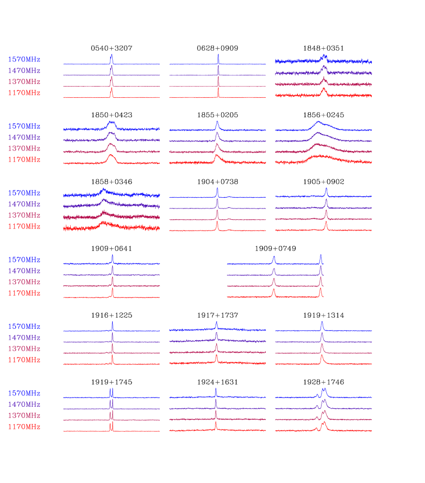
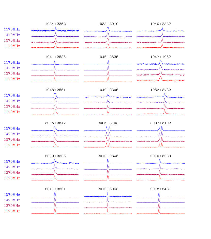
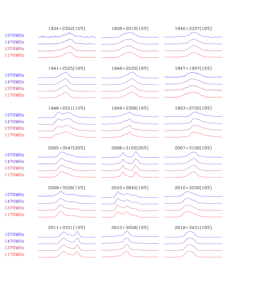
Profiles of each pulsar in each of the four observing subbands are given in Figures 4–5. These average profiles were generated by coherently adding all Arecibo data profiles for a given pulsar that yielded good TOAs. The alignment of the profiles was made using the timing solutions described in Section 4. By and large, these profiles are typical of those seen in the previously known pulsar population. Some evidence of profile evolution over frequency is seen (e.g., relative component strengths of PSR J1948+2551).

One source, J1909+0749, has a strong interpulse. Of its two pulse components, we have somewhat arbitrarily designated the shorter, broader component (near the center of its profiles in Figure 4(a)) as the main pulse and the taller, narrower component (near the end of its profiles in Figure 4(a)) as the interpulse. The interpulse trails the main pulse by $\sim 0.484$ of a pulse period (174^∘). The ratio of integrated flux density for the main pulse over that of the interpulse in each of the Arecibo observing subbands is 1.28, 1.21, 1.02, and 1.36, at 1170, 1370, 1470, and 1570 MHz, respectively. We do not know of a physical explanation for the dip in this ratio at 1470 MHz.

The profiles in Figures 4(a) and (b) were used to compute pulse widths at half-maximum, $W_{50}$, for each pulsar in each observing band. The values are given in Table 5, both in milliseconds and as a fraction of a pulse period.

6.2. Scattering

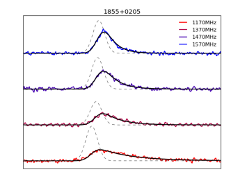
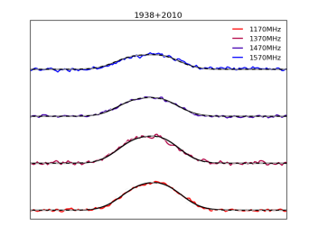
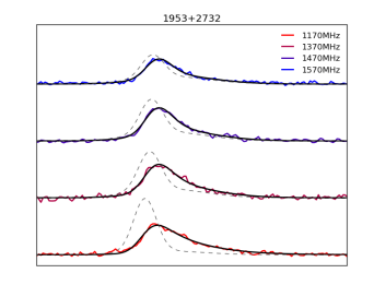
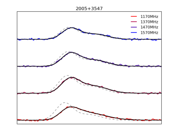
The profiles of several pulsars show evidence of frequency-dependent pulse broadening, indicative of multipath scattering in the interstellar medium. The observed profiles result from the convolution of pulse-broadening functions (PBFs) with the intrinsic pulse shapes. To quantify the scattering for each pulsar’s signal, we used least-squares techniques to simultaneously fit PBFs to the profiles of the pulsar in each of the four observing subbands. While PBFs can take on a range of shapes dependent on the distribution of scattering material along the line of sight and on the wavenumber spectrum of irregularities, for simplicity we adopt a one-sided exponential form with a characteristic $e^{-1}$ broadening time that scales as $\tau_{\rm iss}(f)=\tau_{\rm 1GHz}(f/{\rm 1\,GHz})^{-4}$. We modeled the intrinsic profile of each pulsar as a sum of between one and five Gaussian components. The position and width of each component was held fixed across all four subbands, but the amplitudes were free to vary. The fit included scattering time, $\tau_{\rm 1GHz}$; an arbitrary offset in DM, $\Delta$DM, to account for biases in the DM used to generated the profiles (since the dedispersion used for those profiles did not account for scattering); the position and width of each component; and the amplitude of each component in each subband. Thus, a total of 8–32 parameters were free to vary in the fit for each pulsar, depending on the number of Gaussian components in the model intrinsic profile. Some profiles had noisy baselines, presumably due to radio frequency interference; a polynomial (up to 20th order) was included in the model fit to such profiles.

This model proved satisfactory for all pulsars in our sample. Examples of fitted pulse profiles are in Figure 6. The results of all the fits are given in Table 3, which lists $\tau_{\rm 1GHz}$; $\Delta$DM; the number of components in the profile model, $n_{\rm comp}$; and the goodness-of-fit statistic, $\chi^{2}_{\nu}$. Scattering was detectable in a large number of the sources, and the time scales were determined with precision of a few percent for the most highly scattered sources. The fits are characterized by reduced chi-squared values around $\chi_{\nu}^{2}=1.0\pm 0.5$ for most sources. Even though this method fits the pulse profile well, there is an uncertainty in assuming Gaussian-shaped components in the intrinsic profile models. For a multi-component model combined with a small amount of scattering, the second or third component is covariant with scattering time. We are not able to resolve the ambiguity with the current data. Observations at lower frequency (and hence higher scattering) and measurements of scintillation bandwidths could help resolve these covariances.

We have not tested for departures from the assumed frequency dependence $\tau_{\rm iss}\propto f^{-4}$ or for the dependence of the results on alternative forms for the PBFs, such as those that result from electron-density variations having a Kolmogorov wavenumber spectrum and distributed in a thin screen or an extended medium (Lambert & Rickett, 1999). Anisotropic scattering also presents alternative PBF forms as does any variation of the scattering transverse to the line of sight (Cordes & Lazio, 2001).

A comparison between our measured scattering time scales for pulsars in the inner Galaxy ($30^{\circ}<l<80^{\circ}$) and the predictions of the NE2001 electron-density model (Cordes & Lazio, 2002) is given in Figure 7. The pulse broadening times in our sample of pulsars displays the same amount of variation at a given value of DM as is seen in other objects (e.g., Cordes & Lazio, 2002; Bhat et al., 2004). While the NE2001 electron-density model generally underpredicts the pulse broadening times for the pulsars in our sample with the largest pulse broadening, the broadening times are consistent with the observed ranges from the larger sample of objects used to construct NE2001 and analyzed in Bhat et al. (2004). The underprediction is especially notable for objects in the Cygnus direction (as seen at the higher Galactic longitudes in Figure 7). This is to be expected because the Cygnus superbubble comprises discrete H ii regions that are known to produce excess scattering (Fey et al., 1989).

All but one of the pulsars (PSR J2005+3547) have DMs that can be accommodated by the NE2001 model, but some of the DM values and pulse broadening times are undoubtedly enhanced by intersection of the line of sight with particular electron-density enhancements not included in NE2001. A new electron density model is now under development that will include the DM values and scattering measurements discussed here.

The scattering measurements imply that searches for millisecond pulsars along low-Galactic-latitude lines of sight in our observing region of $32^{\circ}<\ell<77^{\circ}$ will be limited by scattering at very large distances. Presuming a scaling law of $\tau_{\rm iss}\propto f^{-4}$, the median measured value $\tau_{\rm 1GHz}\approx 4\,{\rm ms}$ among our pulsars scales to $\tau_{\rm 1.42GHz}\approx 1\,{\rm ms}$. Scattering of this magnitude significantly curtails sensitivity to the fastest-spinning pulsars, especially those with periods of order 1 ms. (It is important to note that there is still a large volume of space, likely extending to distances of several kiloparsecs, for which scattering is not significant, and within which there is promise for a large number of millisecond pulsars to be detected by surveys such as PALFA.)

7. X-ray Observations of PSR J1856+0245

The 81-ms pulsar J1856+0245 has the smallest characteristic age, 21 kyr, and largest spin-down luminosity, $\dot{E}=4.6\times 10^{36}\,{\rm erg\,s}^{-1}$, of the pulsars observed for this paper. Hessels et al. (2008) found this pulsar to be coincident with the extended TeV source HESS J1857+026 and noted faint X-ray emission in the pulsar’s vicinity in archival ASCA data. They concluded that HESS J1857+026 was plausibly a pulsar wind nebula (PWN) associated with PSR J1856+0245. Rousseau et al. (2012) examined 36 months of Fermi Large Area Telescope $\gamma$-ray data toward this pulsar. They detected emission coincident with the pulsar and extended TeV source, but they did not detect pulsations. They interpreted the unpulsed emission from the region as a putative GeV PWN, and performed multi-wavelength (keV–TeV) modeling of the spectral energy distribution. Here we describe dedicated XMM-Newton and Chandra X-ray observations of this region, which were obtained to verify the PWN interpretation. These observations were used in Rousseau et al. (2012) to place a limit on the flux of any extended X-ray emission. We present for the first time the X-ray spectrum of the pulsar and further discuss its association with the GeV–TeV emission.

7.1. XMM-Newton

XMM-Newton observed the field of PSR J1856+0245 on 2008 March 27–28 (ObsID 0505920101) for a total of 55.3 ks. Data were acquired from only the European Photon Imaging Camera (EPIC) pn detector, operating in full-frame imaging mode with the thick optical filter in place. Unfortunately, due to tests being conducted simultaneously on the MOS1 and MOS2 detectors, no data are available from those instruments. The EPIC pn field of view was centered close to the timing position of PSR J1856+0245 and also included the centroid of the TeV nebula HESS J1857+026 (Figure 8). The raw (ODF) pn data were reprocessed using the Epchain pipeline in SAS. The data were subsequently screened for instances of strong soft-proton flaring. The filtering procedure left 30.2 ks of useful exposure time. The Reflection Grating Spectrometer data provided no useful source information and are not included in our analysis. The SAS source detection task edetect_chain found a source coincident with the radio timing position of PSR J1856+0245, XMMU J185650.8+024545.

Photons were extracted from a circular region of radius $10^{\prime\prime}$ centered on the pulsar, which encloses $\sim$52% of the total energy. This relatively small extraction radius was chosen to minimize contamination from the nearby ($\sim 22^{\prime\prime}$) source XMMU J185651.8+024530. An estimate of the background was obtained from several source-free regions around the pulsar position. The spectral analysis was performed using Xspec 12.5.0.5. The source spectrum was grouped to ensure at least 15 photons per energy bin.

The X-ray counterpart of PSR J1856+0245 shows a hard spectrum, most likely because it is distant and heavily absorbed. We fit the spectrum of the source with both absorbed power-law and thermal models. Given the low photon count, both models describe the data adequately well, though an absorbed blackbody model gives a temperature of $kT\approx 1.5-3\,{\rm keV}$, too hot to be the surface temperature of the neutron star. For this reason, the power law model is preferred. For young pulsars, such emission is typically due to particle acceleration in the pulsar magnetosphere. The best-fit parameters for this model are only weakly constrained due to the limited number of photons with absorption $N_{\rm H}=(4.9^{+3.2}_{-2.4})\times 10^{22}\,{\rm cm}^{-2}$ and photon index $\Gamma=1.2^{+0.8}_{-0.4}$. The implied unabsorbed flux is $\sim$$8.3\times 10^{-14}$ erg cm^-2 s^-1 (2–10 keV), which for a distance of $9$ kpc (Table 3) corresponds to a luminosity of $L_{X}\sim 8\times 10^{32}$ erg s^-1.

The 73.4 ms time resolution of the EPIC pn full-frame exposure and the 3.2 s frame time of the ACIS-I observation preclude the search for X-ray pulsations from PSR J1856+0245.

7.2. Chandra

PSR J1856+0245 was observed with Chandra ACIS-I for 39 ks on 2011 February 28 (ObsID 12557). These data were recorded in VFAINT and Timed Exposure modes and were analyzed using CIAO version 4.3.1 with CALDB 4.4.3. PSR J1856+0245 is clearly detected as a point source (Figure 8). As also discussed in Rousseau et al. (2012), there is no evidence for extended emission surrounding the pulsar. Subtracting a simulated point spread function using ChaRT and marx from the observed point source yields no excess counts that could arise due to a compact PWN. Extracting the emission from an annular region with inner and outer radii of 2^′′ and 15^′′, respectively, we find an upper limit on the unabsorbed flux of $5\times 10^{14}$ erg s^-1 cm^-2 (1–10 keV, 3$\sigma$ confidence), corresponding to a luminosity of $\lesssim$$5\times 10^{32}$ erg s^-1. In deriving this limit we assumed a power-law index of $\Gamma=1.5$ and an equivalent neutral hydrogen column depth $N_{\rm H}=4\times 10^{22}\,{\rm cm}^{-2}$. The latter is somewhat higher than would be predicted by a simple empirical correlation between $N_{\rm H}$ and DM (He et al., 2013), so can be regarded as conservative. Note that the outer extraction radius was chosen based on the X-ray PWN for pulsars with comparable $\dot{E}$ by scaling their angular size with the distance (Kargaltsev & Pavlov, 2008), assuming a distance of 9 kpc (Table 3).

7.3. Association between PSR J1856+0245 and HESS J1857+026

Hessels et al. (2008) showed that PSR J1856+0245 is coincident with the faint ASCA X-ray source AX J185651+0245 and suggested that the latter might represent an X-ray PWN associated with the pulsar. Our XMM-Newton and Chandra observations confirm X-ray emission from the pulsar itself, but find no evidence of surrounding diffuse emission. While the discovery of an X-ray PWN—especially one which shows a morphology indicative of an association with the TeV PWN (e.g., Aharonian et al., 2005)—would strengthen the link between PSR J1856+0245 and HESS J1857+026, the lack of an observable X-ray PWN does not eliminate the possibility of association. Given the distance of 9 kpc inferred from the pulsar’s DM, it is possible that the X-ray PWN is simply too faint to be detected in the current data. Indeed, Rousseau et al. (2012) show that it is possible to derive a self-consistent model of the spectral energy distribution that accounts for the low X-ray nebula flux.

We have taken a critical look at other X-ray sources detected in our XMM-Newton and Chandra observations, and find no evidence for extended sources of a possible PWN nature (Figure 8). These observations do not cover the full extent of the TeV nebula, but they do include the source centroid. Furthermore, the PALFA survey has covered the region of the HESS TeV emission and as such any additional, undiscovered, young pulsar in the region would have to be quite faint, $S_{1400}\lesssim 0.2$ mJy (depending on the duty cycle, DM, and scattering). We thus conclude that PSR J1856+0245 remains the most viable association for HESS J1857+026.

8. Discussion

We have presented timing properties and pulsar profile morphologies of 35 pulsars discovered in the PALFA survey. Due to this survey’s depth and its sensitivity to high-DM pulsars, these pulsars are relatively distant, with a median distance of 7.1 kpc compared to the median distance of 4.2 kpc of Galactic pulsars listed in the ATNF pulsar catalog (Figure 3 and Table 3).

Despite their large distances, the properties of these pulsars are similar to those of the previously known non-recycled Galactic pulsar population. We used Kolmogorov-Smirnov tests to compare the distributions of spin-down ages, magnetic field strengths, and spin-down energies of the pulsars in this paper with those of the known pulsar population. We excluded recycled pulsars from this comparison by imposing a cutoff $\dot{P}>10^{-17}$. We found no significant differences between the two populations. (A more thorough analysis of the population of pulsars discovered by PALFA, using more powerful statistical techniques and considering the details of the telescope search pointings, is beyond the scope of the present paper.)

Four of the sources, PSRs J1856+0245, J1909+0749, J1928+1746 and J1934+2352, have spin-down ages $t_{s}<10^{5}$ yr. Pulsars of such young age are often found in supernova remnants. However, Green’s Supernova Remnant catalog (Green, 2009) lists no remnants coincident with the positions of these pulsars. The remnant catalog is known to be incomplete, however, and dedicated radio interferometric observations of these objects in particular to look for remnants could be fruitful.

Young and energetic radio pulsars often have counterparts at other wavelengths, such as the X-ray source at the position of PSR J1856+0245 described above. We have checked the ROSAT all-sky survey for X-ray point sources at the positions of all the pulsars having $\dot{E}>2\times 10^{35}$ erg s^-1, but we have found no counterparts.

As discussed in Section 4, many of the pulsars in this paper show deviations from steady spin-down (Figures 2(a)–(e)). The spin evolution of a pulsar is conventionally quantified by a braking index, $n$, defined through $\dot{\nu}\propto\nu^{n}$, where $\nu=1/P$ is the spin frequency and $\dot{\nu}$ is its time derivative. For a pulsar undergoing energy loss due to magnetic dipole rotation, $n=3$. In principle, the braking index for a pulsar can be calculated from $n=\nu\ddot{\nu}/\dot{\nu}^{2}$ if the second time derivative of spin frequency, $\ddot{\nu}$, is known (Lorimer & Kramer, 2005). In practice, such measurements have been achieved for only a few pulsars (e.g., Livingstone et al., 2005, and references therein). Most measurements of $\ddot{\nu}$ and inferred values of $n$ have been much larger in magnitude than predicted by steady spin-down models. Hobbs et al. (2010) analyzed long-term pulsar timing data of hundreds of pulsars and found that pulsars with spin-down ages less than $10^{5}$ yr all had positive values of $n$, whereas older pulsars had a mix of positive and negative values. They interpreted this as evidence that young pulsars are recovering from glitches that occurred prior to the starts of the data sets, while older pulsars are dominated by stochastic processes.

Significant values of $\ddot{\nu}$, and hence $n$, can be measured for about half of our sources (all those for which $n_{\rm fit}>1$ in Table 1). The four pulsars with spin-down ages less than $10^{5}$ yr all show positive values of $n$: $n=24.5,11.3,22.9,{\rm and}\ 12.3$ for PSRs J1856+0245, J1909+0749, J1928+1746, and J1934+2352, respectively, consistent with the findings of Hobbs et al. (2010). The older pulsars show a mix of positive and negative values of $n$. All measured values of $n$ are sufficiently large in magnitude to suggest that they are not associated with steady spin-down of these pulsars.

The dispersion measurements and scattering measurements presented in Sections 4 and 6.2 are a promising start of the detailed study of the ionized interstellar medium in this range of Galactic longitudes. The scattering measurements could be greatly enhanced by collecting and analyzing profiles of these sources at longer wavelengths.

The 35 pulsars in this paper are just the tip of the iceberg. As of this writing, the ongoing PALFA survey had discovered more than 100 pulsars. Study of these objects will enhance our knowledge of the pulsar population and the interstellar medium in this sector of the Galaxy.

Table 1Timing Parameters of 35 Pulsars

PSR	Previous	$\alpha$	$\delta$	Epoch of $P$	$P$	$\dot{P}$	DM	$n_{\rm fit}$
	Reference	(J2000)	(J2000)	(MJD)	(s)	($10^{-15}$)	(pc cm-3)
J0540+3207	1	05:40:37.116(1)	32:07:37.3(1)	54780.000	0.5242708632083(5)	000.44811(2)	0061.97(4)	1
J0628+0909	1,2	06:28:36.183(5)	09:09:13.9(3)	54990.000	1.241421391299(3)	000.5479(2)	0088.3(2)	1
J1848+0351		18:48:42.24(1)	03:51:35.7(3)	54620.000	0.191442663494(2)	000.0673(1)	00336.6(4)	1
J1850+0423		18:50:23.43(1)	04:23:09.2(4)	54600.000	0.290716217162(3)	000.0914(2)	00265.8(4)	1
J1855+0205		18:55:42.046(5)	02:05:36.4(2)	54510.000	0.2468167699732(9)	000.06466(7)	00867.3(2)	1
J1856+0245	3	18:56:50.9(3)	02:45:47(9)	54930.000	0.08090668906(4)	0062.117(4)	00623.5(2)	N
J1858+0346		18:58:22.36(2)	03:46:37.8(8)	54510.000	0.256843797950(5)	002.0401(4)	00386(1)	1
J1904+0738	1	19:04:07.533(1)	07:38:51.69(4)	54760.000	0.2089583321216(2)	000.410898(7)	00278.32(8)	1
J1905+0902	1	19:05:19.535(2)	09:02:32.49(8)	54570.000	0.2182529126846(9)	003.49853(8)	00433.4(1)	3
J1909+0641	2	19:09:29.052(4)	06:41:25.8(2)	54870.000	0.741761952452(6)	003.2239(7)	0036.7(2)	1
J1909+0749		19:09:08.2(2)	07:49:32(5)	54870.000	0.23716129322(9)	00151.920(9)	00539.36(5)	N
J1916+1225		19:16:20.045(1)	12:25:53.94(4)	54570.000	0.227387488792(2)	0023.4516(2)	00265.31(3)	8
J1917+1737		19:17:23.976(5)	17:37:31.6(1)	55070.000	0.334725226760(4)	000.324(1)	00208.0(2)	1
J1919+1314		19:19:32.986(5)	13:14:37.3(1)	54790.000	0.571399860595(2)	003.78771(6)	00613.4(2)	1
J1919+1745	2	19:19:43.342(4)	17:45:03.79(8)	55320.000	2.081343459724(9)	001.7050(4)	00142.3(2)	1
J1924+1631		19:24:54.88(3)	16:31:48.8(6)	54690.000	2.9351864592(2)	00364.212(4)	00518.5(9)	2
J1928+1746	1	19:28:42.553(1)	17:46:29.62(3)	54770.000	0.0687304058253(2)	0013.190700(6)	00176.68(5)	4
J1934+2352		19:34:46.19(2)	23:52:55.9(3)	54650.000	0.17843152366(2)	00130.699(2)	00355.5(2)	8
J1938+2010		19:38:08.34(2)	20:10:51.7(4)	54940.000	0.68708185664(2)	003.399(1)	00327.7(8)	4
J1940+2337		19:40:35.486(7)	23:37:46.5(2)	54560.000	0.546824157964(7)	0076.7965(2)	00252.1(3)	2
J1941+2525		19:41:20.80(1)	25:25:05.3(2)	54920.000	2.30615269700(2)	00160.8349(5)	00314.4(4)	1
J1946+2535		19:46:49.10(5)	25:35:51.5(9)	54810.000	0.51516705131(6)	005.641(5)	00248.81(4)	N
J1947+1957		19:47:19.435(4)	19:57:08.39(9)	55190.000	0.157508542541(4)	000.5226(1)	00185.8(2)	1
J1948+2551		19:48:17.579(1)	25:51:51.95(2)	54930.000	0.1966268136138(4)	009.02244(2)	00289.27(5)	3
J1949+2306		19:49:07.32(1)	23:06:55.5(2)	54910.000	1.31937338530(1)	000.1231(3)	00196.3(5)	1
J1953+2732		19:53:07.80(2)	27:32:48.2(4)	54570.000	1.33396499366(2)	001.773(1)	00195.4(9)	1
J2005+3547		20:05:17.493(9)	35:47:25.4(1)	54540.000	0.615033894871(4)	000.2808(3)	00401.6(3)	1
J2006+3102		20:06:11.0(3)	31:02:03(4)	54800.000	0.16369523645(9)	0024.872(9)	00107.16(1)	N
J2007+3120		20:07:09.012(6)	31:20:51.54(9)	54920.000	0.60820531457(1)	0015.604(1)	00191.5(2)	9
J2009+3326	1	20:09:49.16(2)	33:26:10.2(3)	54430.000	1.43836860189(2)	001.468(2)	00263.6(8)	1
J2010+2845		20:10:05.068(2)	28:45:29.17(3)	54810.000	0.5653693451984(6)	000.09072(2)	00112.47(8)	1
J2010+3230	1	20:10:26.50(1)	32:30:07.3(2)	54430.000	1.44244752060(1)	003.616(1)	00371.8(5)	1
J2011+3331	1	20:11:04.926(2)	33:31:24.64(3)	54490.000	0.931733093470(4)	001.7857(1)	00298.58(6)	2
J2013+3058		20:13:34.253(3)	30:58:50.69(5)	54600.000	0.2760276934460(5)	000.15194(4)	00148.7(1)	1
J2018+3431	1	20:18:53.196(2)	34:31:00.51(2)	54760.000	0.3876640866385(8)	001.83649(2)	00222.35(7)	2

Table 2Quantities Derived from Rotation Parameters of Table 1.

PSR	$\log\,t_{\rm s}$	$\log\,B$	$\log\,\dot{E}$
	(log yr)	(log G)	(log erg s-1)
J0540+3207	7.27	11.7	32.1
J0628+0909	7.56	11.9	31.0
J1848+0351	7.65	11.1	32.6
J1850+0423	7.70	11.2	32.2
J1855+0205	7.78	11.1	32.2
J1856+0245	4.31	12.4	36.7
J1858+0346	6.30	11.9	33.7
J1904+0738	6.91	11.5	33.2
J1905+0902	5.99	11.9	34.1
J1909+0641	6.56	12.2	32.5
J1909+0749	4.39	12.8	35.6
J1916+1225	5.19	12.4	34.9
J1917+1737	7.21	11.5	32.5
J1919+1314	6.38	12.2	32.9
J1919+1745	7.29	12.3	30.9
J1924+1631	5.11	13.5	32.7
J1928+1746	4.92	12.0	36.2
J1934+2352	4.34	12.7	36.0
J1938+2010	6.51	12.2	32.6
J1940+2337	5.05	12.8	34.3
J1941+2525	5.36	13.3	32.7
J1946+2535	6.16	12.2	33.2
J1947+1957	6.68	11.5	33.7
J1948+2551	5.54	12.1	34.7
J1949+2306	8.23	11.6	30.3
J1953+2732	7.08	12.2	31.5
J2005+3547	7.54	11.6	31.7
J2006+3102	5.02	12.3	35.3
J2007+3120	5.79	12.5	33.4
J2009+3326	7.19	12.2	31.3
J2010+2845	7.99	11.4	31.3
J2010+3230	6.80	12.4	31.7
J2011+3331	6.92	12.1	31.9
J2013+3058	7.46	11.3	32.4
J2018+3431	6.52	11.9	33.1

Table 3Galactic Positions, Distance, and Scattering Properties.

					NE2001 Predictions			Measured Values
PSR	$l$	$b$	DM		$d$	$\tau_{\rm 1GHz}$		$\tau_{\rm 1GHz}$	$\Delta$DM	$n_{\rm comp}$	$\chi^{2}_{\nu}$
	$(^{\circ})$	$(^{\circ})$	(pc cm-3)		(kpc)	(ms)		(ms)	(pc cm-3)
J1924+1631	51.405	$0.318$	518.5		$>$14.0	00.50		49(2).00	0$-10.4(8)$00	2	1.3
J1858+0346	37.084	$0.182$	386.6		$>$07.0	04.97		42(3).00	0$-3.0(4)$00	3	1.1
J2010+3230	70.391	$-0.495$	371.8		$>$12.0	00.08		24.8(6)0	0$-3.8(1)$00	1	1.0
J1953+2732	64.205	$0.059$	195.4		$>$07.0	00.01		21(3).00	0$-2.8(2)$00	3	1.1
J1919+1314	47.895	$-0.088$	613.5		$>$15.2	01.87		18.7(9)0	0$-2.11(5)$0	2	1.5
J1856+0245	36.008	$0.057$	623.5		$>$09.0	23.31		18.0(6)0	0$-3.0(1)$00	2	1.0
J1855+0205	35.281	$0.007$	867.3		$>$11.6	57.33		16.3(9)0	0$-2.1(1)$00	2	1.4
J2005+3547	72.581	$2.180$	401.7		$>$50.0	00.07		11(1).00	0$-1.85(9)$0	2	1.5
J1850+0423	36.718	$2.231$	265.9		$>$06.4	00.28		07.8(8)0	+0$0.0(2)$00	2	1.3
J1941+2525	61.037	$1.263$	314.4		$>$09.8	00.03		07.4(6)0	0$-2.4(2)$00	2	1.5
J1948+2551	62.207	$0.131$	289.3		$>$08.8	00.02		06.3(2)0	0$-0.83(1)$0	4	1.5
J1949+2306	59.931	$-1.423$	196.4		$>$07.0	00.01		05.4(7)0	0$-1.0(1)$00	3	1.4
J1916+1225	46.811	$0.225$	265.3		$>$07.1	00.59		05.3(2)0	0$-0.155(9)$	4	1.6
J1946+2535	61.809	$0.283$	248.8		$>$08.1	00.01		04.54(7)	0$-0.97(2)$0	3	1.8
J1938+2010	56.115	$-0.672$	327.7		$>$09.5	00.05		04(1).00	+0$0.1(4)$00	2	1.1
J2011+3331	71.320	$-0.049$	298.6		$>$08.8	04.16		04.39(9)	0$-0.84(2)$0	3	1.9
J1940+2337	59.397	$0.529$	252.2		$>$08.2	00.02		04.2(5)0	0$-0.8(1)$00	2	1.3
J2007+3120	69.042	$-0.535$	191.6		$>$06.8	00.01		03.8(8)0	0$-0.52(6)$0	2	1.6
J1919+1745	51.897	$1.987$	142.3		$>$05.2	00.01		02.9(2)0	0$-0.60(5)$0	4	1.8
J1909+0749	41.909	$-0.340$	539.4		$>$09.5	06.31		01.9(1)0	0$-0.32(4)$0	5	1.5
J1904+0738	41.180	$0.680$	278.3		$>$06.3	01.01		01.61(7)	0$-0.30(2)$0	3	1.4
J2018+3431	73.044	$-0.841$	222.3		$>$07.2	00.02		01.2(1)0	0$-0.35(3)$0	2	1.3
J1905+0902	42.555	$1.056$	433.5		$>$09.1	01.78		00.9(2)0	0$-0.22(6)$0	3	1.6
J2013+3058	69.485	$-1.886$	148.8		$>$06.0	00.00		$<$0.9000)	0$-0.10(6)$0	3	1.6
J1917+1737	51.528	$2.418$	208.1		$>$07.0	00.02		$<$1.0000)	0$-0.1(3)$00	2	1.2
J1928+1746	52.931	$0.114$	176.7		$>$05.8	00.04		$<$0.6000)	0$-0.11(4)$0	5	1.3
J1848+0351	36.058	$2.366$	336.7		$>$07.9	00.41		$<$1.0000)	+0$0(1)$.000	1	1.5
J2006+3102	68.667	$-0.530$	107.2		$>$04.7	00.00		$<$1.0000)	+0$0.03(6)$0	5	1.4
J2009+3326	71.103	$0.124$	263.6		$>$07.9	01.73		$<$1.0000)	+0$0.1(1)$00	3	1.3
J1934+2352	58.966	$1.814$	355.5		$>$11.6	00.03		$<$1.0000)	+0$0.1(2)$00	2	1.6
J2010+2845	67.210	$-2.472$	112.5		$>$05.0	00.00		$<$1.0000)	0$-0.07(3)$0	3	3.5
J1909+0641	40.941	$-0.940$	36.7		$>$02.2	00.00		$<$1.0000)	+0$0.00(3)$0	3	1.6
J0540+3207	176.719	$0.761$	62.0		$>$01.8	00.00		$<$1.0000)	0$-0.060(5)$	2	2.6
J0628+0909	202.190	$-0.851$	88.3		$>$02.5	00.00		$<$1.0000)	+0$0.144(9)$	1	3.7
J1947+1957	56.987	$-2.658$	185.9		$>$06.8	00.01		$<$1.0000)	0$-0.03(4)$0	2	1.5

Table 4 Flux Densities, Spectral Indices, and Luminosities.

PSR	$S_{1400}$	$\alpha$	$\chi^{2}_{\nu}$	$L_{1400}$
	(mJy)			(Jy kpc2)
J0540+3207	0.34(2)	$-2.0(3)$	0.384	1.1
J0628+0909	0.058(3)	$-0.7(5)$	0.571	0.4
J1848+0351	0.066(2)	$-2.1(4)$	0.665	4.1
J1850+0423	0.199(4)	$-2.9(2)$	0.687	8.1
J1855+0205	0.193(5)	$-1.4(3)$	1.313	24.5
J1856+0245	0.58(2)	$-0.4(2)$	10.602	45.5
J1858+0346	0.190(9)	$-3.0(4)$	0.494	10.2
J1904+0738	0.23(1)	$-1.1(4)$	0.029	9.1
J1905+0902	0.097(6)	$-1.7(5)$	0.263	8.5
J1909+0641	0.111(3)	$-1.9(2)$	1.362	0.5
J1909+0749	0.226(8)	$-1.3(3)$	0.098	1.0
J1916+1225	0.094(2)	$-0.6(2)$	1.863	4.4
J1917+1737	0.047(1)	$-1.4(4)$	0.004	2.3
J1919+1745	0.190(8)	$-2.6(4)$	0.174	5.5
J1919+1314	0.224(6)	$-1.3(3)$	2.378	53.9
J1924+1631	0.088(4)	$-0.9(3)$	3.794	17.6
J1928+1746	0.278(8)	$0.0(3)$	1.866	9.5
J1934+2352	0.062(2)	$-3.4(3)$	1.185	8.4
J1938+2010	0.103(9)	$-1.9(7)$	0.233	8.8
J1940+2337	0.069(4)	$0.1(7)$	1.911	5.0
J1941+2525	0.240(8)	$-0.8(3)$	0.097	22.6
J1946+2535	0.480(7)	$-1.6(2)$	4.376	30.9
J1947+1957	0.081(6)	$-1.5(8)$	0.027	3.4
J1948+2551	0.622(7)	$-0.7(1)$	5.619	47.9
J1949+2306	0.097(4)	$-3.3(3)$	1.089	7.8
J1953+2732	0.106(7)	$-3.0(6)$	0.748	9.5
J2005+3547	0.252(9)	$-2.2(4)$	0.082
J2006+3102	0.27(1)	$-1.8(4)$	0.157	6.4
J2007+3120	0.123(5)	$-2.9(4)$	0.291	6.1
J2009+3326	0.15(1)	$-4.1(6)$	0.261	19.7
J2010+2845	0.43(2)	$-2.1(3)$	0.373	9.9
J2010+3230	0.118(5)	$-3.5(3)$	0.902	31.6
J2011+3331	0.384(8)	$-2.5(2)$	1.215	32.9
J2013+3058	0.067(5)	$-3.0(7)$	0.253	2.4
J2018+3431	0.247(9)	$-1.2(3)$	0.693	13.1

Table 5Pulse Widths

PSR	$P$ (ms)	$W_{50}$ (ms)					$W_{50}/P$
		1170	1370	1470	1570		1170	1370	1470	1570
		MHz	MHz	MHz	MHz		MHz	MHz	MHz	MHz
0540+3207	524.3	11.0	11.7	12.0	12.4		0.021	0.022	0.023	0.024
0628+0909	1241.4	7.6	7.7	8.0	8.4		0.006	0.006	0.006	0.007
1848+0351	191.4	9.9	9.9	10.3	12.0		0.052	0.052	0.054	0.063
1850+0423	290.7	24.6	24.3	24.7	24.6		0.084	0.084	0.085	0.085
1855+0205	246.8	20.5	9.4	7.6	6.6		0.083	0.038	0.031	0.027
1856+0245	80.9	23.8	17.6	14.6	14.2		0.295	0.218	0.180	0.175
1858+0346	256.8	41.4	33.9	36.7	32.3		0.161	0.132	0.143	0.126
1904+0738	209.0	3.2	3.0	2.9	2.8		0.015	0.014	0.014	0.013
1905+0902	218.3	3.9	3.7	3.9	3.9		0.018	0.017	0.018	0.018
1909+0641	741.8	8.2	7.9	7.9	7.6		0.011	0.011	0.011	0.010
1909+0749M	237.2	5.6	4.7	5.2	5.0		0.024	0.020	0.022	0.021
1909+0749I	237.2	4.0	3.7	3.7	3.4		0.017	0.016	0.016	0.014
1916+1225	227.4	2.0	1.7	1.7	1.6		0.009	0.008	0.007	0.007
1917+1737	334.7	6.1	5.5	5.9	5.7		0.018	0.016	0.018	0.017
1919+1314	571.4	15.6	13.2	11.5	11.6		0.027	0.023	0.020	0.020
1919+1745	2081.3	63.6	62.4	62.4	62.5		0.031	0.030	0.030	0.030
1924+1631	2935.2	35.1	27.1	27.2	24.1		0.012	0.009	0.009	0.008
1928+1746	68.7	3.4	3.5	3.4	3.4		0.050	0.051	0.050	0.049
1934+2352	178.4	4.5	3.7	4.2	3.3		0.025	0.021	0.024	0.018
1938+2010	687.1	24.7	24.5	25.0	24.7		0.036	0.036	0.036	0.036
1940+2337	546.8	10.6	10.4	9.4	10.3		0.019	0.019	0.017	0.019
1941+2525	2306.2	33.5	36.6	35.6	33.4		0.015	0.016	0.015	0.015
1946+2535	515.2	9.5	8.7	8.6	8.5		0.018	0.017	0.017	0.016
1947+1957	157.5	6.9	6.1	6.5	5.9		0.044	0.039	0.041	0.038
1948+2551	196.6	9.1	9.0	9.2	9.0		0.046	0.046	0.047	0.046
1949+2306	1319.4	17.8	17.8	19.6	21.5		0.013	0.014	0.015	0.016
1953+2732	1334.0	29.7	29.0	26.3	26.7		0.022	0.022	0.020	0.020
2005+3547	615.0	23.3	19.6	20.8	18.9		0.038	0.032	0.034	0.031
2006+3102	163.7	12.2	11.8	11.8	11.8		0.074	0.072	0.072	0.072
2007+3120	608.2	8.7	8.9	8.7	8.8		0.014	0.015	0.014	0.015
2009+3326	1438.4	24.5	25.8	26.7	29.7		0.017	0.018	0.019	0.021
2010+2845	565.4	14.6	14.1	13.6	13.5		0.026	0.025	0.024	0.024
2010+3230	1442.4	30.6	28.1	28.8	26.8		0.021	0.019	0.020	0.019
2011+3331	931.7	30.7	30.6	30.6	30.1		0.033	0.033	0.033	0.032
2013+3058	276.0	3.0	2.8	2.9	3.0		0.011	0.010	0.010	0.011
2018+3431	387.7	6.8	6.6	6.7	6.5		0.017	0.017	0.017	0.017

Figure 1.— Pulsar rotation periods and period derivatives. Blue circles indicate pulsars in the present paper, blue triangles indicate other published pulsars discovered in the PALFA survey, and red dots are all known pulsars in the Galactic disk (Hobbs & Manchester, 2013).

Figure 2.— Part (a). Residual pulse arrival times of all pulsars in this paper are given in (a)-(e). The points are daily average residuals at Arecibo (blue circles) and Jodrell Bank (red $\times$’s). For each pulsar, the residual plot was made by performing a timing fit, possibly including whitening and glitch parameters as described in the text, to find the best-fit parameters; freezing the position at its best-fit value; removing whitening and glitches from the model; re-fitting for spin period and spin-down rate; and averaging the resulting residual pulse arrival times within each day at each observatory.

Figure 2.— Part (b).

Figure 2.— Part (c).

Figure 2.— Part (d).

Figure 2.— Part (e).

Figure 3.— Pulsar positions projected onto the Galactic plane. Pulsar positions are based on the coordinates and distances given in Table 3. The position of the Sun is indicated by a small circle and dot at $(x,y)=(0,8.5\,{\rm kpc})$. Straight lines emerging from the Sun indicate regions of low Galactic latitude within the declination range of the Arecibo telescope. Curved lines indicate Galactic spiral arms according to the NE2001 electron density model (Cordes & Lazio, 2002)). Blue circles indicate pulsars in the present paper; blue triangles indicate other published pulsars discovered in the PALFA survey; and red dots are all known pulsars in the Galactic disk (Hobbs & Manchester, 2013).

Figure 4.— Part (a). Profiles of the pulsars in each of the four observational subbands are given in (a) and (b). Each profile is a full pulse period. Profiles are sums of all Arecibo data records which produced valid TOAs for a given pulsar at a given frequency. Data records were aligned using the final timing solution for each pulsar. Plots are total intensity (summed polarizations). See Figures 5(a) and (b) for expanded views of the pulse peaks.

Figure 4.— Part (b).

Figure 5.— Part (a). Close-up of the pulse peak of each pulse profile in Figures 4(a) and (b). The horizontal range varies from pulsar to pulsar depending on the pulse width and is given above each set of profiles, e.g., “0540+3207(10%)” means that the horizontal extent of the profiles of 0540+3207 is 10% of the pulse period. Two plots are shown for 1909+0749, labeled by “M” and “I,” for main pulse and interpulse; these correspond to the leading (“M”) and trailing components (“I”) of the profile shown in Figure 4(a). These two components are similar in total energy, and the designation of “M” and “I” is arbitrary. They are plotted on the same vertical scale, and the centers of the two plots are separated by half a pulse period.

Figure 5.— Part(b).

Figure 6.— Sample pulsar scattering model fits. Top: PSR J1848+0351, PSR J1855+0205; middle: PSR J1938+2010, PSR J1948+2551; bottom: PSR J1953+2732, PSR J2005+3557. For each pulsar, closeups of the pulse peak are shown for the four observing subbands (top to bottom: 1570, 1470, 1370, and 1170 MHz). Superimposed on each profile are the profile models for that frequency both with scattering (black line) and without scattering (gray line). Of the pulsars shown here, J1855+0205 and J1953+2732 show strong scattering; J1848+0351 and J1938+2010 show almost no scattering; and J1948+2551 and J2005+3547 have high covariance between the Gaussian profile model and the scattering tail.

Figure 7.— Scattering time scales of the pulsars, comparing our measured time scales with the predictions of the NE2001 electron density model (Cordes & Lazio, 2002).

Figure 8.— Left. Solid green contours: HESS 1857+026 TeV source. Dashed magenta contours: Fermi Large Area Telescope source coincident with HESS J1857+026 (Rousseau et al., 2012). Contours correspond to test statistic source significance levels of 25, 16, and 9 (5, 4, and 3 $\sigma$). Dashed red rectangle: XMM-Newton EPIC pn field of view. Dashed blue square: Chandra ACIS-I 1–8 keV image. Black square: region shown in right image; pulsar position is in the center. Right. Chandra ACIS-I image in the 1-8 keV band centered on PSR J1856+0245. The red ellipse shows the position uncertainty from the pulsar timing solution (Table 1). Pixel randomization was removed from the pipeline processing.

References

- Aharonian et al. (2005) Aharonian, F. A., Akhperjanian, A. G., Bazer-Bachi, A. R., et al. 2005, A&A, 442, L25
- Allen et al. (2013) Allen, B., Knispel, B., Cordes, J. M., et al. 2013, ApJ, in press, arXiv:1303.0028
- Bhat et al. (2004) Bhat, N. D. R., Cordes, J. M., Camilo, F., Nice, D. J., & Lorimer, D. R. 2004, ApJ, 605, 759
- Champion et al. (2008) Champion, D. J., Ransom, S. M., Lazarus, P., et al. 2008, Sci, 320, 1309
- Cordes & Lazio (2001) Cordes, J. M., & Lazio, T. J. W. 2001, ApJ, 549, 997
- Cordes & Lazio (2002) Cordes, J. M., & Lazio, T. J. W. 2002, arXiv:astro-ph/0207156
- Cordes et al. (2006) Cordes, J. M., Freire, P. C. C., Lorimer, D. R., et al. 2006, ApJ, 637, 446
- Crawford et al. (2012) Crawford, F., Stovall, K., Lyne, A. G., et al. 2012, ApJ, 757, 90
- Deneva et al. (2009) Deneva, J. S., Cordes, J. M., Mc Laughlin, M. A., et al. 2009, ApJ, 703, 2259
- Deneva et al. (2012) Deneva, J. S., Freire, P. C. C., Cordes, J. M., et al. 2012, ApJ, 757, 89
- Dowd et al. (2000) Dowd, A., Sisk, W., & Hagen, J. 2000, in IAU Colloq. 177, Pulsar Astronomy–2000 and Beyond, M. Kramer, N. Wex, & R. Wielebinski (San Francisco: ASP), 275
- Espinoza et al. (2011) Espinoza, C. M., Lyne, A. G., Stappers, B. W., & Kramer, M. 2011, MNRAS, 414, 1679
- Fey et al. (1989) Fey, A. L., Spangler, S. R., & Mutel, R. L. 1989, ApJ, 337, 730
- Fruscione et al. (2006) Fruscione, A., McDowell, J. C., Allen, G. E., et al. 2006, Proc. SPIE, 6270, 62701V
- Green (2009) Green, D. A. 2009, A Catalogue of Galactic Supernova Remnants, http://www.mrao.cam.ac.uk/projects/surveys/snrs
- He et al. (2013) He, C., Ng, C.-Y., & Kaspi, V. M. 2013, ApJ, 768, 64
- Hessels et al. (2008) Hessels, J. W. T., Nice, D. J., Gaensler, B. M., et al. 2008, ApJL, 682, L41
- Hobbs et al. (2010) Hobbs, G., Lyne, A. G., & Kramer, M. 2010, MNRAS, 402, 1027
- Hobbs & Manchester (2013) Hobbs, G. B., & Manchester, R. N. 2013, ATNF Pulsar Catalogue, ver. 1.45, http://www.atnf.csiro.au/people/pulsar/psrcat, downloaded 2013 February 18
- Hulse & Taylor (1975) Hulse, R. A., & Taylor, J. H. 1975, ApJL, 201, L55
- Kargaltsev & Pavlov (2008) Kargaltsev, O., & Pavlov, G. G. 2008, in AIP Conf. Proc. 983, 40 Years of Pulsars: Millisecond Pulsars, Magnetars and More, ed. C. Bassa, Z. Wang, A. Cumming, & V. M. Kaspi, Vol. 983 (Melville, NY: AIP), 171
- Knispel et al. (2010) Knispel, B., Allen, B., Cordes, J. M., et al. 2010, Sci, 329, 1305
- Knispel et al. (2011) Knispel, B., Lazarus, P., Allen, B., et al. 2011, ApJL, 732, L1
- Lambert & Rickett (1999) Lambert, H. C., & Rickett, B. J. 1999, ApJ, 517, 299
- Lazarus et al. (2012) Lazarus, P., Allen, B., Bhat, N. D. R., et al. 2012, in IAU Symp. 291: Neutron Stars and Pulsars: Challenges and Opportunities after 80 years, ed. J. van Leeuwen (Cambridge: Cambridge UnivṖress)
- Livingstone et al. (2005) Livingstone, M. A., Kaspi, V. M., Gavriil, F. P., & Manchester, R. N. 2005, ApJ, 619, 1046
- Lorimer & Kramer (2005) Lorimer, D. R., & Kramer, M. 2005, Handbook of Pulsar Astronomy (Cambridge: Cambridge Univ. Press)
- Lorimer et al. (2006) Lorimer, D. R., Stairs, I. H., Freire, P. C., et al. 2006, ApJ, 640, 428
- Nice et al. (1995) Nice, D. J., Fruchter, A. S., & Taylor, J. H. 1995, ApJ, 449, 156
- Rousseau et al. (2012) Rousseau, R., Grondin, M.-H., Van Etten, A., et al. 2012, A&A, 544, A3
- Standish (1998) Standish, E. M. 1998, JPL Planetary and Lunar Ephemerides, DE405/LE405, Memo IOM 312.F-98-048 (Pasadena, CA: JPL), http://ssd.jpl.nasa.gov/iau-comm4/de405iom/de405iom.pdf
- Stokes et al. (1986) Stokes, G. H., Segelstein, D. J., Taylor, J. H., & Dewey, R. J. 1986, ApJ, 311, 694
- van Leeuwen et al. (2006) van Leeuwen, J., Cordes, J. M., Lorimer, D. R., et al. 2006, ChJAS, 6, Supplement 2, 311