Instabilities, solitons, and rogue waves in $\mathcal{PT}$-coupled nonlinear waveguides

Abstract

We considered the modulational instability of continuous-wave backgrounds, and the related generation and evolution of deterministic rogue waves in the recently introduced parity-time ($\mathcal{PT}$)-symmetric system of linearly-coupled nonlinear Schrödinger equations, which describes a Kerr-nonlinear optical coupler with mutually balanced gain and loss in its cores. Besides the linear coupling, the overlapping cores are coupled through cross-phase-modulation term too. While the rogue waves, built according to the pattern of the Peregrine soliton, are (quite naturally) unstable, we demonstrate that the focusing cross-phase-modulation interaction results in their partial stabilization. For $\mathcal{PT}$-symmetric and antisymmetric bright solitons, the stability region is found too, in an exact analytical form, and verified by means of direct simulations.

1 Introduction

It is a generally recognized fact that, independently of the underlying physics, an instability of the background is a prerequisite for the emergence of regular or random rogue waves (see, e.g., the discussion in Ref. [1]). In its turn, the instability is determined, on the one hand, by the interplay between the dispersion and nonlinearity, and, on the other hand, by the competition between losses and gain, if an open system is considered. In this latter case, one can speak about dissipative rogue waves [2], which are identified by an enhanced probability of generating high-amplitude pulses.

In addition to the above-mentioned generic situations, there exist special dissipative systems obeying the so-called parity-time ($\mathcal{PT}$) symmetry, i.e., featuring spatially separated and exactly balanced gain and loss. These systems are described by non-Hermitian Hamiltonians, which may have purely real spectra of eigenvalues, provided that the strength of the anti-Hermitian part of the Hamiltonian (which accounts for the balanced gain and loss) does not exceed a certain critical value [3, 4].

Optics represents a unifying framework for a variety of wave phenomena. In particular, the $\mathcal{PT}$-symmetry was experimentally implemented in coupled optical waveguides [5]. Moreover principles of its implementation in plasmonic waveguides [6] and in a gaseous mixtures of resonant atoms [7], were recently proposed. On the other hand, optical rogue waves have also been observed in some settings [8, 9] and predicted in others, such as periodic arrays of waveguides [10]. While the original ideas of the use of the $\mathcal{PT}$ symmetry in quantum mechanics imply complex potentials obeying condition $V(x)=\overline{V(-x)}$ [4] (hereafter the overbar stands for complex conjugation), in the experimental realization [5] and numerous theoretical studies nonlinear dual-core waveguides (couplers), with one core carrying the gain and the other one being lossy, were explored as an optical implementation of the $\mathcal{PT}$-symmetric systems. The dual-core systems are described by systems of coupled nonlinear Schrödinger equations (NLSEs), one with the gain and the other — with loss. These models and their generalizations in a form of sequence of couplers give rise to bright [11, 12, 13, 15] and dark [16] solitons, vortices [14], breathers [17], and describe a switch for solitons between the cores [18].

As concerns optical rogue waves, there are two major directions of the work in this field. The first relates rogue events to the well-known process of supercontinuum generation [19, 20, 21, 22, 23] in optical fibers. The soliton dynamics affects the supercontinuum generation process at a very early stage, viz., the fission  of higher-order solitons [24, 20, 25], which is followed by multiple interactions of solitons with dispersive waves at advanced stages [22, 26, 27]. In particular, the strongest-Raman-shifted solitons [28] were proposed as possible candidates for rogue waves [8]. Crests of soliton collisions were proposed too, as alternative candidates [29, 30]. Recently, “long-lasting” accelerating optical rogue waves with an oblong shape, resembling the shape of their oceanic counterparts, were reported [31, 32]. Another approach [33, 34, 35] is based on solutions for Akhmediev breathers [36], and, in particular, on the single-peak solution often referred to as the Peregrine soliton (or Peregrine rogue wave) [37], which represents a deterministic rogue wave [38] generated by the NLSE recently observed experimentally [9]. These works reveal waves which arise from the modulational instability (MI) and subsequently disappear, which is consistent with the behavior of the famous ship killers in the ocean [39].

The main objective of the present paper is to study rogue waves in $\mathcal{PT}$-symmetric optical models based on the dual-core couplers. One of our goals is to introduce an analog of the Peregrine soliton in this setting. More specifically, we are interested in how the presence of the balanced dissipation and gain, i.e., the $\mathcal{PT}$ symmetry, affects the MI of the background and possibility of the creation of waves localized in space and time in such systems. In this context, it is relevant to mention a number of previous studies of the deterministic rogue waves carried out in the framework of the coupled NLSEs describing two-component matter waves in Bose-Einstein condensates [40], multi-parametric vector solitons, and, in particular, bright-dark-rogue waves [41].

The rest of the paper is organized as follows. The model is introduced in Section II, which is followed by the analysis of the MI of the continuous-wave (CW) solutions in Section III, and the study of rogue-wave solutions, following the pattern of the Peregrine soliton, in Section IV. Exact analytical results, verified by direct simulations, for the stability of $\mathcal{PT}$-symmetric and antisymmetric solitons in the same system are reported in Section V, and the paper is concluded by Section VI.

2 The model

We consider a system of linearly coupled NLSEs for field variables $\psi_{1}$ and $\psi_{2}$:

$$i\frac{\partial\psi_{1}}{\partial z} = -\frac{\partial^{2}\psi_{1}}{\partial x^{2}}+\left(\chi_{1}|\psi_{1}|^{2}+\chi|\psi_{2}|^{2}\right)\psi_{1}+i\gamma\psi_{1}-\psi_{2},$$ (1)

$$i\frac{\partial\psi_{2}}{\partial z} = -\frac{\partial^{2}\psi_{2}}{\partial x^{2}}+\left(\chi|\psi_{1}|^{2}+\chi_{1}|\psi_{2}|^{2}\right)\psi_{2}-i\gamma\psi_{2}-\psi_{1}.$$ (2)

which describes a set of two parallel planar waveguides, with $z$ and $x$ being dimensionless propagation and transverse coordinates. Accordingly, the initial-value problem corresponds to an optical beam shone into the waveguides input at given $z=z_{i}$. Alternatively, the model describes a dual-core fiber coupler, where $x$ plays the role of the temporal variable [11, 12, 18, 13]. Equations (1) and (2) are coupled nonlinearly by the cross-phase modulation (XPM) $\sim\chi$, and linearly by the last terms with respective coupling constant scaled to be $1$. Lastly, constant $\gamma>0$ describes the $\mathcal{PT}$-balanced gain in Eq. (1) and dissipation in Eq. (2). In optics, this setting can be realized using a system of two lossy parallel-coupled waveguides, doped by gain-providing atoms, in which only one waveguide is pumped by the external source of light providing the gain.

Although the first core carries the gain, its linear coupling to the lossy mate makes the zero state in the system neutrally stable, allowing for propagation of linear waves. This is the well-known situation, which takes place if the gain/loss term is small enough, compared to the linear coupling through which the energy is transferred from the core with the gain to the lossy one, or, more specifically, when $\gamma\leq 1$ [42]. In such a situation, modes can be excited in the system by input beams but do not arise spontaneously. Below, without the loss of generality, we restrict the consideration to this case, and therefore introduce a convenient parametrization,

$$\gamma=\sin\delta,~{}~{}0<\delta<\pi/2.$$ (3)

Following Ref. [11], we look for $\mathcal{PT}$-symmetric ($+$) and antisymmetric ($-$) solutions to Eqs. (1) and (2) as

$$\psi_{2}\left(x,z\right)=\pm e^{\pm i\delta}\psi_{1}\left(x,z\right),$$ (4)

with function $\psi_{1}$ obeying the single equation,

$$i\frac{\partial\psi_{1}}{\partial z}=-\frac{\partial^{2}\psi_{1}}{\partial x^{2}}+\left(\chi_{1}+\chi\right)|\psi_{1}|^{2}\psi_{1}\mp\left(\cos\delta\right)\psi_{1}.$$ (5)

An observation particularly relevant to the solutions having the form of Eq. (4) is that the dissipation and gain break the conventional symmetry of the coupler . The conventional symmetry is now substituted by the following reduction: if $\left(\psi_{1}(x,z),\psi_{2}(x,z)\right)$ is a solution of Eqs. (1) and (2), then pair $\left(\overline{\psi}_{2}(x,-z),\overline{\psi}_{1}(x,-z)\right)$ is a solution too. This reduction corresponds to the change $\delta\rightarrow\pi-\delta$. Therefore, below we consider the domain of the variation of $\delta$ to be $[0,\pi]$, where values $\delta$ and $\pi-\delta$ corresponds to the two different solutions at the same dissipation and gain. In other words, intervals $0\leq\delta\leq\pi/2$ and $\pi/2\leq\delta\leq\pi$ correspond to the $\mathcal{PT}$-symmetric and $\mathcal{PT}$-antisymmetric solutions.

3 Modulational instability

Up to a trivial phase shift, CW solutions to Eqs. (1) and Eq. (2) are

$$\psi_{j}^{(\mathrm{cw})}=\rho\exp\left[ikx-ibz+i(-1)^{j}\delta/2\right],$$ (6)

where $k$ represents a background current, and $b=k^{2}+\rho^{2}(\chi_{1}+\chi)-\cos\delta$ (see, e.g., [16] for more details), i.e., the amplitudes of the fields are equal in both cores, which is natural in view of the necessity to ensure the balance between gain and loss. To study the MI of the CW states, we use the standard ansatz,

$$\psi_{j}=\rho\left[e^{i(-1)^{j}\delta/2}+\eta_{j}e^{-i(\beta z-\kappa x)}+\bar{\nu}_{j}e^{i(\bar{\beta}z-\kappa x)}\right]e^{ikx-ibz},$$

$j=1,2$, with $|\eta_{j}|\,|\nu_{j}|\ll{1}$. Then, two branches $\beta=\beta_{1,2}(k)$ of the dispersion relation for the stability eigenvalues are given by

$$\beta_{1}(\kappa)\equiv 2k\kappa\pm\kappa\sqrt{\kappa^{2}+2\rho^{2}(\chi_{1}+\chi)},$$ (7)

$$\beta_{2}(\kappa)\equiv 2k\kappa\pm\sqrt{\left[\kappa^{2}+2\cos\delta\right]\left[\kappa^{2}+2\cos\delta+2\rho^{2}(\chi_{1}-\chi)\right]}$$ (8)

We aim to identify parametric domains where the background is subject to the MI. Due to the Galilean invariance of underlying Eqs. (1) and Eq. (2), the instability is not affected by boost $k$. Next, we observe from Eqs. (7) and (8) that there are three different sources of the MI. Firstly, the instability occurs at

$$\chi_{1}+\chi<0$$ (9)

This is the ”standard” (i.e., observed also for the conservative system of nonlinearly coupled NLSEs, without linear coupling) instability stemming from Eq. (7) due to the long-wavelengths excitations; this domain of the parameters is not influenced by gain/dissipation.

Another instability domain,

$$\cos\delta<\max\{0,\rho^{2}(\chi-\chi_{1})\},$$ (10)

ensues from Eq. (8), and linear coupling between NLSEs gives rise to the appearance of this instability domain. Nevertheless, here presence of gain/dissipation ($\delta\neq 0,\pi$) makes the situation significantly different from that in conservative system ($\delta=0$ or $\delta=\pi$) [43], as distinct from the previous case. The largest instability growth rate, $\nu=\max_{\kappa}\{$Im${\beta}(\kappa)\}$, is

$$\nu\equiv\mathrm{Im}\left\{{\beta}(\kappa_{m})\right\}=\rho^{2}|\chi_{1}-\chi|,~{}~{}\kappa_{m}^{2}=\rho^{2}(\chi-\chi_{1})-2\cos\delta,$$

in the case

$${2\cos\delta<\rho^{2}(\chi-\chi_{1})},$$ (11)

and

$$\nu={2}\sqrt{\left|\left[\cos\delta+\rho^{2}(\chi_{1}-\chi)\right]\cos\delta\right|},~{}~{}{\kappa_{m}^{2}=0}$$

at

$${\rho^{2}(\chi-\chi_{1})<2\cos\delta<0}\,\,\,\mathrm{and}\,\,\,0<\rho^{2}(\chi-\chi_{1})<2\cos\delta<2\rho^{2}(\chi-\chi_{1}),$$ (12)

cf. Eq. (11). Note that domain (12) disappears in the case of the equal SPM and XPM nonlinearities, $\chi_{1}=\chi$ (i.e., in the $\mathcal{PT}$-symmetric version of the Manakov’s system [44]).

The first consequence of Eq. (10) is that for $\pi/2\leq\delta\leq\pi$ (antisymmetric solutions) the background is unstable irrespective of values of other parameters. The MI regions for symmetric solution ($0\leq\delta\leq\pi/2$) are displayed in detail Fig. 1, where the cases of focusing ($\chi=-1$) and defocusing ($\chi=1$) XPM are considered separately. The former case [Fig. 1(a)] is the simplest one: here, beyond the fulfillment of condition (9) [shown by the shadowed region in Fig. 1(a)], i.e., at $\chi_{1}>-\chi$, condition (10) results in $\cos\delta<0$, i.e., it does not introduce any new domain of the MI. The situation is more complicated in the case of the defocusing XPM [Fig. 1(b)], where along, with $\chi_{1}<-\chi$ [the shadowed region], there exists another MI domain, generated by Eq. (10). As a result, the CWs with large amplitudes, $\rho^{2}>\cos(\delta)/(2\chi)$, are unstable for $\chi_{1}<\chi-\cos(\delta)/\rho^{2}$. At the same time, at $\delta\rightarrow\pi/2$, this instability domain approaches the whole area of $-\chi<\chi_{1}<\chi$.

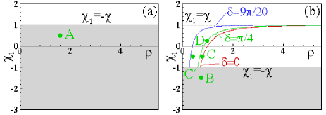
Figure 1: Domains of the MI: shaded regions in both panels, as well as the region under the respective curve, corresponding to different gain/loss coefficient ($\delta$), in panel (b), in the $(\chi_{1},\rho)$-plane for different $\delta$ (as indicated in the panels) and for fixed XPM coefficients, $\chi=-1$ (a), or $\chi=1$ (b). Capital letters indicate parameters chosen for displaying the evolution in figures following below.

Different origins of the MI should naturally lead to different scenarios of its development, which we studied by means of direct numerical simulations of Eqs. (1), (2). The simulations were performed subject to periodic boundary conditions, and with initial excitation of the CW state (6) by adding random noise with the amplitude amounting to 1$\%$ of that of the unperturbed background.

Starting with the case of weak gain and loss, defined by the symmetric solution ($\delta<\pi/2$), in Fig. 2 we show typical results of these simulations for the focusing XPM [see Fig. 2(a), with parameters corresponding to point A in Fig. 1(a)], and for the defocusing XPM [see Figs. 2(b)-(d), with parameters corresponding to points B-D in Fig. 1(b), respectively]. In panel (a) we observe a “standard” scenario of the development of MI. This behavior, being seemingly expectable, nevertheless reveals a noteworthy feature of the $\mathcal{PT}$-symmetric system, which behaves similarly to its Hamiltonian counterpart (at least, in significant initial intervals of the propagation). In particular, we observe that the power is distributed between the two waveguides.

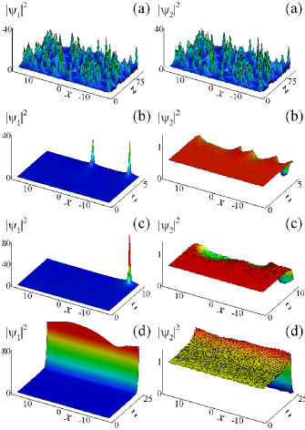
Figure 2: The evolution of field components $|\psi_{1}(x,z)|^{2}$ and $|\psi_{2}(x,z)|^{2}$ (left and right columns) of the plane-wave solution with parameters $k=0$, $\delta=\pi/4$, $\rho=1.604$, $\chi_{1}=0.5$, $\chi=-1$ (a), $\rho=0.76$, $\chi_{1}=-1.5$, $\chi=1$ (b), $\rho=0.79$, $\chi_{1}=-0.5$, $\chi=1$ (c) and $\rho=0.98$, $\chi_{1}=0.25$, $\chi=1$ (d). Parameters of panels (a), (b), (c) and (d) correspond to points A, B, C and D in Fig. 1, respectively.

The situation changes significantly when one consider the defocusing XPM, even if Eq. (9) is satisfied, i.e., the MI has the same nature as in the conservative system. Indeed, in Fig. 2(b) we observe a rather fast power transfer from the lossy waveguide to the one with the gain, accompanied by fast growing peaks. Obviously, such peaks can be described by a single NLS equation (1) with $\psi_{2}=0$. The observed behavior is due to the focusing SPM, $\chi_{1}$, and therefore is not significantly altered even when one passes from the domain of parameters (9) [Fig. 2(b)] to the one defined by Eq. (10), as shown in Fig. 2(c). A significant change, i.e., the third scenario of the evolution of the MI, appears when the SPM is defocusing too [Fig. 2(d)]. This is the case where the MI occurs only due to the imbalance of the gain and loss, resulting in nearly homogeneous grow (decay) of the field in the waveguide with gain (dissipation), respectively.

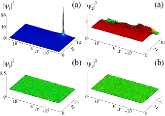
Figure 3: The evolution of field components $|\Psi_{1}(x,z)|^{2}$ $|\Psi_{2}(x,z)|^{2}$ (left and right columns) of the plane-wave solution with parameters $k=0.2$, $\delta=\pi/4$, $\chi_{1}=-0.5$, $\chi=1$, $\rho=0.79$ (a), or $\rho=0.4$ (b). Parameters of panels (a),(b) correspond to points C, C^′ in Fig. 1(b), respectively.

Examples of the modulational instability and stability for the CW solution with nonzero wave vector $k$ (current) are presented in Fig. 3. Here we restrict our consideration of the MI with the focusing SPM, $\chi_{1}<0$, but when $\chi_{1}+\chi<0$ [point C in Fig. 1(b)]. Thus, the evolution of the MI in this case occurs according to the same scenario as for $k=0$, cf. Figs .2(c) and Fig.3(a). At the same time, the respective MI peak is shifted in the positive direction of the $x$-axis, which coincides with the direction of the current. Meanwhile, in the domain where the CW state is predicted to be stable [above the green line, in Fig.1(b) — e.g., at point C^′ ], the stability is confirmed by the numerical simulations, see Fig.3(b).

4 The Peregrine soliton in $\mathcal{PT}$-symmetric system: the case of $\chi_{1}+\chi<0$

Turning now towards studying the Peregrine soliton (rogue wave) propagating against an unstable background we start with the case (9). This readily allows one to write down the Peregrine solution of Eqs. (1), (2) in the form ($j=1,2$) [40, 45]

$$\psi_{j}(x,z) = \rho e^{(-1)^{j}i\delta/2+ikx-ibz}\times$$ (13)

$$\left[1-4\frac{1-2i\left(\chi_{1}+\chi\right)\rho^{2}z}{1-2\left(\chi_{1}+\chi\right)\rho^{2}(x-2kz)^{2}+4\left(\chi_{1}+\chi\right)^{2}\rho^{4}z^{2}}\right].$$

Notice that, when $|z|\rightarrow\infty$, or, equivalently, $|x|\rightarrow\infty$, solution (13) merges into the background given by Eq. (6). Below, we separately consider two cases: the Peregrine soliton, based on the background without the current ($k=0$), and current-based Peregrine solution, with $k\neq 0$.

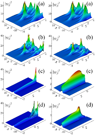
Figure 4: Peregrine solutions in the $\mathcal{PT}$-limit for $\rho=1.604$, $\chi_{1}=0.5$, $\chi=-1$, $\delta=\pi/4$ (a), or $\delta=3\pi/4$ (b); $\rho=0.76$, $\chi_{1}=-1.5$, $\chi=1$, $\delta=\pi/4$ (c), or $\delta=3\pi/4$ (d). Parameters of panels (a) and (b) correspond to the point A, while those of panels (c) and (d) – to point B in Fig.1.

Examples of the Peregrine solutions whose backgrounds (without the current, $k=0$) correspond to points A and B in Fig. 1, are depicted in Fig. 4. The spatial evolution of $|\psi_{j}(x,z)|^{2}$ was obtained by the numerical simulations of Eqs.(1), (2) with the initial condition corresponding to the Peregrine soliton (13) at $z=z_{i}=-4$ [Figs. 4(a) and 4(b)], or $z=z_{i}=-2$ [Figs. 4(c) and 4(d)]. In the case of the defocusing SPM and focusing XPM [Figs.4(a) and 4(b)], the central peak, corresponding to the Peregrine solution, appears at $x=z=0$, before MI peaks. At the same time, in the case of the focusing SPM and defocusing XPM [Figs. 4(c) and 4(d)], the appearance of the Peregrine-soliton peak at $x=z=0$ causes further growth of the peak in the first (gain-pumped) component, and decrease in the second (lossy) core. Notice that the structure of the rogue-wave evolution in this case resembles the respective scenario of the MI development for the same parameters, as suggested by the comparison of Figs. 2(b) and Figs. 4(c).

In the case when the background carries the current ($k\neq 0$), the central peak of the Peregrine solution moves with group velocity $2k$ in the positive direction of $x$-axis, as seen in Eq.(13) and confirmed by Figs. 5(a,b). Also for the focusing-XPM ($\chi<0$) case, the $\mathcal{PT}$-symmetric ($\delta<\pi/2$) rogue wave is more “stable” (in the sense that the MI peaks appear after at a longer propagation distance after the principal rogue-wave peak), see Fig.5(a), if compared to the $\mathcal{PT}$-antisymmetric wave with $\delta>\pi/2$, see Fig. 5(b).

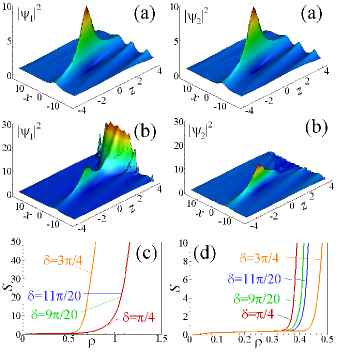
Figure 5: (a,b) Current-based Peregrine solutions in the $\mathcal{PT}$-symmetric system for $k=0.6$, $\rho=1.0$, $\chi_{1}=0.5$, $\chi=-1$, and $\delta=\pi/4$ (a), or $\delta=3\pi/4$ (b); (c,d) Discrepancy $S$ vs amplitude $\rho$ for different gain/loss coefficients $\delta$ (indicated in panels) and for $\chi_{1}=0.5$ and the focusing XPM, with $\chi=-1$ (c) or $\chi_{1}=-1.5$ and the defocusing XPM, with $\chi=1$.

In order to describe this rogue wave “stability” quantitatively, we will use one of the principal properties of Peregrine solution, which follows from Eq. (13), namely $\overline{\psi}_{j}(-x,-z)=\psi_{3-j}(x,z)$. If the phase of the solution is not taken into account, this property turns into $|\psi_{j}(-x,-z)|^{2}=|\psi_{j}(x,z)|^{2}$. Thus, we introduce the discrepancy as

$$S=\int_{-\infty}^{\infty}\!\left[\left|\psi_{1}(-x,-z_{i})\right|^{2}+\left|\psi_{2}(-x,-z_{i})\right|^{2}-\left|\psi_{1}(x,z_{i})\right|^{2}-\left|\psi_{2}(x,z_{i})\right|^{2}\right]^{2}dx,$$

in order to eliminate phase effects. In the ideal case, where the shape of the rogue wave coincides with the Peregrine solution (13), the discrepancy is zero, $S\equiv 0$. Thus, $S$ serves to measure how much the numerically obtained solution differs from the Peregrine soliton, or in other words, how much the chaotic nature of MI influences the Peregrine solution. The results are depicted in Figs. 5(c) and 5(d). For the focusing XPM [Fig.5(c)] and for $\delta\lesssim\pi/2$ the discrepancy abruptly grows at $\rho\gtrsim 1$. In the same time, in this range of $\delta$ the discrepancy almost does not depend on $\delta$ [the lines for $\delta=\pi/4$, $\delta=9\pi/20$, and $\delta=11\pi/20$ are indistinguishable on the scale of Fig. 5(c)]. Meanwhile, for $\delta>\pi/2$ the situation is opposite: the discrepancy increases with $\delta$ (compare the lines for $\delta=11\pi/20$ and $\delta=3\pi/4$). For the defocusing XPM [Fig. 5(d)], discrepancy $S$ decreases with the increase of $\delta$ in the whole range of $0\leq\delta\leq\pi$, while an abrupt growth happens at $\rho\gtrsim 0.4$. As a result, for the focusing XPM, the $\mathcal{PT}$-symmetric rogue wave with $\delta<\pi/2$ is more stable than the its antisymmetric counterpart, while for the defocusing XPM the situation is opposite.

5 Bright solitons

Obvious bright-soliton solutions of Eq. (5) with arbitrary amplitude $\eta$ are available too, for $\chi_{1}+\chi<0$:

$$\psi_{j}=\frac{\eta}{\sqrt{|\chi_{1}+\chi|}\cosh\left(\eta x/\sqrt{2}\right)}\exp\left[i\left((-1)^{j}\frac{\delta}{2}+\cos\delta+\frac{1}{2}\eta^{2}\right)z\right],$$ (14)

$j=1,2$, where, as above, intervals $0\leq\delta\leq\pi/2$ and $\pi/2\leq\delta\leq\pi$ correspond for the $\mathcal{PT}$-symmetric and antisymmetric solitons, respectively. Using results from Refs. [11] and [47], an exact stability boundary for the symmetric and antisymmetric solitons, against small perturbations breaking the respective symmetry or antisymmetry, can be predicted in the following analytical form:

$$\eta_{\mathrm{cr}}^{2}=\frac{16\left(-\chi_{1}-\chi\right)\cos\delta}{\left(\sqrt{-25\chi_{1}+7\chi}-3\sqrt{-\chi_{1}-\chi}\right)\left(\sqrt{-25\chi_{1}+7\chi}+\sqrt{-\chi_{1}-\chi}\right)},$$ (15)

the solitons being stable at $\eta^{2}<\eta_{\mathrm{cr}}^{2}$.

This result makes sense when Eq. (15) yields a positive value, otherwise the $\mathcal{PT}$-symmetry-breaking bifurcation does not occur, and the stability may only be studied numerically [in addition to the instability mode represented by Eq. (15), other instabilities are possible too]. In particular, condition (15) cannot simultaneously hold for the $\mathcal{PT}$-symmetric and antisymmetric solitons. Further, because the existence of the solitons of either type requires $\chi_{1}+\chi<0$, the condition of $\eta_{\mathrm{cr}}^{2}>0$ actually holds for the $\mathcal{PT}$-symmetric solitons at $-\chi_{1}>-\chi$, and for the $\mathcal{PT}$-antisymmetric solitons — in the opposite case, at $-\chi_{1}<-\chi$.

We have performed direct simulations of the evolution of perturbed solitons within the framework of Eqs. (1) and (2), aiming to identify stability borders for the $\mathcal{PT}$-symmetric and anti-symmetric solitons, and, in particular, to verify the analytical prediction (15). Perturbations were introduced by adding $2\%$ to the amplitude of component, and reducing $2\%$ from the other. Figures 6(a) and 6(b) display the so identified stability boundaries in the cases of opposite and identical signs of $\chi$ and $\chi_{1}$, respectively. For the sake of comparison with Ref. [11, 12], we demonstrate these borders as a function of $\gamma$ , rather than $\delta$ [see Eq. (3)].

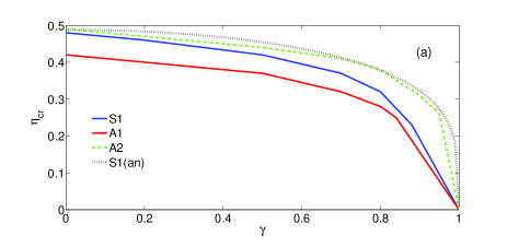
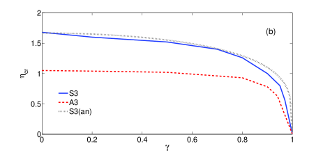
Figure 6: (a) Stability boundaries for $\mathcal{PT}$-symmetric and antisymmetric solitons (14) are shown in the plane of the gain-loss coefficient $\gamma$ (recall $\gamma\equiv\sin\delta$) and soliton’s amplitude $\eta$, in the case of opposite signs of the SPM and XPM coefficients. The boundaries for the $\mathcal{PT}$-symmetric (S1) and antisymmetric (A1) solitons are shown by solid blue and red lines, respectively, for $\chi=1$ and $\chi_{1}=-1.5$. The dotted black curve labeled S1(an) displays the analytical counterpart of the S1 boundary, as predicted by Eq. (15). The stability boundary for antisymmetric solitons, depicted by the dashed green curve (A2), pertains to $\chi=-1$ and $\chi_{1}=0.5$. (b) The stability boundaries in case of identical signs of the SPM and XPM coefficients, $\chi=-1$ and $\chi_{1}=-3$. The boundaries (S3) and (A3) for symmetric and antisymmetric solitons are shown by solid blue (S) and dashed red curves (A), respectively. The dotted black curve labeled S3(an) is the analytical counterpart of the latter boundary, as predicted by Eq. (15).

The numerically found stability boundaries are close to their analytical counterparts. Some discrepancy between them is explained by the fact that some solitons, which are stable against infinitesimal perturbations, may be destabilized by finite-amplitude excitations.

Typical examples of the unstable and stable evolution of antisymmetric solitons, taken on both sides of the stability boundary, are demonstrated in Fig.7, for $\chi=-1$ and $\chi_{1}=0.5$. The quick stabilization of the symmetric soliton in the same case is demonstrated in Fig.8 for a large amplitude, $\eta=3$. Actually, the $\mathcal{PT}$-symmetric solitons are stable for all $\eta$ in this case, the stability border being relevant for the antisymmetric ones.

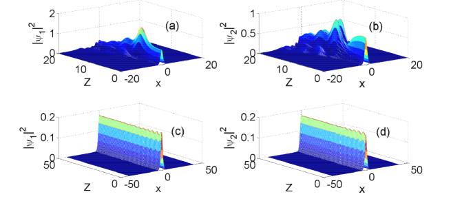
Figure 7: Stable and unstable evolution of both components of antisymmetric solitons (14) at $\chi=-1$ , $\chi_{1}=0.5$ and $\delta=\pi-\arcsin(0.2)$. Panels (a) and (b) pertain to the unstable dynamics of the soliton with amplitude $\eta=0.6$, while panels (c) and (d) pertain to the stable soliton with $\eta=0.3$.

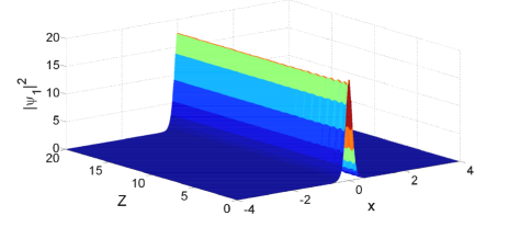
Figure 8: Quick stabilization of a symmetric soliton with a large value, $\eta=3$, for $\chi=-1$, $\chi_{1}=0.5$ and $\gamma=0.2$. Dynamics of the $v$-component is similar to that shown here for the $u$-component.

It is relevant to note too that, in the Manakov’s limit, $\chi_{1}=\chi$ [44], the stability boundary predicted by Eq. (15) diverges. Indeed, direct simulations demonstrate that all the solitons are stable in this case.

6 Conclusion

In this work we have considered the MI (modulational instability) of CW backgrounds and the emergence and evolution of rogue waves in the system of linearly-coupled $\mathcal{PT}$-symmetric coupled NLSEs. We have shown that the focusing XPM nonlinear interactions extend the effective stability region for the rogue waves of the Peregrine’s type. The system can support nondissipative rogue waves too. The stability region for $\mathcal{PT}$-symmetric and antisymmetric solitons was found in the exact analytical form and verified by direct simulations. It may be interesting to extend the analysis for (2D) versions of the system, which may have realizations in nonlinear optics, cf. Ref. [48] and references therein.

References

References

- [1] Akhmediev N and Pelinovsky E, 2010 Eur. Phys. J. Special Topics 185 1
- [2] Soto-Crespo, J M, Grelu P and Akhmediev N 2011 Phys. Rev. E 84 016604.
- [3] Bender C M and Boettcher S 1998, Phys. Rev. Lett.80 5243
- [4] Bender C N 2007 Rep. Prog. Phys. 70, 947
- [5] Rüter C E, Makris K G, El-Ganainy R, Christodoulides D N, Segev M, and Kip D, 2010 Nature Phys. 6 192
- [6] Benisty H, Degiron A, Lupu A, De Lustrac A, Chénais S, Forget S, Besbes M, . Barbillon G, Bruyant A, Blaize S and Léronde G 2011 Opt. Express 19 18004
- [7] Hang C, Huang G, and Konotop V. V. 2013, Phys. Rev. Lett.110, 083604.
- [8] Solli D R , Ropers C, Koonath P, and Jalali B, 2007, Nature 450 1054
- [9] Kibler B, Fatome J, Finot C, Millot G, Dias F, Genty G, Akhmediev N, and Dudley J M, 2010 Nature Phys. 6 790
- [10] Bludov Y V, Konotop V V and Akhmediev N 2009 Opt. Lett. 34 3015
- [11] Driben R and Malomed B A, 2011 Opt. Lett. 36 4323
- [12] Driben R and Malomed B A, 2011 EPL 94 3 37011
- [13] Alexeeva N V, Barashenkov I V, Sukhorukov A A, and Kivshar Y S, 2012 Phys. Rev.A 85 063837
- [14] Leykam D, Konotop V V, and Desyatnikov A S , 2013 Opt. Lett. 38 371
- [15] Barashenkov I V, Baker L, and Alexeeva N V , 2013 Phys. Rev.A 87 033819
- [16] Bludov Y V, Konotop V V, and Malomed B A, 2013 Phys. Rev.A 87, 013816
- [17] Barashenkov I V, Suchkov S V, Sukhorukov A A, Dmitriev S V, and Kivshar Y S 2012 Phys. Rev.A 86, 053809
- [18] Abdullaev F K, Konotop V V, Ögren M, and Sørensen M P, 2011 Opt. Lett. 36, 4566.
- [19] Ranka J K, Windeler R S, and Stentz A J, 2000 Opt. Lett. 25, 25.
- [20] Herrmann J, Griebner U, Zhavoronkov N, Husakou A, Nickel D, Knight J C, Wadsworth W J, Russell P St J, and Korn G 2002 Phys. Rev. Lett.88 173901
- [21] Dudley J M, Genty G, and Coen S, 2006 Rev. Mod. Phys. 78 1135
- [22] Skryabin D V and Gorbach A V, 2010 Rev. Mod. Phys. 82 1287
- [23] Driben R, Husakou A, Herrmann J, 2009 Opt. Lett. 34 2132
- [24] Satsuma J and Yajima N, 1974 Progr. Theor. Phys. Suppl. 55, 284
- [25] Driben R, Malomed B A, Skryabin D V, Yulin A V 2013, submitted to Opt. Lett.
- [26] Efimov A, Yulin A V, Skryabin D V, Knight J C, Joly N, Omenetto F G, Taylor A J, Russell P, 2005 Phys. Rev. Lett.95 213902
- [27] Driben R, Mitschke F, and Zhavoronkov N, 2010 Opt. Express 18 25993
- [28] Mitschke F M and Mollenauer L F, 1986 Opt. Lett. 11 659
- [29] Dudley J M, Genty G, and Eggleton B J, 2008 Opt. Express 16 3644
- [30] Genty G, de Sterke C M, Bang O, Dias F, Akhmediev N, Dudley J M 2010 Phys. Lett. A 374 989
- [31] Driben R and Babushkin I V 2012 Opt. Lett. 37 5157
- [32] Demircan A, Amiranashvili S, Bree C, Mahnke C, Mitschke F and Steinmeyer G 2012 Scientific Reports 2 850
- [33] Dudley J M, Genty G, Dias F, Kibler B, and Akhmediev N 2009 Opt. Exp. 17 21497
- [34] Akhmediev N, Soto-Crespo J M, and Ankiewicz A, 2009 Phys. Lett. A 373, 2137
- [35] Akhmediev N, Soto-Crespo J M, and Ankiewicz A, 2009 Phys. Rev.A 80, 043818
- [36] Akhmediev N and Korneev V I, 1986 Theor. Math. Phys. 69, 1089
- [37] Peregrine D H 1983 J. Austral. Math. Soc. B 25 16
- [38] Akhmediev N, Ankiewicz A, and Taki M, 2009 Phys. Lett. A 373, 675
- [39] Kharif C, Pelinovsky E, and Slunyaev A, Rogue Waves in the Ocean (Springer: 2009)
- [40] Bludov Yu V, Konotop V V, and Akhmediev N, 2010 Eur. Phys. J. Special Topics 185, 169
- [41] Baronio F, Degasperis A, Conforti M, Wabnitz S and Branze, V 2012 Phys. Rev. Lett.109 044102
- [42] Malomed B A and Winful 1996 Phys. Rev. E 53 5365; Atai J and Malomed B A 1996 Phys. Rev.E 54 4371
- [43] Dror N, Malomed B A, and Zeng J 2011, Phys. Rev. E 84, 046602
- [44] Manakov S V 1973, Zhurn. Eksp. Teor. Fiz. 65 505
- [45] Chabchoub A, Hoffmann N, and Akhmediev N, 2011 Phys. Rev. Lett.106, 204502
- [46] Soto-Crespo J M and Akhmediev N, 1993 Phys. Rev.E 48, 4710
- [47] Sakaguchi H and Malomed B A, 2011 Phys. Rev.E 83, 036608
- [48] Paulau P V, Gomila D, Colet P, Malomed B A, and Firth W J 2011 Phys. Rev.E 84 036213