Parabolic Harnack inequality of viscosity solutions on Riemannian manifolds

Abstract.

We consider viscosity solutions to nonlinear uniformly parabolic equations in nondivergence form on a Riemannian manifold $M$, with the sectional curvature bounded from below by $-\kappa$ for $\kappa\geq 0$. In the elliptic case, Wang and Zhang [WZ] recently extended the results of [Ca] to nonlinear elliptic equations in nondivergence form on such $M$, where they obtained the Harnack inequality for classical solutions. We establish the Harnack inequality for nonnegative viscosity solutions to nonlinear uniformly parabolic equations in nondivergence form on $M$. The Harnack inequality of nonnegative viscosity solutions to the elliptic equations is also proved.

1. Introduction and main results

In this paper, we study the Harnack inequality of viscosity solutions to nonlinear uniformly parabolic equations in nondivergence form on Riemannian manifolds. Let $(M,g)$ be a smooth, complete Riemannian manifold of dimension $n$. Consider a nonlinear uniformly parabolic equation

(1) $$F(D^{2}u)-\partial_{t}u=f\quad\mbox{in}\,\,\,M\times{\mathbb{R}},$$

where $D^{2}u$ denotes the Hessian of the function $u$ defined by

$$D^{2}u\,(X,Y)=g\left(\nabla_{X}\nabla u,Y\right),$$

for any vector fields $X,Y$ on $M,$ and $\nabla u$ is the gradient of $u.$ We notice that in the case, when $F$ is the trace operator, (1) is the well-known heat equation with a source term.

In the setting of elliptic equations on $M,$ Cabré [Ca] established the Krylov-Safonov type Harnack inequality of classical solutions to linear, uniformly elliptic equations in nondivergence form, when $M$ has nonnegative sectional curvature. The Krylov-Safonov Harnack inequality is based on the Aleksandrov-Bakelman-Pucci (ABP) estimate, which is proved using affine functions in the Euclidean case. Since affine functions can not be generalized into an intrinsic notion on Riemannian manifolds, Cabré considered the functions of the squared distance instead of the affine functions to overcome the difficulty. Later, Kim [K] improved Cabré’s result removing the sectional curvature assumption and imposing the certain condition on the distance function (see [K, p. 283]). Recently, Wang and Zhang [WZ] obtained a version of the ABP estimate on $M$ with Ricci curvature bounded from below, and the Harnack inequality of classical solutions for nonlinear uniformly elliptic operators provided that $M$ has a lower bound of the sectional curvature.

In the parabolic case, the Krylov-Safonov Harnack inequality was proved in [KKL] for classical solutions to linear, uniformly parabolic equations in nondivergence form, assuming essentially the same condition introduced by Kim [K]. The result in [KKL], in particular, gives a non-divergent proof of Li-Yau’s Harnack inequality for the heat equation in a manifold with nonnegative Ricci curvature [LY]. The ABP-Krylov-Tso estimate discovered by Krylov [Kr] in the Euclidean case (see also [T, W]) is a parabolic analogue of the ABP estimate, and a key ingredient in proving the parabolic Harnack inequality. In order to prove the ABP-Krylov-Tso type estimate on Riemannian manifolds , an intrinsically geometric version of the Krylov-Tso normal map, namely,

$$\Phi(x,t):=\left(\exp_{x}\nabla_{x}u(x,t),-\frac{1}{2}d^{2}\left(x,\exp_{x}\nabla u(x,t)\right)-u(x,t)\right)$$

was introduced. The map $\Phi$ is called the parabolic normal map related to $u(x,t)$ and the Jacobian determinant of $\Phi$ was explicitly computed in [KKL, Lemma 3.1].

In this paper, we shall prove the Krylov-Safonov Harnack inequality for a class of viscosity solutions to uniformly parabolic equations on $M$ with the sectional curvature bounded from below. Let $\operatorname{Sym}TM$ be the bundle of symmetric 2-tensors over $M.$ A nonlinear operator $F:\operatorname{Sym}TM\rightarrow{\mathbb{R}}$ will be always assumed in this article to satisfy the following basic hypothesis:

1. $F$ is uniformly elliptic with the so-called ellipticity constants $0<\lambda\leq\Lambda,$ i.e., for any $S\in\operatorname{Sym}TM,$ and for any positive semidefinite $P\in\operatorname{Sym}TM,$

   (H1) $$\lambda\,\mathrm{trace}(P_{x})\leq F(S_{x}+P_{x})-F(S_{x})\leq\Lambda\,\mathrm{trace}(P_{x}),\quad\forall x\in M.$$

We may assume that $0<\lambda\leq 1\leq\Lambda.$ In order to establish the uniform Harnack inequality for a class of uniformly parabolic equations including (1), we introduce Pucci’s extremal operators as in [CC]: for any $x\in M,$ and $S_{x}\in\operatorname{Sym}TM_{x},$

$${\mathcal{M}}^{+}_{\lambda,\Lambda}(S_{x}):={\mathcal{M}}^{+}(S_{x})=\lambda\sum_{e_{i}<0}e_{i}+\Lambda\sum_{e_{i}>0}e_{i},$$

$${\mathcal{M}}^{-}_{\lambda,\Lambda}(S_{x}):={\mathcal{M}}^{-}(S_{x})=\Lambda\sum_{e_{i}<0}e_{i}+\lambda\sum_{e_{i}>0}e_{i},$$

where $e_{i}=e_{i}(S_{x})$ are the eigenvalues of $S_{x}.$ In terms of the Pucci operators, the hypothesis (H1) of uniform ellipticity is equivalent to the following: for any $S,P\in\operatorname{Sym}TM,$

(H1’) $${\mathcal{M}}^{-}(P_{x})\leq F(S_{x}+P_{x})-F(S_{x})\leq{\mathcal{M}}^{+}(P_{x}),\quad\forall x\in M.$$

Now we recall viscosity solutions, which are proper weak solutions for nonlinear equations in nondivergence form. In the Euclidean space, the existence, uniqueness and regularity theory for the viscosity solutions have been developed by many authors (see for instance, [CIL, CC, W]). In [AFS, Z], the concept of viscosity solutions has been naturally extended on Riemannian manifolds, which can be found in Definitions 2.13 and 5.3. The authors in [AFS, PZ, Z] have shown comparison, uniqueness and existence results for the viscosity solutions on Riemannian manifolds. Using Pucci’s extremal operators, we introduce a class of viscosity solutions to the uniformly parabolic equations; see [CC].

Definition 1.1.

Let $\Omega\subset M$ be open, $T>0,$ and $0<\lambda\leq\Lambda.$ We denote by $\overline{\mathcal{S}}_{P}\left(\lambda,\Lambda,f\right)$ a class of a viscosity supersolution $u\in C(\Omega\times(0,T])$ satisfying

$${\mathcal{M}}^{-}(D^{2}u)-\partial_{t}u\leq f\quad\mbox{in $\Omega\times(0,T]$}$$

in the viscosity sense. Similarly, a class of viscosity subsolutions $\underline{{\mathcal{S}}}_{P}\left(\lambda,\Lambda,f\right)$ is defined as the set of $u\in C(\Omega\times(0,T])$ such that

$${\mathcal{M}}^{+}(D^{2}u)-\partial_{t}u\geq f\quad\mbox{in $\Omega\times(0,T]$}$$

in the viscosity sense. We denote

$${\mathcal{S}}_{P}^{*}\left(\lambda,\Lambda,f\right):=\overline{\mathcal{S}}_{P}\left(\lambda,\Lambda,|f|\right)\cap\underline{{\mathcal{S}}}_{P}\left(\lambda,\Lambda,-|f|\right).$$

Simply, we write $\overline{\mathcal{S}}_{P}(f),$ $\underline{{\mathcal{S}}}_{P}(f),$ and ${\mathcal{S}}_{P}^{*}(f)$ for $\overline{\mathcal{S}}_{P}\left(\lambda,\Lambda,f\right),$ $\underline{{\mathcal{S}}}_{P}\left(\lambda,\Lambda,f\right),$ and ${\mathcal{S}}_{P}^{*}\left(\lambda,\Lambda,f\right),$ respectively.

Note that the viscosity solution to the fully nonlinear uniformly parabolic equation (1) belongs to the class ${\mathcal{S}}_{P}^{*}\left(\lambda,\Lambda,f-F(0,\cdot)\right)$ owing to the equivalence between (H1) and (H1’).

To obtain the Harnack inequality of viscosity solutions contained in ${\mathcal{S}}_{P}^{*}$ from a priori Harnack estimates (Subsection 4.1, [KKL], and [Ca, K, WZ]), we use regularization by sup and inf-convolutions, introduced by Jensen [J]. The classical ABP estimate for viscosity solutions was proved by making use of affine functions, especially the convex envelope of the viscosity solution (see [CC, W]). Replacing affine functions by the squared distance functions on $M,$ as mentioned above, we consider the sup and inf-convolutions on Riemanninan manifolds defined as follows: for $\varepsilon>0,$ let $u_{\varepsilon}$ denote the inf-convolution of $u$, defined as

$$u_{\varepsilon}(x):=\inf_{y\in\Omega}\left\{u(y)+\frac{1}{2\varepsilon}d^{2}(y,x)\right\},\qquad\forall x\in\Omega\subset M.$$

The sup-convolution can be defined in a similar way using concave paraboloids. We see that the regularized functions by the sup and inf-convolutions are semi-convex and semi-concave, respectively, which imply that they admit the Hessian almost everywhere thanks to the Aleksandrov theorem [A, B]. In Lemma 3.6, we prove that regularized viscosity solutions solve approximated equations in the viscosity sense, provided that the sectional curvature of $M$ is bounded from below, and the operator $F$ is intrinsically uniformly continuous with respect to $x$; see Definition 3.4. Intrinsic uniform continuity of Pucci’s operators is a sufficient condition for obtaining the uniform Harnack estimates for viscosity solutions since a class ${\mathcal{S}}^{*}_{P}$ of all viscosity solutions to the uniformly parabolic equations is invariant under the regularization processes of sup and inf-convolutions. Then an application of a priori estimates to the sup and inf-convolutions of viscosity solutions will yield the uniform Harnack inequality for viscosity solutions.

On the other hand, assuming the sectional curvature of $M$ to be bounded from below, we establish a priori Harnack inequality for nonlinear parabolic operators in Section 4.1 influenced by Wang and Zhang [WZ], who studied the elliptic case. We introduce the parabolic contact set ${\mathcal{A}}_{a,b}$ for $a,b>0$ in Definition 4.3, which consists of a point $(\overline{x},\overline{t})\in M\times{\mathbb{R}},$ where a concave paraboloid

$$-\frac{a}{2}d_{y}^{2}(x)+bt+C\,\,\,\mbox{(for some $C$)}$$

touches $u$ from below at $(\overline{x},\overline{t})$ in a parabolic neighborhood of $(\overline{x},\overline{t}),$ i.e, $B_{r}(\overline{x})\times(\overline{t}-r^{2},\overline{t}]$ for some $r>0.$ Under the assumption that Ricci curvature of $M$ is bounded from below, an estimation of the Jacobian of the parabolic normal map on the parabolic contact set ${\mathcal{A}}_{a,b}$ is obtained in Lemma 4.4, which is essential for proving the ABP-Krylov-Tso type estimate. For the heat equation on manifolds with a lower bound of the Ricci curvature, we can use Lemma 4.4 and Bishop-Gromov’s volume comparison theorem to deduce the Harnack inequality with help of the Laplacian comparison theorem. In particular, this implies a global Harnack inequality for heat equation on manifolds with nonnegative Ricci curvature proved earlier by Li and Yau [LY]; see Remarks 4.5 and 4.10. Regarding a class of nonlinear operators, we establish the (locally) uniform Harnack inequality for uniformly parabolic operators provided that the sectional curvature of the underlying manifold is bounded from below, where our computation does not rely on the linearity of the operator as in [WZ].

Now we state our main results as follows. In the statements and hereafter, we denote

$$\fint_{Q}f:=\frac{1}{|Q|}\int_{Q}f$$

and

$$K_{r}(x_{0},t_{0}):=B_{r}(x_{0})\times(t_{0}-r^{2},t_{0}],\quad(x_{0},t_{0})\in M\times{\mathbb{R}},$$

where $|Q|$ stands for the volume of a set $Q$ of $M$ or $M\times{\mathbb{R}},$ and $B_{r}(x_{0})$ is a geodesic ball of radius $r$ centered at $x_{0}.$

Theorem 1.2 (Parabolic Harnack inequality).

Assume that $M$ has sectional curvature bounded from below by $-\kappa$ for $\kappa\geq 0,$ i.e., $\operatorname{Sec}\geq-\kappa$ on $M.$ Let $0<R\leq R_{0},$ and $f\in C\left(K_{2R}(x_{0},4R^{2})\right).$ If $u\in C\left(K_{2R}(x_{0},4R^{2})\right)$ is a nonnegative viscosity solution in ${\mathcal{S}}_{P}^{*}\left(\lambda,\Lambda,f\right)$ in $K_{2R}(x_{0},4R^{2}),$ then we have

(2) $$\sup_{K_{R}(x_{0},2R^{2})}u\leq C_{H}\left\{\inf_{K_{R}(x_{0},4R^{2})}u+R^{2}\left(\fint_{K_{2R}(x_{0},4R^{2})}|{f}|^{n\theta+1}\right)^{\frac{1}{n\theta+1}}\right\},$$

where $\theta:=1+\log_{2}\cosh(8\sqrt{\kappa}R_{0})$ and $C_{H}>0$ is a uniform constant depending only on $n,\lambda,\Lambda$ and $\sqrt{\kappa}R_{0}$.

When $\kappa=0,$ (2) becomes a global Harnack inequality which extends the classical Euclidean theory of Krylov and Safonov [KS]. Assuming the sectional curvature to be bounded from below, our Harnack estimate are locally uniform, namely, for a fixed $R_{0}>0,$ we obtain uniform Harnack inequalities in any balls of radius $R$ less than $R_{0}.$ When $n,\lambda$ and $\Lambda$ are given, the uniform constant $C_{H}=C_{H}\left(\sqrt{\kappa}R_{0}\right)$ in our estimate (2) grows faster than $\exp\left(1+{\kappa}R_{0}^{2}\right)$ as $\sqrt{\kappa}R_{0}$ tends to infinity; see Remark 4.10.

Theorem 1.3 (Weak Harnack inequality).

Assume that $\operatorname{Sec}\geq-\kappa\,$ on $M$ for $\kappa\geq 0.$ Let $0<R\leq R_{0},$ and $f\in C\left(K_{2R}(x_{0},4R^{2})\right).$ If $u\in C\left(K_{2R}(x_{0},4R^{2})\right)$ is a nonnegative viscosity supersolution in $\overline{\mathcal{S}}_{P}\left(\lambda,\Lambda,f\right)$ in $K_{2R}(x_{0},4R^{2}),$ then we have

(3) $$\left(\fint_{K_{R}(x_{0},2R^{2})}u^{p}\right)^{\frac{1}{p}}\leq C_{H}\left\{\inf_{K_{R}(x_{0},4R^{2})}u+R^{2}\left(\fint_{K_{2R}(x_{0},4R^{2})}|{f^{+}}|^{n\theta+1}\right)^{\frac{1}{n\theta+1}}\right\};\quad f^{+}:=\max(f,0),$$

where $\theta:=1+\log_{2}\cosh(8\sqrt{\kappa}R_{0}),$ and the positive constants $p\in(0,1)$ and $C_{H}$ are uniform depending only on $n,\lambda,\Lambda,$ and $\sqrt{\kappa}R_{0}.$

In the elliptic setting, we have Harnack inequalities for a class of viscosity solutions as below; refer to Definition 5.3 for the definitions of classes ${\mathcal{S}}^{*}_{E}$ and $\overline{\mathcal{S}}_{E}$ of viscosity solutions and supersolutions to uniformly elliptic equations.

Theorem 1.4 (Elliptic Harnack inequality).

Assume that $\operatorname{Sec}\geq-\kappa\,$ on $M$ for $\kappa\geq 0.$ Let $0<R\leq R_{0},$ and $f\in C\left(B_{2R}(x_{0})\right).$ If $u\in C\left(B_{2R}(x_{0})\right)$ is a nonnegative viscosity solution in ${\mathcal{S}}_{E}^{*}\left(\lambda,\Lambda,f\right)$ in $B_{2R}(x_{0}),$ then we have

$$\sup_{B_{R}(x_{0})}u\leq C\left\{\inf_{B_{R}(x_{0})}u+R^{2}\left(\fint_{B_{2R}(x_{0})}|f|^{n\theta}\right)^{\frac{1}{n\theta}}\right\},$$

where $\theta:=1+\log_{2}\cosh\left(8\sqrt{\kappa}R_{0}\right)$ and $C>0$ is a uniform constant depending only on $n,\lambda,\Lambda,$ and $\sqrt{\kappa}R_{0}.$

Theorem 1.5 (Weak Harnack inequality).

Assume that $\operatorname{Sec}\geq-\kappa\,$ on $M$ for $\kappa\geq 0.$ Let $0<R\leq R_{0},$ and $f\in C\left(B_{2R}(x_{0})\right).$ If $u\in C\left(B_{2R}(x_{0})\right)$ is a nonnegative viscosity supersolution in $\overline{\mathcal{S}}_{E}\left(\lambda,\Lambda,f\right)$ in $B_{2R}(x_{0}),$ then we have

$$\left(\fint_{B_{R}(x_{0})}u^{p}\right)^{\frac{1}{p}}\leq C\left\{\inf_{B_{R}(x_{0})}u+R^{2}\left(\fint_{B_{2R}(x_{0})}|{f^{+}}|^{n\theta}\right)^{\frac{1}{n\theta}}\right\};\quad f^{+}:=\max(f,0),$$

where $\theta:=1+\log_{2}\cosh(8\sqrt{\kappa}R_{0})$ and the positive constants $p\in(0,1)$ and $C$ are uniform depending only on $n,\lambda,\Lambda,$ and $\sqrt{\kappa}R_{0}.$

The rest of the paper is organized as follows. In Section 2, we recall some results on Riemannian geometry and viscosity solutions that are used in the paper. In Section 3, we investigate basic properties of the sup and inf-convolutions, and the relation between the viscosity solution and its sup and inf-convolutions. Section 4 is devoted to proving the parabolic Harnack inequalities of viscosity solutions. In Section 5, we prove Harnack inequalities of viscosity solutions to the elliptic equations.

2. Preliminaries

2.1. Riemannian geometry

Let $(M,g)$ be a smooth, complete Riemannian manifold of dimension $n$, where $g$ is the Riemannian metric and $\operatorname{Vol}:=\operatorname{Vol}_{g}$ is the Riemannian measure on $M$. We denote $\langle X,Y\rangle:=g(X,Y)$ and $|X|^{2}:=\langle X,X\rangle$ for $X,Y\in T_{x}M$, where $T_{x}M$ is the tangent space at $x\in M$. Let $d(\cdot,\cdot)$ be the distance function on $M$. For a given point $y\in M$, $d_{y}(x)$ denotes the distance function to $y$, i.e., $d_{y}(x):=d(x,y)$.

We recall the exponential map $\exp:TM\to M$. If $\gamma_{x,X}:{\mathbb{R}}\to M$ is the geodesic starting at $x\in M$ with velocity $X\in T_{x}M$, then the exponential map is defined by

$$\exp_{x}(X):=\gamma_{x,X}(1).$$

We observe that the geodesic $\gamma_{x,X}$ is defined for all time since $M$ is complete. For $X\in T_{x}M$ with $|X|=1$, we define the cut time $t_{c}(X)$ as

$$t_{c}(X):=\sup\left\{t>0:\exp_{x}(sX)\,\,\,\mbox{is minimizing between}\,\,\,x\,\,\,\mbox{and $\exp_{x}(tX)$}\right\}.$$

The cut locus of $x\in M,$ denoted by $\operatorname{Cut}(x),$ is defined by

$$\operatorname{Cut}(x):=\left\{\exp_{x}(t_{c}(X)X):X\in T_{x}M\,\,\,\mbox{with $|X|=1,\,\,t_{c}(X)<+\infty$}\right\}.$$

If we define

$$E_{x}:=\left\{tX\in T_{x}M:0\leq t<t_{c}(X),\,\,X\in T_{x}M\,\,\,\mbox{with $|X|=1$}\right\}\subset T_{x}M,$$

it can be proved that $\operatorname{Cut}(x)=\exp_{x}(\partial E_{x}),M=\exp_{x}(E_{x})\cup\operatorname{Cut}(x),$ and $\exp_{x}:E_{x}\to\exp_{x}(E_{x})$ is a diffeomorphism. We note that $\operatorname{Cut}(x)$ is closed and has measure zero. Given two points $x$ and $y\notin\operatorname{Cut}(x)$, there exists a unique minimizing geodesic $\exp_{x}(tX)$ (for $X\in E_{x}$) joining $x$ to $y$ with $y=\exp_{x}(X),$ and we will write $X=\exp_{x}^{-1}(y)$. For any $x\notin\operatorname{Cut}(y)\cup\{y\}$, the distance function $d_{y}$ is smooth at $x,$ and the Gauss lemma implies that

$$\nabla d_{y}(x)=-\frac{\exp_{x}^{-1}(y)}{|\exp_{x}^{-1}(y)|},$$

and

$$\nabla(d^{2}_{y}/2)(x)=-\exp_{x}^{-1}(y).$$

The injectivity radius at $x$ of $M$ is defined as

$$i_{M}(x):=\sup\{r>0:\,\,\mbox{$\exp_{x}$ is a diffeomorphism from $B_{r}(0)$ onto $B_{r}(x)$}\}.$$

We note that $i_{M}(x)>0$ for any $x\in M$ and the map $x\mapsto i_{M}(x)$ is continuous.

We recall the Hessian of a $C^{2}$- function $u$ on $M$ defined as

$$D^{2}u\,(X,Y):=\left\langle\nabla_{X}\nabla u,Y\right\rangle,$$

for any vector fields $X,Y$ on $M,$ where $\nabla$ denotes the Riemannian connection of $M,$ and $\nabla u$ is the gradient of $u.$ The Hessian $D^{2}u$ is a symmetric 2-tensor in $\operatorname{Sym}TM,$ whose value at $x\in M$ depends only on $u$ and the values $X,Y$ at $x.$ By a canonical identification of the space of symmetric bilinear forms on $T_{x}M$ with the space of symmetric endomorphisms of $T_{x}M,$ the Hessian of $u$ at $x\in M$ can be also viewed as a symmetric endomorphism of $T_{x}M$:

$$D^{2}u(x)\cdot X=\nabla_{X}\nabla u,\quad\forall X\in T_{x}M.$$

We will write $D^{2}u(x)\,(X,X)=\left\langle D^{2}u(x)\cdot X,\,X\right\rangle$ for $X\in T_{x}M.$

Let $\xi$ be a vector field along a differentiable curve $\gamma:[0,a]\to M.$ We denote by $\frac{D\xi}{dt}(t)=\nabla_{\dot{\gamma}(t)}\xi(t),$ the covariant derivative of $\xi$ along $\gamma.$ A vector field $\xi$ along $\gamma$ is said to be parallel along $\gamma$ when

$$\frac{D\xi}{dt}(t)\equiv 0\quad\mbox{on}\,\,\,[0,a].$$

If $\gamma:[0,1]\to M$ is a unique minimizing geodesic joining $x$ to $y,$ then for any $\zeta\in T_{x}M,$ there exists a unique parallel vector field, denoted by $L_{x,y}\zeta(t),$ along $\gamma$ such that $L_{x,y}\zeta(0)=\zeta.$ The parallel transport of $\zeta$ from $x$ to $y$ , denoted by $L_{x,y}\zeta,$ is defined as

$$L_{x,y}\zeta:=L_{x,y}\zeta(1)\in T_{y}M,$$

which will induce a linear isometry $L_{x,y}:T_{x}M\to T_{y}M.$ We note that $L_{y,x}=L_{x,y}^{-1}$ and

(4) $$\left\langle L_{x,y}\zeta,\nu\right\rangle_{y}=\left\langle\zeta,L_{y,x}\nu\right\rangle_{x},\quad\forall\zeta\in T_{x}M,\,\,\,\nu\in T_{y}M.$$

We also define the parallel transport of a symmetric bilinear form along the unique minimizing geodesic; see [AFS, p. 311].

Definition 2.1.

Let $x,y\in M,$ and let $\gamma:[0,1]\to M$ be a unique minimizing geodesic joining $x$ to $y.$ For $S_{x}\in\operatorname{Sym}TM_{x},$ the parallel transport of $S_{x}$ from $x$ to $y,$ denoted by $L_{x,y}\circ S_{x},$ is a symmetric bilinear form on $T_{y}M$ satisfying

$$\left\langle\left(L_{x,y}\circ S_{x}\right)\cdot\nu,\nu\right\rangle_{y}:=\left\langle S_{x}\cdot\left(L_{y,x}\nu\right),L_{y,x}\nu\right\rangle_{x},\qquad\forall\nu\in T_{y}M.$$

Identifying the space of symmetric bilinear forms on $T_{y}M$ with the space of symmetric endomorphisms of $T_{y}M,$ $L_{x,y}\circ S_{x}$ can be considered as a symmetric endomorphism of $T_{y}M$ such that

$$\left(L_{x,y}\circ S_{x}\right)\cdot\nu=L_{x,y}\left(S_{x}\cdot\left(L_{y,x}\nu\right)\right),\qquad\forall\nu\in T_{y}M.$$

Then it is not difficult to check that $S_{x}$ and $L_{x,y}\circ S_{x}$ have the same eigenvalues.

Let the Riemannain curvature tensor be defined by

$$R(X,Y)Z=\nabla_{X}\nabla_{Y}Z-\nabla_{Y}\nabla_{X}Z-\nabla_{[X,Y]}Z.$$

For two linearly independent vectors $X,Y\in T_{x}M,$ we define the sectional curvature of the plane determined by $X$ and $Y$ as

$$\operatorname{Sec}(X,Y):=\frac{\langle R(X,Y)X,Y\rangle}{|X|^{2}|Y|^{2}-\langle X,Y\rangle^{2}}.$$

Let $\operatorname{Ric}$ denote the Ricci curvature tensor defined as follows: for a unit vector $X\in T_{x}M$ and an orthonormal basis $\{X,e_{2},\cdots,e_{n}\}$ of $T_{x}M,$

$$\operatorname{Ric}(X,X)=\sum_{j=2}^{n}\operatorname{Sec}(X,e_{j}).$$

As usual, $\operatorname{Ric}\geq\kappa$ on $M\,\,\,(\kappa\in{\mathbb{R}})$ stands for $\operatorname{Ric}_{x}\geq\kappa g_{x}$ for all $x\in M.$

We recall the first and second variations of the energy function (see for instance, [D]).

Lemma 2.2 (First and second variations of energy).

Let $\gamma:[0,1]\to M$ be a minimizing geodesic, and $\xi$ be a vector field along $\gamma.$ For small $\epsilon>0,$ let $h:(-\epsilon,\epsilon)\times[0,1]\to M$ be a variation of $\gamma$ defined as

$$h(r,t):=\exp_{\gamma(t)}r\xi(t).$$

Define the energy function of the variation

$$E(r):=\int_{0}^{1}\left|\frac{\partial h}{\partial t}(r,t)\right|^{2}dt,\qquad\mbox{for}\,\,\,r\in(-\epsilon,\epsilon).$$

Then, we have

1. $$E(0)=d^{2}\left(\gamma(0),\gamma(1)\right),$$

2. $$\frac{1}{2}E^{\prime}(0) =\left\langle\xi(1),\dot{\gamma}(1)\right\rangle-\left\langle\xi(0),\dot{\gamma}(0)\right\rangle,$$

3. $$\frac{1}{2}E^{\prime\prime}(0) =\int_{0}^{1}\left\{\left\langle\frac{D\xi}{dt},\frac{D\xi}{dt}\right\rangle-\left\langle R\left(\dot{\gamma}(t),\xi(t)\right)\dot{\gamma}(t),\,\xi(t)\right\rangle\right\}dt.$$

In particular, if a vector field $\xi$ is parallel along $\gamma,$ then we have $\frac{D\xi}{dt}\equiv 0$ and $\langle\xi,\dot{\gamma}\rangle\equiv C$ (for $C\in{\mathbb{R}}$ ) on $[0,1].$ In this case, we have the following estimate:

(5) $$E(r)=E(0)-r^{2}\int_{0}^{1}\left\langle R\left(\dot{\gamma}(t),\xi(t)\right)\dot{\gamma}(t),\,\xi(t)\right\rangle dt+o\left(r^{2}\right).$$

Now, we state some known results on Riemannian manifolds with a lower bound of the curvature. First, we have the following volume doubling property assuming Ricci curvature to be bounded from below (see [V] for instance).

Theorem 2.3 (Bishop-Gromov).

Assume that $\operatorname{Ric}\geq-(n-1)\kappa$ on $M$ for $\kappa\geq 0.$ For any $0<r<R,$ we have

(6) $$\frac{\operatorname{Vol}(B_{2r}(z))}{\operatorname{Vol}(B_{r}(z))}\leq 2^{n}\cosh^{n-1}\left(2\sqrt{\kappa}R\right).$$

We observe that the doubling property (6) implies that for any $0<r<R<R_{0},$

$$\frac{\operatorname{Vol}(B_{R}(z))}{\operatorname{Vol}(B_{r}(z))}\leq{\mathcal{D}}\,\left(\frac{R}{r}\right)^{\log_{2}{\mathcal{D}}},$$

where ${\mathcal{D}}:=2^{n}\cosh^{n-1}\left(2\sqrt{\kappa}R_{0}\right)$ is the so-called doubling constant. Using the volume doubling property, it is easy to prove the following lemma.

Lemma 2.4.

Assume that for any $z\in M$ and $0<r<2R_{0},$ there exists a doubling constant ${\mathcal{D}}>0$ such that

$$\operatorname{Vol}(B_{2r}(z))\leq{\mathcal{D}}\operatorname{Vol}(B_{r}(z)).$$

Then we have that for any $B_{r}(y)\subset B_{R}(z)$ with $0<r<R<R_{0},$

(7) $$\left\{\fint_{B_{r}(y)}\left|r^{2}f\right|^{n\theta}\right\}^{\frac{1}{n\theta}}\leq 2\left\{\fint_{B_{R}(z)}\left|R^{2}f\right|^{n\theta}\right\}^{\frac{1}{n\theta}};\qquad\theta:=\frac{1}{n}\log_{2}{\mathcal{D}}.$$

In particular, if the sectional curvature of $M$ is bounded from below by $-\kappa$ ($\kappa\geq 0$), then (7) holds with $\theta:=1+\log_{2}\cosh(4\sqrt{\kappa}R_{0}).$

In the parabolic setting, it follows from Lemma 2.4 that for any $0<r<R<R_{0},$

(8) $$\left\{\fint_{K_{r,\,\alpha r^{2}}(y,s)}\left|r^{2}f\right|^{n\theta+1}\right\}^{\frac{1}{n\theta+1}}\leq 2\alpha^{-\frac{1}{n\theta+1}}\left\{\fint_{K_{R}(z,t)}\left|R^{2}f\right|^{n\theta+1}\right\}^{\frac{1}{n\theta+1}},$$

where $K_{r,\alpha r^{2}}(y,s):=B_{r}(y)\times(s-\alpha r^{2},s]\subset K_{R}(z,t)=B_{R}(z)\times(t-R^{2},t]$ for $\alpha>0.$

We recall semi-concavity of functions on Riemannian manifolds which is a natural generalization of concavity. The work of Bangert [B] concerning semi-concave functions enables us to deal with functions that are not twice differentiable in the usual sense.

Definition 2.5.

Let $\Omega$ be an open set of $M.$ A function $\phi:\Omega\to{\mathbb{R}}$ is said to be semi-concave at $x_{0}\in\Omega$ if there exist a geodesically convex ball $B_{r}(x_{0})$ with $0<r<i_{M}(x_{0}),$ and a smooth function $\Psi:B_{r}(x_{0})\to{\mathbb{R}}$ such that $\phi+\Psi$ is geodesically concave on $B_{r}(x_{0}).$ A function $\phi$ is semi-concave on $\Omega$ if it is semi-concave at each point in $\Omega.$

The following local characterization of semi-concavity is quoted from [CMS, Lemma 3.11].

Lemma 2.6.

Let $\phi:\Omega\to{\mathbb{R}}$ be a continuous function and let $x_{0}\in\Omega,$ where $\Omega\subset M$ is open. Assume that there exist a neighborhood $U$ of $x_{0},$ and a constant $C>0$ such that for any $x\in U$ and $X\in T_{x}M$ with $|X|=1,$

$$\limsup_{r\to 0}\frac{\phi\left(\exp_{x}rX\right)+\phi\left(\exp_{x}-rX\right)-2\phi(x)}{r^{2}}\leq C.$$

Then $\phi$ is semi-concave at $x_{0}.$

Hessian bound for the squared distance function is the following lemma which is proved in [CMS, Lemma 3.12] using the formula for the second variation of energy. According to the local characterization of semi-concavity combined with Lemma 2.7, $d_{y}^{2}$ is semi-concave on a bounded open set $\Omega\subset M$ for any $y\in M,$ provided that the sectional curvature of $M$ is bounded from below.

Lemma 2.7.

Let $x,y\in M.$ If $\operatorname{Sec}\geq-\kappa\,\,(\kappa\geq 0)$ along a minimizing geodesic joining $x$ to $y,$ then for any $X\in T_{x}M$ with $|X|=1,$

$$\limsup_{r\to 0}\frac{d_{y}^{2}\left(\exp_{x}rX\right)+d_{y}^{2}\left(\exp_{x}-rX\right)-2d^{2}_{y}(x)}{r^{2}}\leq 2\sqrt{\kappa}d_{y}(x)\coth\left(\sqrt{\kappa}d_{y}(x)\right).$$

The following result from Bangert is an extension of Aleksandrov’s second differentiability theorem that a convex function has second derivatives almost everywhere in the Euclidean space [A] (see also [V, Chapter 14]) .

Theorem 2.8 (Aleksandrov-Bangert, [B]).

Let $\Omega\subset M$ be an open set and let $\phi:\Omega\to{\mathbb{R}}$ be semi-concave. Then for almost every $x\in\Omega,$ $\phi$ is differentiable at $x,$ and there exists a symmetric operator $A(x):T_{x}M\to T_{x}M$ characterized by any one of the two equivalent properties:

1. for $\xi\in T_{x}M,\,\,\,$ $A(x)\cdot\xi=\nabla_{\xi}\nabla\phi(x),$
   

2. $\phi(\exp_{x}\xi)=\phi(x)+\left\langle\nabla\phi(x),\xi\right\rangle+\frac{1}{2}\left\langle A(x)\cdot\xi,\xi\right\rangle+o\left(|\xi|^{2}\right)\quad\mbox{ as $\xi\to 0.$}$

The operator $A(x)$ and its associated symmetric bilinear from on $T_{x}M$ are denoted by $D^{2}\phi(x)$ and called the Hessian of $\phi$ at $x$ when no confusion is possible.

Let $M$ and $N$ be Riemannian manifolds of dimension $n$ and $\phi:M\to N$ be smooth. The Jacobian of $\phi$ is the absolute value of determinant of the differential $d\phi$, i.e.,

$$\operatorname{Jac}\phi(x):=|\det d\phi(x)|\quad\mbox{for $x\in M$}.$$

The following is the area formula, which follows easily from the area formula in Euclidean space and a partition of unity.

Lemma 2.9 (Area formula).

For any smooth function $\phi:M\times{\mathbb{R}}\to M\times{\mathbb{R}}$ and any measurable set $E\subset M\times{\mathbb{R}}$, we have

$$\int_{E}\operatorname{Jac}\phi(x,t)dV(x,t)=\int_{M\times{\mathbb{R}}}{\mathcal{H}}^{0}[E\cap\phi^{-1}(y,s)]dV(y,s),$$

where ${\mathcal{H}}^{0}$ is the counting measure.

2.2. Viscosity solutions

In this subsection, we consider a refined definition of viscosity solutions to parabolic equations slightly different from the usual definition in [Z]; see [W] for the Euclidean case.

Definition 2.10.

Let $\Omega\subset M$ be open and $T>0.$ Let $u:\Omega\times(0,T]\to{\mathbb{R}}$ be a lower semi-continuous function. We say that $u$ has a local minimum at $(x_{0},t_{0})\in\Omega\times(0,T]$ in the parabolic sense if there exists $r>0$ such that

$$u(x,t)\geq u(x_{0},t_{0})\quad\mbox{for all $(x,t)\in K_{r}(x_{0},t_{0}):=B_{r}(x_{0})\times(t_{0}-r^{2},t_{0}].$}$$

Similarly, we can define a local maximum in the parabolic sense.

Definition 2.11 (Viscosity sub and super- differentials).

Let $\Omega\subset M$ be open and $T>0.$ Let $u:\Omega\times(0,T]\to{\mathbb{R}}$ be a lower semi-continuous function. We define the second order parabolic subjet of $u$ at $(x,t)\in\Omega\times(0,T]$ by

$${\mathcal{P}}^{2,-}u(x,t):= \left\{\left(\partial_{t}\varphi(x,t),\nabla\varphi(x,t),D^{2}\varphi(x,t)\right)\in{\mathbb{R}}\times T_{x}M\times\operatorname{Sym}TM_{x}:\varphi\in C^{2,1}\left(\Omega\times(0,T]\right),\right.$$

$$\left.\,\,u-\varphi\,\,\,\mbox{has a local minimum at $(x,t)$ in the parabolic sense}\right\}.$$

If $(p,\zeta,A)\in{\mathcal{P}}^{2,-}u(x,t),$ then $(p,\zeta)$ and $A$ are called a first order subdifferential (with respect to $(t,x)$), and a second order subdifferential (with respect to $x$) of $u$ at $(x,t),$ respectively.

In a similar way, for an upper semi-continuous function $u:\Omega\times(0,T]\to{\mathbb{R}},$ we define the second order parabolic superjet of $u$ at $(x,t)\in\Omega\times(0,T]$ by

$${\mathcal{P}}^{2,+}u(x,t):= \left\{\left(\partial_{t}\varphi(x,t),\nabla\varphi(x,t),D^{2}\varphi(x,t)\right)\in{\mathbb{R}}\times T_{x}M\times\operatorname{Sym}TM_{x}:\varphi\in C^{2,1}\left(\Omega\times(0,T]\right),\right.$$

$$\left.\,\,u-\varphi\,\,\,\mbox{has a local maximum at $(x,t)$ in the parabolic sense}\right\}.$$

The following characterization of the parabolic subjet ${\mathcal{P}}^{2,-}u$ can be obtained by a simple modification of [AFS, Proposition 2.2], [Z, Proposition 2.2].

Lemma 2.12.

Let $u:\Omega\times(0,T]\to{\mathbb{R}}$ be a lower semi-continuous function and let $(x,t)\in\Omega\times(0,T].$ The following statements are equivalent:

1. $(p,\zeta,A)\in{\mathcal{P}}^{2,-}u(x,t),$

2. for $\xi\in T_{x}M$ and $\sigma\leq 0,\,\,$

   $$u\left(\exp_{x}\xi,t+\sigma\right)\geq u(x,t)+\langle\zeta,\xi\rangle+\sigma p+\frac{1}{2}\left\langle A\cdot\xi,\xi\right\rangle+o\left(|\xi|^{2}+|\sigma|\right)\,\,\,\mbox{as $(\xi,\sigma)\to(0,0)$}.$$

Definition 2.13 (Viscosity solution).

Let $F:M\times{\mathbb{R}}\times{\mathbb{R}}\times TM\times\operatorname{Sym}TM\to{\mathbb{R}},$ and let $\Omega\subset M$ be open and $T>0.$ We say that an upper semi-continuous function $u:\Omega\times(0,T]\to{\mathbb{R}}$ is a parabolic viscosity subsolution of the equation $\partial_{t}u=F(x,t,u,\nabla u,D^{2}u)$ in $\Omega\times(0,T]$ if

$$p-F\left(x,t,u(x,t),\zeta,A\right)\leq 0$$

for any $(x,t)\in\Omega\times(0,T]$ and $(p,\zeta,A)\in{\mathcal{P}}^{2,+}u(x,t).$ Similarly, a lower semi-continuous function $u:\Omega\times(0,T]\to{\mathbb{R}}$ is said to be a parabolic viscosity supersolution of the equation $\partial_{t}u=F(x,t,u,\nabla u,D^{2}u)$ in $\Omega\times(0,T]$ if

$$p-F\left(x,t,u(x,t),\zeta,A\right)\geq 0$$

for any $(x,t)\in\Omega\times(0,T]$ and $(p,\zeta,A)\in{\mathcal{P}}^{2,-}u(x,t).$ We say that $u$ is a parabolic viscosity solution if $u$ is both a parabolic viscosity subsolution and a parabolic viscosity supersolution.

We remark that parabolic viscosity solutions at the present time will not be influenced by what is to happen in the future. In the Euclidean space, Juutinen [Ju] showed that a refined definition of parabolic viscosity solutions is equivalent to the usual one if comparison principle holds. Whenever we refer to a “viscosity (sub or super) solution” to parabolic equations in this paper, we always mean a “parabolic viscosity (sub or super) solution” for simplicity.

We end this subsection by recalling Pucci’s extremal operators and their properties. We refer to [CC] for the proof.

Definition 2.14 (Pucci’s extremal operator).

For $0<\lambda\leq\Lambda$ (called ellipticity constants), the Pucci’s extremal operators are defined as follows: for any $x\in M,$ and $S_{x}\in\operatorname{Sym}TM_{x},$

$${\mathcal{M}}^{+}_{\lambda,\Lambda}(S_{x}):={\mathcal{M}}^{+}(S_{x})=\lambda\sum_{e_{i}<0}e_{i}+\Lambda\sum_{e_{i}>0}e_{i},$$

$${\mathcal{M}}^{-}_{\lambda,\Lambda}(S_{x}):={\mathcal{M}}^{-}(S_{x})=\Lambda\sum_{e_{i}<0}e_{i}+\lambda\sum_{e_{i}>0}e_{i},$$

where $e_{i}=e_{i}(S_{x})$ are the eigenvalues of $S_{x}.$

In the special case when $\lambda=\Lambda=1,$ the Pucci’s extremal operators ${\mathcal{M}}^{\pm}$ simply coincide with the trace operator, that is, ${\mathcal{M}}^{\pm}_{{1,1}}(D^{2}u)=\Delta u.$

Lemma 2.15.

Let $\operatorname{Sym}(n)$ denote the set of $n\times n$ symmetric matrices. For $S,P\in\operatorname{Sym}(n),$ the followings hold:

1. $${\mathcal{M}}^{+}(S)=\sup_{A\in{\mathcal{S}}_{\lambda,\Lambda}}\mathrm{trace}(AS),\quad\mbox{and}\quad{\mathcal{M}}^{-}(S)=\inf_{A\in{\mathcal{S}}_{\lambda,\Lambda}}\mathrm{trace}(AS),$$

   where ${\mathcal{S}}_{\lambda,\Lambda}$ consists of positive definite symmetric matrices in $\operatorname{Sym}(n),$ whose eigenvalues lie in $[\lambda,\Lambda]$.

2. ${\mathcal{M}}^{-}(-S)=-{\mathcal{M}}^{+}(S)$.

3. ${\mathcal{M}}^{-}(S+P)\leq{\mathcal{M}}^{-}(S)+{\mathcal{M}}^{+}(P)\leq{\mathcal{M}}^{+}(S+P)\leq{\mathcal{M}}^{+}(S)+{\mathcal{M}}^{+}(P)$.

Notation.

Let $r>0,\rho>0$, $z_{0}\in M$ and $t_{0}\in{\mathbb{R}}$. We denote

$$K_{r,\,\rho}(z_{0},t_{0}):=B_{r}(z_{0})\times(t_{0}-\rho,t_{0}],$$

where $B_{r}(z_{0})$ is a geodesic ball of radius $r$ centered at $z_{0}$. In particular, we denote

$$K_{r}(z_{0},t_{0}):=K_{r,\,r^{2}}(z_{0},t_{0}).$$

3. Sup and inf-convolutions

In this section, we study the sup and inf-convolutions introduced by Jensen[J] (see also [JLS], [CC, Chapter 5]) to regularize continuous viscosity solutions. Let $\Omega\subset M$ be a bounded open set, and let $u$ be a continuous function on $\overline{\Omega}\times[T_{0},T_{2}]$ for $T_{2}>T_{0}.$ For $\varepsilon>0,$ we define the inf-convolution of $u$ (with respect to $\Omega\times(T_{0},T_{2}]$), denoted by $u_{\varepsilon},$ as follows: for $(x_{0},t_{0})\in\overline{\Omega}\times[T_{0},T_{2}],$

(9) $$u_{\varepsilon}(x_{0},t_{0}):=\inf_{(y,s)\in\overline{\Omega}\times[T_{0},T_{2}]}\left\{u(y,s)+\frac{1}{2\varepsilon}\left\{d^{2}(y,x_{0})+|s-t_{0}|^{2}\right\}\right\}.$$

Lemma 3.1.

For $u\in C\left(\overline{\Omega}\times[T_{0},T_{2}]\right),$ let $u_{\varepsilon}$ be the inf-convolution of $u$ with respect to $\Omega\times(T_{0},T_{2}]$. Let $(x_{0},t_{0})\in\overline{\Omega}\times[T_{0},T_{2}].$

1. If $0<\varepsilon<\varepsilon^{\prime},$ then $\,\,u_{\varepsilon^{\prime}}(x_{0},t_{0})\leq u_{\varepsilon}(x_{0},t_{0})\leq u(x_{0},t_{0}).$

2. There exists $\displaystyle\,(y_{0},s_{0})\in\overline{\Omega}\times[T_{0},T_{2}]$ such that $u_{\varepsilon}(x_{0},t_{0})=u(y_{0},s_{0})+\frac{1}{2\varepsilon}\left\{d^{2}(y_{0},x_{0})+|s_{0}-t_{0}|^{2}\right\}.$

3. $\displaystyle d^{2}(y_{0},x_{0})+|s_{0}-t_{0}|^{2}\leq 2\varepsilon|u(x_{0},t_{0})-u(y_{0},s_{0})|\leq 4\varepsilon||u||_{L^{\infty}\left(\Omega\times(T_{0},T_{2}]\right)}.$

4. $u_{\varepsilon}\uparrow u$ uniformly in $\overline{\Omega}\times[T_{0},T_{2}].$

5. $u_{\varepsilon}$ is Lipschitz continuous in $\overline{\Omega}\times[T_{0},T_{2}]$: for $(x_{0},t_{0}),(x_{1},t_{1})\in\overline{\Omega}\times[T_{0},T_{2}],$

   (10) $$|u_{\varepsilon}(x_{0},t_{0})-u_{\varepsilon}(x_{1},t_{1})|\leq\frac{3}{2\varepsilon}\operatorname{diam}(\Omega)d(x_{0},x_{1})+\frac{3}{2\varepsilon}(T_{2}-T_{0})|t_{0}-t_{1}|.$$

Proof.

From the definition of $u_{\varepsilon},$ $(a)$ and $(b)$ are obvious. From $(a)$ and $(b),$ it follows that

$$\frac{1}{2\varepsilon}\left\{d^{2}(y_{0},x_{0})+|s_{0}-t_{0}|^{2}\right\}=u_{\varepsilon}(x_{0},t_{0})-u(y_{0},s_{0})\leq u(x_{0},t_{0})-u(y_{0},s_{0}),$$

proving $(c).$ To show $(d),$ we observe that

$$0\leq u(x_{0},t_{0})-u_{\varepsilon}(x_{0},t_{0})\leq u(x_{0},t_{0})-u(y_{0},s_{0}).$$

We use $(c)$ and the uniform continuity of $u$ on $\overline{\Omega}\times[T_{0},T_{2}]$ to deduce that $u_{\varepsilon}$ converges to $u$ uniformly on $\overline{\Omega}\times[T_{0},T_{2}].$

Now we prove $(e).$ For $(y,s)\in\overline{\Omega}\times[T_{0},T_{2}],$ we have

$$u_{\varepsilon}(x_{0},t_{0}) \leq u(y,s)+\frac{1}{2\varepsilon}\left\{d^{2}(y,x_{0})+|s-t_{0}|^{2}\right\}$$

$$\leq u(y,s)+\frac{1}{2\varepsilon}\left\{\left(d(y,x_{1})+d(x_{1},x_{0})\right)^{2}+\left(|s-t_{1}|+|t_{1}-t_{0}|\right)^{2}\right\}$$

$$=u(y,s)+\frac{1}{2\varepsilon}\left\{d^{2}(y,x_{1})+d^{2}(x_{0},x_{1})+2d(y,x_{1})d(x_{0},x_{1})+\left(|s-t_{1}|+|t_{0}-t_{1}|\right)^{2}\right\}$$

$$\leq u(y,s)+\frac{1}{2\varepsilon}\left\{d^{2}(y,x_{1})+|s-t_{1}|^{2}\right\}+\frac{3}{2\varepsilon}\operatorname{diam}(\Omega)d(x_{0},x_{1})+\frac{3}{2\varepsilon}(T_{2}-T_{0})|t_{0}-t_{1}|.$$

Taking the infimum of the right hand side, we conclude (10), that is, $u_{\varepsilon}$ is Lipschitz continuous on $\overline{\Omega}\times[T_{0},T_{2}].$ ∎

Now, we show the semi-concavity of the inf-convolution, and hence the inf-convolution is twice differentiable almost everywhere in the sense of Aleksandrov and Bangert’s Theorem 2.8.

Lemma 3.2.

Assume that

$$\operatorname{Sec}\geq-\kappa\quad\mbox{on $M$},\quad\mbox{for $\kappa\geq 0$}$$

For $u\in C\left(\overline{\Omega}\times[T_{0},T_{2}]\right),$ let $u_{\varepsilon}$ be the inf-convolution of $u$ with respect to $\Omega\times(T_{0},T_{2}],$ where $\Omega\subset M$ is a bounded open set, and $T_{0}<T_{2}.$

1. $u_{\varepsilon}$ is semi-concave in $\Omega\times(T_{0},T_{2}).$ Moreover, for almost every $(x,t)\in\Omega\times(T_{0},T_{2}),$ $u_{\varepsilon}$ is differentiable at $(x,t),$ and there exists the Hessian $D^{2}u_{\varepsilon}(x,t)$ (in the sense of Aleksandrov-Bangert’s Theorem 2.8) such that

   (11) $$u_{\varepsilon}\left(\exp_{x}\xi,t+\sigma\right)=u_{\varepsilon}(x,t)+\left\langle\nabla u_{\varepsilon}(x,t),\xi\right\rangle+\sigma\partial_{t}u_{\varepsilon}(x,t)+\frac{1}{2}{\left\langle D^{2}u_{\varepsilon}(x,t)\cdot\xi,\xi\right\rangle}+o\left(|\xi|^{2}+|\sigma|\right)$$

   as $(\xi,\sigma)\in T_{x}M\times{\mathbb{R}}\to(0,0).$

2. $\displaystyle D^{2}u_{\varepsilon}(x,t)\leq\frac{1}{\varepsilon}{\sqrt{\kappa}\operatorname{diam}(\Omega)\coth\left(\sqrt{\kappa}\operatorname{diam}(\Omega)\right)}\,g_{x}\,\,\,$ a.e. in $\Omega\times(T_{0},T_{2}).$

3. Let $H\times(T_{1},T_{2}]$ be a subset such that $\overline{H}\times[T_{1},T_{2}]\subset\Omega\times(T_{0},T_{2}],$ where $H$ is open, and $T_{0}<T_{1}<T_{2}.$ Then, there exist a smooth function $\psi$ on $M\times(-\infty,T_{2}]$ satisfying

   $$\mbox{$0\leq\psi\leq 1$ on $M\times(-\infty,T_{2}]$},\,\,\,\,\,\psi\equiv 1\,\,\,\,\mbox{in $\overline{H}\times[T_{1},T_{2}]\,\,\,\,\,$ and }\,\,\,\,\operatorname{supp}\psi\subset\Omega\times(T_{0},T_{2}],$$

   and a sequence $\{w_{k}\}_{k=1}^{\infty}$ of smooth functions on $M\times(-\infty,T_{2}]$ such that

   $$\left\{\begin{array}[]{ll}w_{k}\to\psi u_{\varepsilon}&\mbox{uniformly in $M\times(-\infty,T_{2}]\,\,$ as $k\to+\infty,$}\\ |\nabla w_{k}|+|\partial_{t}w_{k}|\leq C&\mbox{in $M\times(-\infty,T_{2}]$, }\\ \partial_{t}w_{k}\to\partial_{t}u_{\varepsilon}&\mbox{a.e. in $H\times(T_{1},T_{2})\,\,$ as $k\to+\infty,$}\\ D^{2}w_{k}\leq Cg&\mbox{in $M\times(-\infty,T_{2}]$, }\\ D^{2}w_{k}\to D^{2}u_{\varepsilon}&\mbox{a.e. in $H\times(T_{1},T_{2})\,\,$ as $k\to+\infty,$}\\ \end{array}\right.\qquad\qquad$$

   where the constant $C>0$ is independent of $k$.

Proof.

To prove semi-concavity of $u_{\varepsilon}$ in $\Omega\times(T_{0},T_{2}),$ we fix $(x_{0},t_{0})\in\Omega\times(T_{0},T_{2}),$ and find $(y_{0},s_{0})\in\overline{\Omega}\times[T_{0},T_{2}]$ satisfying

$$u_{\varepsilon}(x_{0},t_{0})=u(y_{0},s_{0})+\frac{1}{2\varepsilon}\left\{d^{2}(y_{0},x_{0})+|s_{0}-t_{0}|^{2}\right\}.$$

For any $\xi\in T_{x_{0}}M$ with $|\xi|=1,$ and for small $r\in{\mathbb{R}},$ it follows from the definition of the inf- convolution $u_{\varepsilon}$ that

$$u_{\varepsilon} \left(\exp_{x_{0}}r\xi,\,t_{0}+r\right)+u_{\varepsilon}\left(\exp_{x_{0}}-r\xi,\,t_{0}-r\right)-2u_{\varepsilon}(x_{0},t_{0})$$

$$\leq u(y_{0},s_{0})+\frac{1}{2\varepsilon}\left\{d^{2}\left(y_{0},\exp_{x_{0}}r\xi\right)+|s_{0}-(t_{0}+r)|^{2}\right\}$$

$$\quad+u(y_{0},s_{0})+\frac{1}{2\varepsilon}\left\{d^{2}\left(y_{0},\exp_{x_{0}}-r\xi\right)+|s_{0}-(t_{0}-r)|^{2}\right\}-2u_{\varepsilon}(x_{0},t_{0})$$

$$\leq\frac{1}{2\varepsilon}\left\{{d_{y_{0}}^{2}\left(\exp_{x_{0}}r\xi\right)+d_{y_{0}}^{2}\left(\exp_{x_{0}}-r\xi\right)-2d_{y_{0}}^{2}(x_{0})}\right\}+\frac{1}{\varepsilon}r^{2}.$$

Then, we use Lemma 2.7 to obtain that for any $\xi\in T_{x_{0}}M$ with $|\xi|=1,$

(12) $$\begin{split}&\limsup_{r\to 0}\frac{u_{\varepsilon}\left(\exp_{x_{0}}r\xi,\,t_{0}+r\right)+u_{\varepsilon}\left(\exp_{x_{0}}-r\xi,\,t_{0}-r\right)-2u_{\varepsilon}({x_{0}},t_{0})}{r^{2}}\\ &\leq\limsup_{r\to 0}\frac{1}{2\varepsilon}\frac{{d_{y_{0}}^{2}\left(\exp_{x_{0}}r\xi\right)+d_{y_{0}}^{2}\left(\exp_{x_{0}}-r\xi\right)-2d_{y_{0}}^{2}(x_{0})}}{r^{2}}+\frac{1}{\varepsilon}\\ &\leq\frac{1}{\varepsilon}\sqrt{\kappa}d_{y_{0}}(x_{0})\coth\left(\sqrt{\kappa}d_{y_{0}}(x_{0})\right)+\frac{1}{\varepsilon}\\ &\leq\frac{1}{\varepsilon}{\sqrt{\kappa}\operatorname{diam}(\Omega)\coth\left(\sqrt{\kappa}\operatorname{diam}(\Omega)\right)}+\frac{1}{\varepsilon},\end{split}$$

where we note that $\tau\coth(\tau)$ is nondecreasing with respect to $\tau\geq 0.$ We recall that $u_{\varepsilon}$ is Lipschitz continuous on $\overline{\Omega}\times[T_{0},T_{2}]$ according to Lemma 3.1. Since $(x_{0},t_{0})\in\Omega\times(T_{0},T_{2})$ is arbitrary, (12) and Lemma 2.6 imply that $u_{\varepsilon}$ is semi-concave on $\Omega\times(T_{0},T_{2}).$ Thus, $u_{\varepsilon}$ admits the Hessian almost everywhere in $\Omega\times(T_{0},T_{2})$ satisfying (11) from Aleksandrov and Bangert’s Theorem 2.8. The upper bound of the Hessian in $(b)$ follows from (11) and (12).

We use a standard mollification and a partition of unity to approximate $\psi u_{\varepsilon}$ by a sequence $\{w_{k}\}_{k=1}^{\infty}$ of smooth functions in $(c),$ where a mollifier is supported in $(-\delta,0]$ with respect to time (for small $\delta>0$), not in $(-\delta,\delta).$ By using Lipschitz continuity of $u_{\varepsilon}$ on $\overline{\Omega}\times[T_{0},T_{2}]$ and semi-concavity on $\Omega\times(T_{0},T_{2}),$ it is not difficult to prove the properties of $w_{k}.$ For the details, we refer to the proof of Lemma 5.3 in [Ca]. ∎

Next, we shall prove that if $u$ is a viscosity supersolution to (1), then the inf-convolution $u_{\epsilon}$ is also a viscosity supersolution provided that the sectional curvature of the underlying manifold is bounded from below; see [CIL, Lemma A.5] for the Euclidean case.

Proposition 3.3.

Assume that

$$\operatorname{Sec}\geq-\kappa\quad\mbox{on $M,\quad$ for $\kappa\geq 0$.}$$

Let $H$ and $\Omega$ be bounded open sets in $M$ such that $\overline{H}\subset\Omega,$ and $T_{0}<T_{1}<T_{2}.$ Let $u\in C\left(\overline{\Omega}\times[T_{0},T_{2}]\right),$ and let $\omega$ denote a modulus of continuity of $u$ on $\overline{\Omega}\times[T_{0},T_{2}],$ which is nondecreasing on $(0,+\infty)$ with $\omega(0+)=0.$ For $\varepsilon>0,$ let $u_{\varepsilon}$ be the inf-convolution of $u$ with respect to $\Omega\times(T_{0},T_{2}].$ Then, there exists $\varepsilon_{0}>0$ depending only on $||u||_{L^{\infty}\left(\overline{\Omega}\times[T_{0},T_{2}]\right)},H,\Omega,T_{0},$ and $T_{1},$ such that if $0<\varepsilon<\varepsilon_{0},$ then the following statements hold: let $(x_{0},t_{0})\in\overline{H}\times[T_{1},T_{2}],$ and let $(y_{0},s_{0})\in\overline{\Omega}\times[T_{0},T_{2}]$ satisfy

$$u_{\varepsilon}(x_{0},t_{0})=u(y_{0},s_{0})+\frac{1}{2\varepsilon}\left\{d^{2}(y_{0},x_{0})+|s_{0}-t_{0}|^{2}\right\}.$$

1. We have that

   $$(y_{0},s_{0})\in\Omega\times(T_{0},T_{2}],$$

   and there is a unique minimizing geodesic joining $x_{0}$ to $y_{0}.$

2. If $(p,\zeta,A)\in{\mathcal{P}}^{2,-}u_{\varepsilon}(x_{0},t_{0}),$ then we have

   $$y_{0}=\exp_{x_{0}}(-\varepsilon\zeta),\quad\mbox{and}\,\,\,\,s_{0}\in[t_{0}-\varepsilon p,T_{2}].$$

3. If $(p,\zeta,A)\in{\mathcal{P}}^{2,-}u_{\varepsilon}(x_{0},t_{0}),$ then we have

   $$\left(p,\,L_{x_{0},y_{0}}\zeta,\,L_{x_{0},y_{0}}\circ A-{\color[rgb]{0,0,0}2\kappa\,\omega\left(2\sqrt{\varepsilon\,||u||_{L^{\infty}\left(\overline{\Omega}\times[T_{0},T_{2}]\right)}}\right)}\,g_{y_{0}}\right)\,\in{\mathcal{P}}^{2,-}u(y_{0},s_{0}),$$

   where $L_{x_{0},y_{0}}$ stands for the parallel transport along the unique minimizing geodesic joining $x_{0}$ to $y_{0}=\exp_{x_{0}}(-\varepsilon\zeta).$

Proof.

By recalling Lemma 3.1, $(c),$ we see that

$$(y_{0},s_{0}) \in\overline{B}_{2\sqrt{m\varepsilon}}(x_{0})\times\left(\left[t_{0}-2\sqrt{m\varepsilon},\,t_{0}+2\sqrt{m\varepsilon}\right]\cap\left[T_{0},T_{2}\right]\right),$$

for $m:=||u||_{L^{\infty}\left(\overline{\Omega}\times[T_{0},T_{2}]\right)}.$ Since the distance between $\overline{H}$ and $\partial\Omega$ is positive, we select $\varepsilon_{0}>0$ so small that

$$2\sqrt{m\varepsilon_{0}}<\min\left\{\,d(\overline{H},\partial\Omega),\,T_{1}-T_{0}\right\}=:\delta_{0},$$

where $d(\overline{H},\partial\Omega)$ means the distance between $\overline{H}$ and $\partial\Omega.$ For $0<\varepsilon<\varepsilon_{0},$ we have that

$$(y_{0},s_{0})\in\Omega\times(T_{0},T_{2}]$$

since $(x_{0},t_{0})\in\overline{H}\times[T_{1},T_{2}].$ We observe that

$$i_{\overline{\Omega}}:=\inf\left\{\,i_{M}(x):x\in\overline{\Omega}\,\right\}>0$$

since $\overline{\Omega}$ is compact from Hopf- Rinow Theorem and the map $x\mapsto i_{M}(x)$ is continuous. Now, we select

$$\varepsilon_{0}:=\frac{1}{8||u||_{L^{\infty}\left(\overline{\Omega}\times[T_{0},T_{2}]\right)}}\min\left\{\,\delta_{0}^{2},\,i_{\overline{\Omega}}^{2}\,\right\}.$$

Then we have that for $0<\varepsilon<\varepsilon_{0},$

$$d^{2}(x_{0},y_{0})\leq 4\varepsilon||u||_{L^{\infty}\left(\overline{\Omega}\times[T_{0},T_{2}]\right)}<4\varepsilon_{0}||u||_{L^{\infty}\left(\overline{\Omega}\times[T_{0},T_{2}]\right)}<i_{\overline{\Omega}}^{2},$$

and hence $d(x_{0},y_{0})<i_{\overline{\Omega}}\leq\min\left\{i_{M}(x_{0}),\,i_{M}(y_{0})\right\},$ which implies the uniqueness of a minimizing geodesic joining $x_{0}$ to $y_{0}.$ This finishes the proof of $(a).$

From $(a),$ there exists a unique vector $X\in T_{x_{0}}M$ such that

$$y_{0}=\exp_{x_{0}}X,\quad\mbox{and}\quad|X|=d(x_{0},y_{0}).$$

First, we claim that if $(p,\zeta,A)\in{\mathcal{P}}^{2,-}u_{\varepsilon}(x_{0},t_{0}),$ then $y_{0}=\exp_{x_{0}}(-\varepsilon\zeta),$ namely, $X=-\varepsilon\zeta.$ Since $(p,\zeta,A)\in{\mathcal{P}}^{2,-}u_{\varepsilon}(x_{0},t_{0}),$ we have that for any $\xi\in T_{x_{0}}M$ with $|\xi|=1,$ small $r\in{\mathbb{R}},\sigma\leq 0$ and for any $(y,s)\in\overline{\Omega}\times[T_{0},T_{2}],$

(13) $$\begin{split}u(y,s)&+\frac{1}{2\varepsilon}\left\{d^{2}\left(y,\exp_{x_{0}}r\xi\right)+|s-(t_{0}+\sigma)|^{2}\right\}\\ &\geq u_{\varepsilon}\left(\exp_{x_{0}}r\xi,t_{0}+\sigma\right)\\ &\geq u_{\varepsilon}(x_{0},t_{0})+r\langle\zeta,\xi\rangle+\sigma p+\frac{r^{2}\langle A\cdot\xi,\xi\rangle}{2}+o\left(r^{2}+|\sigma|\right)\\ &=u(y_{0},s_{0})+\frac{1}{2\varepsilon}\left\{d^{2}(y_{0},x_{0})+|s_{0}-t_{0}|^{2}\right\}+r\langle\zeta,\xi\rangle+\sigma p+\frac{r^{2}\langle A\cdot\xi,\xi\rangle}{2}+o\left(r^{2}+|\sigma|\right).\end{split}$$

When $(y,s)=(y_{0},s_{0})$ and $\sigma=0$ in (13), we see that for small $r\geq 0,$

$$\frac{1}{2\varepsilon}\left\{d(y_{0},x_{0})+r\right\}^{2} \geq\frac{1}{2\varepsilon}d^{2}\left(y_{0},\exp_{x_{0}}r\xi\right)$$

$$\geq\frac{1}{2\varepsilon}d^{2}(x_{0},y_{0})+r\langle\zeta,\xi\rangle+\frac{r^{2}\langle A\cdot\xi,\xi\rangle}{2}+o\left(r^{2}\right),$$

and hence for small $r\geq 0,$

(14) $$rd(x_{0},y_{0})\geq r\left\langle\varepsilon\zeta,\xi\right\rangle+O\left(r^{2}\right),\qquad\forall\xi\in T_{x_{0}}M\,\,\,\,\mbox{with $|\xi|=1.$}$$

If $X=0,$ (14) implies that $\langle\varepsilon\zeta,\xi\rangle=0$ for all $\xi\in T_{x_{0}}M.$ Thus we deduce that $\zeta=0$ and $y_{0}=\exp_{x_{0}}0=\exp_{x_{0}}(-\varepsilon\zeta).$

Now, we assume that $X\neq 0.$ If $(y,s)=(y_{0},s_{0}),\,\sigma=0,$ and $\xi=X/|X|=X/d(x_{0},y_{0})$ in (13), then we have that for small $r\geq 0,$

$$\frac{1}{2\varepsilon}\left\{d(x_{0},y_{0})-r\right\}^{2} \geq\frac{1}{2\varepsilon}d^{2}(x_{0},y_{0})+r\left\langle\zeta,\xi\right\rangle+\frac{r^{2}\langle A\cdot\xi,\xi\rangle}{2}+o\left(r^{2}\right)$$

and hence for small $r\geq 0,$

(15) $$-rd(x_{0},y_{0})\geq r\left\langle\varepsilon\zeta,X/|X|\right\rangle+O\left(r^{2}\right).$$

For small $r\geq 0,$ (14) and (15) imply that

$$\langle-\varepsilon\zeta,\xi\rangle\leq|X|=d(x_{0},y_{0}),\qquad\forall\xi\in T_{x_{0}}M\quad\mbox{with $|\xi|=1,$}$$

and

$$\langle-\varepsilon\zeta,X/|X|\rangle=|X|=d(x_{0},y_{0}).$$

Then, it follows that $-\varepsilon\zeta=X$ and hence $y_{0}=\exp_{x_{0}}X=\exp_{x_{0}}(-\varepsilon\zeta)$ for $X\neq 0.$ Thus we have proved that $y_{0}=\exp_{x_{0}}(-\varepsilon\zeta).$

When $(y,s)=(y_{0},s_{0})$ and $r=0$ in (13), we have that for small $\sigma\leq 0,$

$$\frac{1}{2\varepsilon}|s_{0}-t_{0}-\sigma|^{2}\geq\frac{1}{2\varepsilon}|s_{0}-t_{0}|^{2}+\sigma p+o(|\sigma|),$$

which implies that $s_{0}\geq t_{0}-\varepsilon p.$ This proves $(b).$

To show $(c),$ we recall that there is a unique minimizing geodesic joining $x_{0}$ to $y_{0},$ and $(y_{0},s_{0})\in\Omega\times(T_{0},T_{2}]$ according to $(a).$ Using the parallel transport, we rewrite (13) as follows: for any $\nu\in T_{y_{0}}M$ with $|\nu|=1,$ and small $r\in{\mathbb{R}},\sigma\leq 0,$ and for $(y,s)\in\overline{\Omega}\times[T_{0},T_{2}],$

$$\begin{split}u(y,s)&\geq u(y_{0},s_{0})+r\left\langle\zeta,L_{y_{0},x_{0}}\nu\right\rangle_{x_{0}}+\sigma p+\frac{r^{2}}{2}\left\langle A\cdot\left(L_{y_{0},x_{0}}\nu\right),L_{y_{0},x_{0}}\nu\right\rangle_{x_{0}}\\ &+\frac{1}{2\varepsilon}\left\{d^{2}(y_{0},x_{0})-d^{2}\left(y,\exp_{x_{0}}rL_{y_{0},x_{0}}\nu\right)\right\}+\frac{1}{2\varepsilon}\left\{|s_{0}-t_{0}|^{2}-|s-t_{0}-\sigma|^{2}\right\}+o(r^{2}+|\sigma|).\end{split}$$

By setting $(y,s):=\left(\exp_{y_{0}}r\nu,s_{0}+\sigma\right)$ for small $r\in{\mathbb{R}},\,\sigma\leq 0,$ we claim that

(16) $$\begin{split}u\left(\exp_{y_{0}}r\nu,s_{0}+\sigma\right)&\geq u(y_{0},s_{0})+r\left\langle L_{x_{0},y_{0}}\zeta,\nu\right\rangle_{y_{0}}+\sigma p+\frac{r^{2}}{2}\left\langle\left(L_{x_{0},y_{0}}\circ A\right)\cdot\nu,\nu\right\rangle_{y_{0}}\\ &\,\,\,\,+{\color[rgb]{0,0,0}\frac{1}{2\varepsilon}\left\{d^{2}(y_{0},x_{0})-d^{2}\left(\exp_{y_{0}}r\nu,\,\exp_{x_{0}}L_{y_{0},x_{0}}r\nu\right)\right\}}+o\left(r^{2}+|\sigma|\right)\\ &\geq u(y_{0},s_{0})+r\left\langle L_{x_{0},y_{0}}\zeta,\nu\right\rangle_{y_{0}}+\sigma p+\frac{r^{2}}{2}\left\langle\left(L_{x_{0},y_{0}}\circ A\right)\cdot\nu,\nu\right\rangle_{y_{0}}\\ &\,\,\,\,-\frac{1}{2\varepsilon}r^{2}\kappa\,d^{2}(x_{0},y_{0})+o\left(r^{2}+|\sigma|\right).\\ \end{split}$$

The first inequality is immediate from (4) and Definition 2.1. To prove the second inequality in (16), we consider a unique minimizing geodesic

$$\gamma(t):=\exp_{x_{0}}(-t\varepsilon\zeta)$$

joining $\gamma(0)=x_{0}$ to $\gamma(1)=y_{0}=\exp_{x_{0}}(-\varepsilon\zeta).$ For a given $\nu\in T_{y_{0}}M$ with $|\nu|=1,$ define a variational field

$$\nu(t):=L_{y_{0},\gamma(t)}\nu\,\in T_{\gamma(t)}M$$

along $\gamma,$ where $\nu(0)=L_{y_{0},x_{0}}\nu,$ and $\nu(1)=\nu.$ For small $\epsilon>0,$ we define a variation $h:(-\epsilon,\epsilon)\times[0,1]\to M,$ of $\gamma,$

$$h(r,t):=\exp_{\gamma(t)}r\nu(t).$$

The energy is defined as

$$E(r):=\int_{0}^{1}\left|\frac{\partial h}{\partial t}(r,t)\right|^{2}dt.$$

We use the second variation of energy formula (5) to obtain

$$E(r)=E(0)-r^{2}\int_{0}^{1}\left\langle R\left(\dot{\gamma}(t),\nu(t)\right)\dot{\gamma}(t),\nu(t)\right\rangle dt+o\left(r^{2}\right)$$

since $\gamma$ is a unique minimizing geodesic, and $\nu(t)$ is parallel transported along $\gamma.$ Since $|\nu(t)|=|\nu|=1,$ and $|\dot{\gamma}(t)|=|\dot{\gamma}(0)|=d(x_{0},y_{0})$ for $t\in[0,1],$ we have that

$$E(0)-E(r) =r^{2}\int_{0}^{1}\left\langle R\left(\dot{\gamma}(t),\nu(t)\right)\dot{\gamma}(t),\nu(t)\right\rangle dt+o\left(r^{2}\right)$$

$$=r^{2}\int_{0}^{1}\operatorname{Sec}\left(\dot{\gamma}(t),\nu(t)\right)\cdot\left(|\dot{\gamma}(t)|^{2}-\left\langle\dot{\gamma}(t),\nu(t)\right\rangle^{2}\right)dt+o\left(r^{2}\right)$$

$$\geq-r^{2}\int_{0}^{1}\kappa\left(|\dot{\gamma}(t)|^{2}-\left\langle\dot{\gamma}(t),\nu(t)\right\rangle^{2}\right)dt+o\left(r^{2}\right)$$

$$\geq-r^{2}\kappa\,|\dot{\gamma}(0)|^{2}+o\left(r^{2}\right)\,\,=-r^{2}\kappa\,d^{2}(x_{0},y_{0})+o\left(r^{2}\right).$$

Recalling that $E(0)=d^{2}(x_{0},y_{0}),$ and

$$E(r)\geq d^{2}\left(\exp_{\gamma(0)}r\nu(0),\exp_{\gamma(1)}r\nu(1)\right)=d^{2}\left(\exp_{x_{0}}L_{y_{0},x_{0}}r\nu,\,\exp_{y_{0}}r\nu\right),$$

we obtain

$$d^{2}(x_{0},y_{0})-d^{2}\left(\exp_{x_{0}}L_{y_{0},x_{0}}r\nu,\exp_{y_{0}}r\nu\right) \geq E(0)-E(r)$$

$$\geq-r^{2}\kappa\,d^{2}(x_{0},y_{0})+o\left(r^{2}\right),$$

which proves the second inequality of (16).

Since $d^{2}(x_{0},y_{0})+|t_{0}-s_{0}|^{2}\leq 4\varepsilon||u||_{L^{\infty}\left(\overline{\Omega}\times[T_{0},T_{2}]\right)}$ from Lemma 3.1, $(c)$, it follows that

(17) $$d^{2}(x_{0},y_{0})\leq 2\varepsilon\,|u(x_{0},t_{0})-u(y_{0},s_{0})|\leq 2\varepsilon\,\omega\left(2\sqrt{\varepsilon||u||_{L^{\infty}\left(\overline{\Omega}\times[T_{0},T_{2}]\right)}}\right),$$

where $\omega$ is a modulus of continuity of $u$ on $\overline{\Omega}\times[T_{0},T_{2}].$ Therefore, we use (16) and (17) to conclude that for any $\nu\in T_{y_{0}}M$ with $|\nu|=1,$ and for small $r\in{\mathbb{R}},\sigma\leq 0,$

$$\begin{split}u\left(\exp_{y_{0}}r\nu,s_{0}+\sigma\right)&\geq u(y_{0},s_{0})+r\left\langle L_{x_{0},y_{0}}\zeta,\nu\right\rangle_{y_{0}}+\sigma p+\frac{r^{2}}{2}\left\langle\left(L_{x_{0},y_{0}}\circ A\right)\cdot\nu,\nu\right\rangle_{y_{0}}\\ &\quad-r^{2}\kappa\,\omega\left(2\sqrt{\varepsilon||u||_{L^{\infty}\left(\overline{\Omega}\times[T_{0},T_{2}]\right)}}\right)+o\left(r^{2}+|\sigma|\right).\end{split}$$

Therefore, Lemma 2.12 implies

$$\left(p,\,L_{x_{0},y_{0}}\zeta,\,L_{x_{0},y_{0}}\circ A-2\kappa\,\omega\left(2\sqrt{\varepsilon||u||_{L^{\infty}\left(\overline{\Omega}\times[T_{0},T_{2}]\right)}}\right)\,g_{y_{0}}\right)\,\in{\mathcal{P}}^{2,-}u(y_{0},s_{0}).$$

∎

We recall from [AFS] the intrinsic uniform continuity of the operator with respect to $x,$ which is a natural extension of the Euclidean notion of uniform continuity of the operator with respect to $x.$

Definition 3.4.

The operator $F:\operatorname{Sym}TM\to{\mathbb{R}}$ is said to be intrinsically uniformly continuous with respect to $x$ if there exists a modulus of continuity $\omega_{F}:[0,+\infty)\to[0,+\infty)$ with $\omega_{F}(0+)=0$ such that

(H2) $$F\left(S\right)-F\left(L_{x,y}\circ S\right)\leq\omega_{F}\left(d(x,y)\right)$$

for any $S\in\operatorname{Sym}TM_{x},$ and $x,y\in M$ with $d(x,y)<\min\left\{i_{M}(x),\,i_{M}(y)\right\}.$

We may assume that $\omega_{F}$ is nondecreasing on $(0,+\infty).$ Recall some examples of the intrinsically uniformly continuous operator from [AFS].

Remark 3.5.

(a) When $M={\mathbb{R}}^{n},$ we have $L_{x,y}\circ S\equiv S$ so (H2) holds.

(b) In general, we consider the operator $F,$ which depends only on the eigenvalues of $S\in\operatorname{Sym}TM,$ of the form :

(18) $$F(S)=G\left(\,\mathrm{eigenvalues\,\,of}\,\,S\,\right)\quad\mbox{for some $G.$}$$

Since $S$ and $L_{x,y}\circ S$ have the same eigenvalues, the operator $F$ satisfies intrinsic uniform continuity with respect to $x$ (with $\omega_{F}\equiv 0$). The trace and determinant of $S$ are typical examples of the operator satisfying (18).

(c) Pucci’s extremal operators ${\mathcal{M}}^{\pm}$ satisfy (18), (H2) and (H1).

Lemma 3.6.

Under the same assumption as Proposition 3.3, we also assume that $F$ satisfies (H1) and (H2). For ${\color[rgb]{0,0,0}f\in C\left(\Omega\times(T_{0},T_{2}]\right)},$ let $u\in C\left(\overline{\Omega}\times[T_{0},T_{2}]\right)$ be a viscosity supersolution of

$$F(D^{2}u)-\partial_{t}u=f\quad\mbox{in $\Omega\times(T_{0},T_{2}].$}$$

If $0<\varepsilon<\varepsilon_{0},$ then the inf-convolution $u_{\varepsilon}$ (with respect to $\Omega\times(T_{0},T_{2}]$) is a viscosity supersolution of

$$F(D^{2}u_{\varepsilon})-\partial_{t}u_{\varepsilon}=f_{\varepsilon}\quad\mbox{on $H\times(T_{1},T_{2}]$},$$

where $\varepsilon_{0}>0$ is the constant as in Proposition 3.3, and

$$f_{\varepsilon}(x,t):=\sup_{\overline{B}_{2\sqrt{m\varepsilon}}(x)\times\left[t-2\sqrt{m\varepsilon},\,\min\left\{t+2\sqrt{m\varepsilon},\,T_{2}\right\}\right]}f+{\color[rgb]{0,0,0}\omega_{F}}\left(2\sqrt{m\varepsilon}\right)+2n\Lambda{\color[rgb]{0,0,0}\kappa\,\omega}\left(2\sqrt{m\varepsilon}\right)$$

for $m:=||u||_{L^{\infty}\left(\overline{\Omega}\times[T_{0},T_{2}]\right)}.$ Moreover, we have

$$F(D^{2}u_{\varepsilon})-\partial_{t}u_{\varepsilon}\leq f_{\varepsilon}\quad\mbox{ a.e. in $H\times(T_{1},T_{2}).$}$$

Proof.

Fix $0<\varepsilon<\varepsilon_{0}.$ Let $\varphi\in C^{2,1}\left(H\times(T_{1},T_{2}]\right)$ be a function such that $u_{\varepsilon}-\varphi$ has a local minimum at $(x_{0},t_{0})\in H\times(T_{1},T_{2}]$ in the parabolic sense. Then we have

$$\left(\partial_{t}\varphi(x_{0},t_{0}),\nabla\varphi(x_{0},t_{0}),D^{2}\varphi(x_{0},t_{0})\right)\in{\mathcal{P}}^{2,-}u_{\varepsilon}(x_{0},t_{0}).$$

We apply Proposition 3.3 to have that

$$\left(\partial_{t}\varphi(x_{0},t_{0}),L_{x_{0},y_{0}}\nabla\varphi(x_{0},t_{0}),L_{x_{0},y_{0}}\circ D^{2}\varphi(x_{0},t_{0})-2\kappa\omega\left(2\sqrt{m\varepsilon}\right)\,g_{y_{0}}\right)\in{\mathcal{P}}^{2,-}u(y_{0},s_{0})$$

for

$$y_{0}:=\exp_{x_{0}}\left(-\varepsilon\nabla\varphi(x_{0},t_{0})\right)\in\overline{B}_{2\sqrt{m\varepsilon}}(x_{0})\subset\Omega,$$

and some $s_{0}\in\left[t_{0}-2\sqrt{m\varepsilon},\min\left\{t_{0}+2\sqrt{m\varepsilon},T_{2}\right\}\right]\subset(T_{0},T_{2}].$ Since $u$ is a viscosity supersolution in $\Omega\times(T_{0},T_{2}]$, we see that

$$f(y_{0},s_{0}) \geq F\left(L_{x_{0},y_{0}}\circ D^{2}\varphi(x_{0},t_{0})-2\kappa\,\omega\left(2\sqrt{m\varepsilon}\right)\,g_{y_{0}}\right)-\partial_{t}\varphi(x_{0},t_{0})$$

$$\geq F\left(L_{x_{0},y_{0}}\circ D^{2}\varphi(x_{0},t_{0})\right)-n\Lambda\cdot 2\kappa\,\omega\left(2\sqrt{m\varepsilon}\right)-\partial_{t}\varphi(x_{0},t_{0})$$

$$\geq F\left(D^{2}\varphi(x_{0},t_{0})\right)-\omega_{F}\left(d(x_{0},y_{0})\right)-2n\Lambda\kappa\,\omega\left(2\sqrt{m\varepsilon}\right)-\partial_{t}\varphi(x_{0},t_{0})$$

using the uniform ellipticity and intrinsic uniform continuity of $F.$ Thus, we deduce that

$$F\left(D^{2}\varphi(x_{0},t_{0})\right)-\partial_{t}\varphi(x_{0},t_{0}) \leq f(y_{0},s_{0})+\omega_{F}\left(d(x_{0},y_{0})\right)+2n\Lambda\kappa\,\omega\left(2\sqrt{m\varepsilon}\right)$$

$$\leq f_{\varepsilon}(x_{0},t_{0}).$$

Therefore, $u_{\varepsilon}$ is a viscosity supersolution of $F(D^{2}u_{\varepsilon})-\partial_{t}u_{\varepsilon}=f_{\varepsilon}$ in $H\times(T_{1},T_{2}].$

According to Lemma 3.2, $u_{\varepsilon}$ admits the Hessian almost everywhere in $\Omega\times(T_{0},T_{2})$ satisfying (11). For almost every $(x,t)\in\Omega\times(T_{0},T_{2}),$ we use (11) and Lemma 2.12 to deduce

$$\left(\partial_{t}u_{\varepsilon}(x,t),\,\nabla u_{\varepsilon}(x,t),\,D^{2}u_{\varepsilon}(x,t)\right)\in{\mathcal{P}}^{2,-}u_{\varepsilon}(x,t)\cap{\mathcal{P}}^{2,+}u_{\varepsilon}(x,t).$$

Therefore, we conclude that

$$F(D^{2}u_{\varepsilon})-\partial_{t}u_{\varepsilon}\leq f_{\varepsilon}\quad\mbox{ a.e. in }\,\,\,H\times(T_{1},T_{2}),$$

since $u_{\varepsilon}$ is a viscosity supersolution in $H\times(T_{1},T_{2}].$ ∎

For a viscosity subsolution, we can employ similar argument as in Lemmas 3.1,3.2, 3.6, and Proposition 3.3 using the sup-convolution:

$$u^{\varepsilon}(x_{0},t_{0}):=\sup_{(y,s)\in\overline{\Omega}\times[T_{0},T_{2}]}\left\{u(y,s)-\frac{1}{2\varepsilon}\left\{d^{2}(y,x_{0})+|s-t_{0}|^{2}\right\}\right\}\quad\mbox{for $(x_{0},t_{0})\in\overline{\Omega}\times[T_{0},T_{2}],$}$$

under the assumption that the sectional curvature is bounded from below.

4. Parabolic Harnack inequality

4.1. A priori estimate

In this subsection, we shall prove Proposition 4.9, which is a main ingredient of a priori Harnack estimate, by making use of the ABP-Krylov-Tso type estimate in Lemma 4.6. We begin with the definition of the contact set for the elliptic case from [WZ].

Definition 4.1.

Let $\Omega$ be a bounded open set in $M$ and let $u\in C(\Omega).$ For a given $a>0$ and a compact set $E\subset M,$ the contact set associated with $u$ of opening $a$ with vertex set $E$ is defined by

$${\mathcal{A}}_{a}(E;\Omega;u):=\left\{x\in\Omega:\exists y\in E\,\,s.t.\,\,\inf_{\Omega}\left(u+\frac{a}{2}d_{y}^{2}\right)=u(x)+\frac{a}{2}d_{y}^{2}(x)\right\}.$$

The following result is essentially contained in [WZ, Proof of Theorem 1.2] and [Ca, Proof of Lemma 4.1]; see also [CMS, Proposition 2.5] and [V, Chapter 14].

Lemma 4.2.

Assume that

$$\operatorname{Ric}\geq-\kappa\quad\mbox{on $M,$}\quad\mbox{for $\kappa\geq 0$}.$$

Let $\Omega$ be a bounded open set in $M$ and $E$ be a compact set in $M.$ For $a>0$ and a smooth function $u$ on $\Omega,$ we define the map $\tilde{\phi}:\Omega\to M$ as

$$\tilde{\phi}(x):=\exp_{x}a^{-1}\nabla u(x).$$

If $x\in{\mathcal{A}}_{a}(E;\Omega;u),$ then we have the following.

1. If $y\in E$ satisfies

   $$\inf_{\Omega}\left(u+\frac{a}{2}d_{y}^{2}\right)=u(x)+\frac{a}{2}d_{y}^{2}(x),$$

   then $x\notin\operatorname{Cut}(y),\quad\frac{1}{a}\nabla u(x)=-d_{y}(x)\nabla d_{y}(x),$ and

   $$y=\tilde{\phi}(x)=\exp_{x}a^{-1}\nabla u(x).$$

2. $$\operatorname{Jac}\tilde{\phi}(x)\leq{{\mathscr{S}}}^{n}\left(\sqrt{\frac{\kappa}{n}}\frac{|\nabla u|}{a}\right)\left\{{\mathscr{H}}\left(\sqrt{\frac{\kappa}{n}}\frac{|\nabla u|}{a}\right)+\frac{\Delta u}{na}\right\}^{n},$$

   where

   $${\mathscr{H}}(\tau):=\tau\coth(\tau),\qquad{\mathscr{S}}(\tau):=\sinh(\tau)/\tau,\qquad\tau\geq 0.$$

Now we define a parabolic version of the contact set associated with $u$ which contains a point $(\overline{x},\overline{t})\in M\times{\mathbb{R}},$ where a continuous function $u$ has a tangent, concave paraboloid $\displaystyle-\frac{a}{2}d_{y}^{2}(x)+bt+C$ (for some $a,b>0$ and $C$) at $(\overline{x},\overline{t})$ from below in a parabolic neighborhood of $(\overline{x},\overline{t}),$ i.e., in $K_{r}(\overline{x},\overline{t})$ for some $r>0.$

Definition 4.3.

Let $\Omega$ be a bounded open set in $M$ and let $u\in C(\Omega\times(0,T])$ for $T>0.$ For given $a,b>0$ and a compact set $E\subset M,$ the parabolic contact set associated with $u$ is defined by

$${\mathcal{A}}_{a,b}(E;\Omega\times(0,T];u)$$

$$:=\left\{(x,t)\in\Omega\times(0,T]:\exists y\in E\,\,s.t.\,\,\inf_{\Omega\times(0,\,t]}\left(u(z,\tau)+\frac{a}{2}d_{y}^{2}(z)-b\tau\right)=u(x,t)+\frac{a}{2}d_{y}^{2}(x)-bt\right\}.$$

As in [KKL], for $u\in C^{2,1}\left(\Omega\times(0,T]\right),$ we define the map $\phi:\Omega\times(0,T]\to M$ by

$$\phi(x,t):=\exp_{x}a^{-1}\nabla u(x,t),$$

and define the parabolic normal map $\Phi:\Omega\times(0,T]\rightarrow M\times{\mathbb{R}}$ by

$$\Phi(x,t):=\left(\phi(x,t),-\frac{1}{2}d^{2}\left(x,\phi(x,t)\right)-a^{-1}\left\{u(x,t)-bt\right\}\right).$$

Lemma 4.4.

Assume that

$$\operatorname{Ric}\geq-\kappa\quad\mbox{on $M$},\quad\mbox{for $\kappa\geq 0$}.$$

Let $\Omega$ be a bounded open set in $M,$ and let $u$ be a smooth function on $\Omega\times(0,T]$ for $T>0.$ For any compact set $E\subset M,$ $a,b>0,$ and $0<\tilde{\lambda}\leq 1,$ we have that if $(x,t)\in{\mathcal{A}}_{a,b}(E;\Omega\times(0,T];u),$ then

$$\operatorname{Jac}\Phi(x,t)\leq\frac{1}{{(n+1)}^{n+1}}{\mathscr{S}}^{n+1}\left(\sqrt{\frac{\kappa}{n}}\frac{|\nabla u|}{a}\right)\left[\left\{\frac{\tilde{\lambda}\Delta u-\partial_{t}u}{\tilde{\lambda}a}+\frac{b}{\tilde{\lambda}a}+n{\mathscr{H}}\left(\sqrt{\frac{\kappa}{n}}\frac{|\nabla u|}{a}\right)\right\}^{+}\right]^{n+1},$$

where

$${\mathscr{H}}(\tau)=\tau\coth(\tau),\qquad{\mathscr{S}}(\tau)=\sinh(\tau)/\tau,\qquad\tau\geq 0.$$

Proof.

Let $(x,t)\in{\mathcal{A}}_{a,b}:={\mathcal{A}}_{a,b}(E;\Omega\times(0,T];u)\subset\Omega\times(0,T].$ From the definition of the parabolic contact set, there exists a vertex $y\in E$ such that

$$\inf_{\Omega\times(0,t]}\left(u(z,\tau)+\frac{a}{2}d_{y}^{2}(z)-b\tau\right)=u(x,t)+\frac{a}{2}d_{y}^{2}(x)-bt.$$

According to Lemma 4.2, we have that

$$y=\phi(x,t)=\exp_{x}a^{-1}\nabla u(x,t),\quad x\notin\operatorname{Cut}(y),\quad\mbox{and}\quad\frac{1}{a}\nabla u(x,t)=-d_{y}(x)\nabla d_{y}(x)$$

since

$$\inf_{\Omega}\left(u(z,t)+\frac{a}{2}d_{y}^{2}(z)\right)=u(x,t)+\frac{a}{2}d_{y}^{2}(x).$$

We notice that $D^{2}\left(u+\frac{a}{2}d_{y}^{2}\right)(x,t)\geq 0$ and $\partial_{t}u(x,t)-b\leq 0.$ Now we set

$$\tilde{\phi}:=\phi(\cdot,t)\,:\Omega\owns z\,\mapsto\,\exp_{z}a^{-1}\nabla u(z,t)\in M$$

to obtain from Lemma 4.2 that

(19) $$\operatorname{Jac}\tilde{\phi}(x)\leq{\mathscr{S}}^{n}\left(\sqrt{\frac{\kappa}{n}}\frac{|\nabla u|}{a}\right)\left\{{\mathscr{H}}\left(\sqrt{\frac{\kappa}{n}}\frac{|\nabla u|}{a}\right)+\frac{\Delta u}{na}\right\}^{n}(x,t).$$

By a simple calculation, we have that for $(\xi,\sigma)\in T_{x}M\times{\mathbb{R}}\backslash\{(0,0)\},$

$$d\Phi(x,t)\cdot(\xi,\sigma) =\left(d\tilde{\phi}\cdot\xi+\sigma\frac{\partial\phi}{\partial t},\,\,\,-\left\langle\nabla\left(d_{x}^{2}/2\right)(y),\,d\tilde{\phi}\cdot\xi+\sigma\frac{\partial\phi}{\partial t}\right\rangle_{y}-a^{-1}\sigma\left(\partial_{t}u-b\right)\right),$$

where $\frac{\partial\phi}{\partial t}(x,t)=\left.\frac{d}{d\tau}\right|_{\tau=0}\phi(x,t+\tau)\in T_{y}M$ and we used $\nabla\left(d_{y}^{2}/2\right)(x)=-a^{-1}\nabla u(x,t).$ To compute the Jacobian of $\Phi$, we introduce an orthonormal basis $\{e_{1},\cdots,e_{n}\}$ of $T_{x}M$ and an orthonormal basis $\{\overline{e}_{1},\cdots,\overline{e}_{n}\}$ of $T_{y}M=T_{\phi(x,t)}M$. By setting for $i,j=1,\cdots,n$,

$$A_{ij}:=\left\langle\overline{e}_{i},\,d\tilde{\phi}\cdot e_{j}\right\rangle,\,\,b_{i}:=\left\langle\overline{e}_{i},\,\frac{\partial\phi}{\partial t}\right\rangle,\,\,\mbox{and}\,\,c_{i}:=\left\langle\overline{e}_{i},\,\nabla\left(d_{x}^{2}/2\right)(y)\right\rangle,$$

the Jacobian matrix of $\Phi$ at $(x,t)$ is

$$\left(\begin{array}[]{cc}A_{ij}&b_{i}\\ -c_{k}A_{kj}&-c_{k}b_{k}+a^{-1}\left(b-\partial_{t}u\right)\end{array}\right).$$

Using the row operations and (19), we deduce that

$$\displaystyle\operatorname{Jac}\Phi(x,t) =\left|\det\left(\begin{array}[]{cc}A_{ij}&b_{i}\\ 0&a^{-1}\left(b-\partial_{t}u\right)\end{array}\right)\right|=a^{-1}\left(b-\partial_{t}u\right)\operatorname{Jac}\tilde{\phi}(x)$$

$$\leq a^{-1}\left(b-\partial_{t}u\right){\mathscr{S}}^{n}\left(\sqrt{\frac{\kappa}{n}}\frac{|\nabla u|}{a}\right)\left\{{\mathscr{H}}\left(\sqrt{\frac{\kappa}{n}}\frac{|\nabla u|}{a}\right)+\frac{\Delta u}{na}\right\}^{n}(x,t),$$

where we note that $\left(b-\partial_{t}u\right)(x,t)\geq 0$ and $\operatorname{Jac}\tilde{\phi}(x)\geq 0.$ According to the geometric and arithmetic means inequality, we conclude that

$$\operatorname{Jac}\Phi(x,t) \leq\frac{1}{{(n+1)}^{n+1}}\left[n{\mathscr{S}}\left(\sqrt{\frac{\kappa}{n}}\frac{|\nabla u|}{a}\right)\left\{{\mathscr{H}}\left(\sqrt{\frac{\kappa}{n}}\frac{|\nabla u|}{a}\right)+\frac{\Delta u}{na}\right\}+\frac{b-\partial_{t}u}{a}\right]^{n+1}$$

$$=\frac{1}{{(n+1)}^{n+1}}\left[{\mathscr{S}}\left(\sqrt{\frac{\kappa}{n}}\frac{|\nabla u|}{a}\right)\left\{\frac{\tilde{\lambda}\Delta u-\partial_{t}u+b}{\tilde{\lambda}a}+n{\mathscr{H}}\left(\sqrt{\frac{\kappa}{n}}\frac{|\nabla u|}{a}\right)\right\}\right.$$

$$\qquad\qquad\qquad+\left.\left\{1-\frac{1}{\tilde{\lambda}}{\mathscr{S}}\left(\sqrt{\frac{\kappa}{n}}\frac{|\nabla u|}{a}\right)\right\}\frac{b-\partial_{t}u}{a}\right]^{n+1}$$

$$\leq\frac{1}{{(n+1)}^{n+1}}\left[{\mathscr{S}}\left(\sqrt{\frac{\kappa}{n}}\frac{|\nabla u|}{a}\right)\left\{\frac{\tilde{\lambda}\Delta u-\partial_{t}u+b}{\tilde{\lambda}a}+n{\mathscr{H}}\left(\sqrt{\frac{\kappa}{n}}\frac{|\nabla u|}{a}\right)\right\}\right]^{n+1}$$

since $\left(b-\partial_{t}u\right)(x,t)\geq 0$ and ${\mathscr{S}}(\tau)=\sinh(\tau)/\tau\geq 1\geq\tilde{\lambda}$ for all $\tau\geq 0.$ ∎

Remark 4.5.

As mentioned in the introduction, we can obtain the (locally) uniform Harnack inequality for the heat equation on manifolds with a lower bound $-\kappa$ ($\kappa\geq 0$) of Ricci curvature, which was established earlier in [LY, Y1, Y2, BQ] using Li-Yau type gradient estimates. Our proof follows closely the approach given in [KKL] by making use of Lemma 4.4 and a (locally) uniform volume doubling property with the help of the Laplacian comparison replacing the Hessian comparison (Lemma 2.7), where the uniform constant $C_{H}>0$ in (2) depends only on $n$ and $\sqrt{\kappa}R_{0}$; see [WZ] for the elliptic case. Hence, in the case when $\kappa=0,$ this implies a global Harnack inequality for heat equation on manifolds with nonnegative Ricci curvature which was proved first by Li and Yau [LY] and recently in [KKL]. Lastly, we mention that a global Harnack estimate in [KKL] for linear, uniformly parabolic operators with bounded measurable coefficients does not follow from our approach since we replace a direct calculation of the Jacobian of the normal map by an estimation using a standard theory of Jacobi fields.

Assuming the sectional curvature of $M$ to be bounded from below, we have the ABP-Krylov-Tso type estimate regarding the Pucci operator as below, which will play a key role to estimate sublevel sets of $u$ in Proposition 4.9.

Lemma 4.6.

Assume that

$$\operatorname{Sec}\geq-\kappa\quad\mbox{on $M,$}\quad\mbox{for $\kappa\geq 0.$}$$

Let $R_{0}>0$ and $0<\eta<1.$ For $z_{0}\in M$, and $0<R\leq R_{0},$ let $u$ be a smooth function in $K_{\alpha_{1}R,\,\alpha_{2}R^{2}}(z_{0},0)\subset M\times{\mathbb{R}}$ such that

(20) $$u\geq 0\quad\mbox{in}\quad K_{\alpha_{1}R,\,\alpha_{2}R^{2}}(z_{0},0)\backslash K_{\beta_{1}R,\,\beta_{2}R^{2}}(z_{0},0)\quad\mbox{ and}\quad\inf_{K_{2R}(z_{0},0)}u\leq 1,$$

where $\alpha_{1}:=\frac{11}{\eta}$, $\alpha_{2}:=4+\eta^{2}+\frac{\eta^{4}}{4}$, $\beta_{1}:=\frac{9}{\eta}$, and $\beta_{2}:=4+\eta^{2}$. Then we have

(21) $$|B_{R}(z_{0})|\cdot R^{2}\leq\int_{\{u\leq M_{\eta}\}\cap K_{\beta_{1}R,\,\beta_{2}R^{2}}(z_{0},0)}{{\mathscr{S}}^{n+1}}\cdot\left[\left\{\frac{R^{2}}{2\lambda}\left\{{{\mathcal{M}}^{-}(D^{2}u)-\partial_{t}u}\right\}+\frac{6}{\lambda\eta^{2}}+\left(n+1\right)\frac{\Lambda}{\lambda}{\mathscr{H}}\right\}^{+}\right]^{n+1},$$

where the constant $M_{\eta}>0$ depends only on $\eta>0,$ and

$${\mathscr{S}}:={\mathscr{S}}\left(2\alpha_{1}\sqrt{\kappa}R_{0}\right),\quad{\mathscr{H}}:={\mathscr{H}}\left(2\alpha_{1}\sqrt{\kappa}R_{0}\right)$$

for ${\mathscr{S}}(\tau)=\sinh(\tau)/\tau,$ and ${\mathscr{H}}(\tau)=\tau\coth(\tau).$

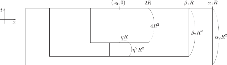
Figure 1. $\alpha_{1}:=\frac{11}{\eta},\,\,\alpha_{2}:=4+\eta^{2}+\frac{\eta^{4}}{4},\,\,\beta_{1}:=\frac{9}{\eta},\,\,\beta_{2}:=4+\eta^{2}$

Proof.

We consider the parabolic contact set

$${\mathcal{A}}_{a,b}\left(\overline{B}_{R}(z_{0});K_{\alpha_{1}R,\,\alpha_{2}R^{2}}(z_{0},0);u\right)\quad\mbox{ for $\,a:=\frac{2}{R^{2}}\,$ and $\,b:=\frac{12}{\eta^{2}R^{2}},$}$$

which will be denoted by ${\mathcal{A}}$ for simplicity. As in the proof of [KKL, Lemma 3.2], for any $\overline{y}\in B_{R}(z_{0})$, we define

$$w_{\overline{y}}(x,t):=\frac{1}{2}R^{2}u(x,t)+\frac{1}{2}d_{\overline{y}}^{2}(x)-C_{\eta}t,\quad\,C_{\eta}:=\frac{b}{a}=\frac{6}{\eta^{2}}.$$

From the assumption (20), we see that

$$\inf_{K_{2R}(z_{0},0)}w_{\overline{y}}\leq\left(5+\frac{24}{\eta^{2}}\right)R^{2}=:A_{\eta}R^{2},$$

and

$$w_{\overline{y}}\geq\left(6+\frac{24}{\eta^{2}}\right)R^{2}=(A_{\eta}+1)R^{2}\quad\mbox{on}\,\,\,K_{\alpha_{1}R,\,\alpha_{2}R^{2}}(z_{0},0)\backslash K_{\beta_{1}R,\,\beta_{2}R^{2}}(z_{0},0).$$

Then we deduce that for any $\displaystyle\left(\overline{y},\overline{h}\right)\in B_{R}(z_{0})\times\left(A_{\eta}R^{2},(A_{\eta}+1)R^{2}\right)$, there exists a time $\displaystyle\overline{t}\in\left(-\beta_{2}R^{2},0\right)$ such that

$$\overline{h}=\inf_{B_{\alpha_{1}R}(z_{0})\times\left(-\alpha_{2}R^{2},\overline{t}\right]}w_{\overline{y}}\,=\,w_{\overline{y}}\left(\overline{x},\overline{t}\right),$$

where the infimum is achieved at an interior point $\overline{x}\in B_{\beta_{1}R}(z_{0}).$ This means that $(\overline{x},\overline{t})$ is a parabolic contact point, i.e., $(\overline{x},\overline{t})\in{\mathcal{A}}.$ According to Lemma 4.2, we observe that

$$\overline{y}=\exp_{\overline{x}}\left(\frac{1}{2}R^{2}\,\nabla u\left(\overline{x},\overline{t}\right)\right),\quad\mbox{and }\quad\overline{x}\not\in\operatorname{Cut}(\overline{y}).$$

Now, we define the map $\phi:K_{\alpha_{1}R,\,\alpha_{2}R^{2}}(z_{0},0)\to M$ as

$$\phi(x,t):=\exp_{x}\left(\frac{1}{2}R^{2}\nabla u(x,t)\right),$$

and the map $\Phi:K_{\alpha_{1}R,\,\alpha_{2}R^{2}}(z_{0},0)\to M\times{\mathbb{R}}$ as

$$\Phi(x,t):=\left(\phi(x,t),-\frac{1}{2}d^{2}\left(x,\phi(x,t)\right)-\frac{1}{2}R^{2}u(x,t)+C_{\eta}t\right).$$

We also define

$$\tilde{\mathcal{A}}:=\left\{(x,t)\in K_{\beta_{1}R,\,\beta_{2}R^{2}}(z_{0},0)\,:\,\exists y\in B_{R}(z_{0})\,\,\,\mbox{s.t.}\,\,\,\displaystyle w_{y}(x,t)=\inf_{B_{\alpha_{1}R}(z_{0})\times\left(-\alpha_{2}R^{2},t\right]}w_{y}\leq(A_{\eta}+1)R^{2}\,\right\}.$$

According to the argument above, we have proved that for any $(y,s)\in B_{R}(z_{0})\times\left(-(A_{\eta}+1)R^{2},-A_{\eta}R^{2}\right)$, there exists a point $(x,t)\in\tilde{\mathcal{A}}$ such that $(y,s)=\Phi(x,t),$ that is,

$$B_{R}(z_{0})\times\left(-(A_{\eta}+1)R^{2},-A_{\eta}R^{2}\right)\subset\Phi(\tilde{\mathcal{A}}).$$

Thus, the area formula provides

(22) $$|B_{R}(z_{0})|\cdot R^{2}\leq\int_{M\times{\mathbb{R}}}{\mathcal{H}}^{0}\left[\tilde{\mathcal{A}}\cap\Phi^{-1}(y,s)\right]dV(y,s)=\int_{\tilde{\mathcal{A}}}\operatorname{Jac}\Phi(x,t)dV(x,t).$$

We note that

(23) $$\tilde{\mathcal{A}}\subset{\mathcal{A}}\cap K_{\beta_{1}R,\beta_{2}R^{2}}(z_{0},0)\cap\{u\leq M_{\eta}\}$$

for $M_{\eta}:=2(A_{\eta}+1)$ since $\frac{1}{2}R^{2}u(x,t)\leq w_{y}(x,t)\leq(A_{\eta}+1)R^{2}$ for $(x,t)\in\tilde{\mathcal{A}}.$

Next, we claim that for $(x,t)\in{\mathcal{A}},$

(24) $$\begin{split}\operatorname{Jac}\Phi(x,t)&\leq\frac{1}{(n+1)^{n+1}}{\mathscr{S}}^{n+1}\left(2\alpha_{1}\sqrt{{\kappa}}\,R_{0}\right)\left[\left\{\frac{nR^{2}}{2\lambda}\left({\frac{\lambda}{n}\Delta u-\partial_{t}u}\right)+\frac{6n}{\lambda\eta^{2}}+n{\mathscr{H}}\left(2\alpha_{1}\sqrt{{\kappa}}\,R_{0}\right)\right\}^{+}\right]^{n+1}.\end{split}$$

From Lemma 4.2, if $(x,t)\in{\mathcal{A}},$ then we have

$$\frac{R^{2}}{2}\nabla u(x,t)=-d_{y}(x)\nabla d_{y}(x)\quad\mbox{for }\,\,\,y:=\phi(x,t)\in\overline{B}_{R}(z_{0});\quad x\notin\operatorname{Cut}(y),$$

and hence

(25) $$\frac{R^{2}}{2}|\nabla u(x,t)|=d_{y}(x)\leq d(y,z_{0})+d(z_{0},x)\leq R+\alpha_{1}R\leq 2\alpha_{1}R_{0}.$$

Using Lemma 4.4 (with $\tilde{\lambda}=\lambda/n$) and (25), we deduce that for $(x,t)\in{\mathcal{A}},$

$$\begin{split}\displaystyle(n+1)&\operatorname{Jac}\Phi(x,t)^{\frac{1}{n+1}}\\ &\leq{\mathscr{S}}\left(\sqrt{\frac{(n-1)\kappa}{n}}\frac{R^{2}|\nabla u|}{2}\right)\left\{\frac{nR^{2}}{2\lambda}\left({\frac{\lambda}{n}\Delta u-\partial_{t}u}\right)+\frac{6n}{\lambda\eta^{2}}+n{\mathscr{H}}\left(\sqrt{\frac{(n-1)\kappa}{n}}\frac{R^{2}|\nabla u|}{2}\right)\right\}^{+}\\ &\leq{\mathscr{S}}\left(2\alpha_{1}\sqrt{{\kappa}}\,R_{0}\right)\left\{\frac{nR^{2}}{2\lambda}\left({\frac{\lambda}{n}\Delta u-\partial_{t}u}\right)+\frac{6n}{\lambda\eta^{2}}+n{\mathscr{H}}\left(2\alpha_{1}\sqrt{{\kappa}}\,R_{0}\right)\right\}^{+},\end{split}$$

since ${\mathscr{H}}(\tau)$ and ${\mathscr{S}}(\tau)$ are nondecreasing for $\tau\geq 0.$ This proves (24).

Lastly, we shall show that for $(x,t)\in{\mathcal{A}},$

(26) $$\frac{\lambda}{n}\Delta u\leq{\mathcal{M}}^{-}(D^{2}u)+\frac{2n\Lambda}{R^{2}}{\mathscr{H}}\left(2\alpha_{1}\sqrt{\kappa}\,R_{0}\right).$$

Indeed, for $(x,t)\in{\mathcal{A}},$ we recall Lemma 4.2 again to see

$$D^{2}\left(u+\frac{1}{R^{2}}d_{y}^{2}\right)(x,t)\geq 0\quad\mbox{ for $y:=\phi(x,t)$};\quad x\notin\operatorname{Cut}(y),$$

i.e., the Hessian of $R^{2}u+d_{y}^{2}$ at $(x,t)$ is positive semidefinite. From Lemma 2.7 and (25), it follows that

$$D^{2}u(x,t)\geq-\frac{2}{R^{2}}D^{2}\left(\frac{1}{2}d_{y}^{2}\right)(x)\geq-\frac{2}{R^{2}}{\mathscr{H}}\left(\sqrt{\kappa}\,d_{y}(x)\right)\,g_{x}\geq-\frac{2}{R^{2}}{\mathscr{H}}\left(2\alpha_{1}\sqrt{\kappa}\,R_{0}\right)g_{x}.$$

Let $\mu_{1}$ be the largest eigenvalue of $D^{2}u(x,t).$ If $\mu_{1}\geq 0,$ then we have

$${\mathcal{M}}^{-}(D^{2}u(x,t)) \geq\lambda\mu_{1}-(n-1)\Lambda\frac{2}{R^{2}}{\mathscr{H}}\left(2\alpha_{1}\sqrt{\kappa}R_{0}\right)$$

$$\geq\frac{\lambda}{n}\Delta u-n\Lambda\frac{2}{R^{2}}{\mathscr{H}}\left(2\alpha_{1}\sqrt{\kappa}R_{0}\right).$$

If $\mu_{1}<0,$ then we have

$${\mathcal{M}}^{-}(D^{2}u(x,t))=\Lambda\Delta u \geq-n\Lambda\frac{2}{R^{2}}{\mathscr{H}}\left(2\alpha_{1}\sqrt{\kappa}R_{0}\right)\geq\frac{\lambda}{n}\Delta u-n\Lambda\frac{2}{R^{2}}{\mathscr{H}}\left(2\alpha_{1}\sqrt{\kappa}R_{0}\right),$$

which proves (26) for $(x,t)\in{\mathcal{A}}.$ Therefore, the ABP-Krylov-Tso type estimate (21) follows from (22), (23) (24) and (26). ∎

As in [KKL], we modify the barrier function of [W] to construct a barrier function in the Riemannian setting. First, we fix some constants that will be used frequently (see Figure 1); for a given $0<\eta<1$,

$$\alpha_{1}:=\frac{11}{\eta},\,\alpha_{2}:=4+\eta^{2}+\frac{\eta^{4}}{4},\,\beta_{1}:=\frac{9}{\eta}\,\,\,\,\mbox{and}\,\,\,\beta_{2}:=4+\eta^{2}.$$

Lemma 4.7.

Assume that

$$\operatorname{Sec}\geq-\kappa\quad\mbox{on $M,$}\quad\mbox{for $\kappa\geq 0.$}$$

Let $R_{0}>0$ and $0<\eta<1$. For $z_{0}\in M,$ and $0<R\leq R_{0},$ there exists a continuous function $v_{\eta}(x,t)$ in $\displaystyle K_{\alpha_{1}R,\,\alpha_{2}R^{2}}(z_{0},\beta_{2}R^{2})$, which is smooth in $\left(M\backslash\operatorname{Cut}(z_{0})\right)\cap K_{\alpha_{1}R,\,\alpha_{2}R^{2}}(z_{0},\beta_{2}R^{2}),$ such that

1. $v_{\eta}(x,t)\geq 0$ in $K_{\alpha_{1}R,\,\alpha_{2}R^{2}}(z_{0},\beta_{2}R^{2})\,\backslash\,K_{\beta_{1}R,\,\beta_{2}R^{2}}(z_{0},\beta_{2}R^{2})$,

2. $v_{\eta}(x,t)\leq 0$ in $K_{2R}(z_{0},\beta_{2}R^{2})$,

3. $R^{2}\left\{{\mathcal{M}}^{+}(D^{2}v_{\eta})-\partial_{t}v_{\eta}\right\}+\frac{12}{\eta^{2}}+2(n+1)\Lambda{\mathscr{H}}\left(2\alpha_{1}\sqrt{\kappa}\,R_{0}\right)\leq 0$ a.e. in $K_{\beta_{1}R,\,\beta_{2}R^{2}}(z_{0},\beta_{2}R^{2})\backslash K_{\frac{\eta}{2}R}(z_{0},\frac{\eta^{2}}{4}R^{2}),$

4. $R^{2}\left\{{\mathcal{M}}^{+}(D^{2}v_{\eta})-\partial_{t}v_{\eta}\right\}\leq C_{\eta}\quad a.e.$ in $K_{\beta_{1}R,\,\beta_{2}R^{2}}(z_{0},\beta_{2}R^{2})$,

5. $v_{\eta}(x,t)\geq-C_{\eta}$ in $K_{\alpha_{1}R,\,\alpha_{2}R^{2}}(z_{0},\beta_{2}R^{2})$,

where ${\mathscr{H}}(\tau)=\tau\coth(\tau),$ and the constant $C_{\eta}>0$ depends only on $\eta,n,\lambda,\Lambda,\sqrt{\kappa}R_{0}$ (independent of $R$ and $z_{0}$).

Proof.

As in [W, Lemma 3.22] and [KKL, Lemma 4.1], we consider

$$h(s,t):=-Ae^{-mt}\left(1-\frac{s}{\beta_{1}^{2}}\right)^{l}\frac{1}{(4\pi t)^{n/2}}\exp\left(-\alpha\frac{s}{t}\right)\quad\mbox{for $t>0$,}$$

and define

$$\varphi_{\eta}(s,t):=h(s,t)+\widetilde{C}t\quad\mbox{in $[0,\beta_{1}^{2}]\times[0,\beta_{2}]\backslash[0,\frac{\eta^{2}}{4}]\times[0,\frac{\eta^{2}}{4}]$, }$$

where $\widetilde{C}:=12/\eta^{2}+2(n+1)\Lambda{\mathscr{H}}\left(2\alpha_{1}\sqrt{\kappa}R_{0}\right),$ and the positive constants $A,m,l,\alpha$ (depending only on $\eta,n,\lambda,\Lambda,\sqrt{\kappa}R_{0}$) will be chosen later. Extending $\varphi_{\eta}$ smoothly in $[0,\alpha_{1}^{2}]\times[-\frac{\eta^{4}}{4},\beta_{2}]$ to satisfy $(a)$ and $(e),$ we define

$$v_{\eta}(x,t):=\varphi_{\eta}\left(\frac{d^{2}_{z_{0}}(x)}{R^{2}},\frac{t}{R^{2}}\right)\quad\mbox{for }\,\,\,\,(x,t)\in K_{\alpha_{1}R,\,\alpha_{2}R^{2}}(z_{0},\beta_{2}R^{2}),$$

where $d_{z_{0}}$ is the distance function to $z_{0}.$ We may assume that $\varphi_{\eta}(s,t)$ is nondecreasing with respect to $s$ in $[0,\alpha_{1}^{2}]\times[-\frac{\eta^{4}}{4},\beta_{2}].$

We recall that

$$\left\langle D^{2}\left(d_{z_{0}}^{2}/2\right)(x)\cdot\xi,\xi\right\rangle=\left\langle d_{z_{0}}D^{2}d_{z_{0}}(x)\cdot\xi,\xi\right\rangle+\left\langle\nabla d_{z_{0}}(x),\xi\right\rangle^{2},\quad\forall\xi\in T_{x}M,\,\,\,x\not\in\operatorname{Cut}(z_{0}),$$

and

$${\mathcal{M}}^{+}\left(D^{2}\left(d_{z_{0}}^{2}/2\right)(x)\right)\leq n\Lambda{\mathscr{H}}\left(\sqrt{\kappa}d_{z_{0}}(x)\right)\leq n\Lambda{\mathscr{H}}\left(\alpha_{1}\sqrt{\kappa}R_{0}\right),\quad\forall x\in B_{\beta_{1}R}(z_{0})\backslash\operatorname{Cut}(z_{0}),$$

from Lemma 2.7. Following the proof of [KKL, Lemma 4.1], and using Lemma 2.15 $(a),$ we can select positive constants $A,m,l,\alpha$, depending only on $\eta,n,\lambda,\Lambda,\sqrt{\kappa}R_{0},$ such that $(b),(c),$ and $(d)$ hold. For the details, we refer to the proof of [KKL, Lemma 4.1] (see also [W, Lemma 3.22]). ∎

We approximate the barrier function $v_{\eta}$ by a sequence of smooth functions as Cabré’s approach in [Ca] since $v_{\eta}(x,t)=\varphi_{\eta}\left(\frac{d_{z_{0}}^{2}(x)}{R^{2}},\frac{t}{R^{2}}\right)$ is not smooth on $\operatorname{Cut}(z_{0}).$ We note that the cut locus of $z_{0}$ is closed and has measure zero. It is not hard to verify the following lemma, and refer to [Ca, Lemmas 5.3, 5.4] for the elliptic case.

Lemma 4.8.

Let $z_{0}\in M,\,R>0$ and let $\varphi:{\mathbb{R}}^{+}\times[0,T]\to{\mathbb{R}}$ be a smooth function such that $\varphi(s,t)$ is nondecreasing with respect to $s$ for any $t\in[0,T]$. Let $v(x,t):=\varphi\left({d^{2}_{z_{0}}(x)},t\right)$. Then there exist a smooth function $\psi$ on $M$ satisfying

$$0\leq\psi\leq 1\quad\mbox{on $M,$}\quad\psi\equiv 1\quad\mbox{in $B_{\beta_{1}R}(z_{0}),$\quad and }\quad\operatorname{supp}\psi\subset B_{\frac{10}{\eta}R}(z_{0}),$$

and a sequence $\{w_{k}\}_{k=1}^{\infty}$ of smooth functions in $M\times[0,T]$ such that

$$\left\{\begin{array}[]{ll}w_{k}\to\psi v&\mbox{uniformly in $M\times[0,T]$, }\\ \partial_{t}w_{k}\to\psi\partial_{t}v&\mbox{uniformly in $M\times[0,T]$, }\\ D^{2}w_{k}\leq Cg_{x}&\mbox{in $M\times[0,T]$, }\\ D^{2}w_{k}\to D^{2}v&\mbox{a.e. in $B_{\beta_{1}R}(z_{0})\times[0,T]$, }\end{array}\right.\qquad\qquad$$

where the constant $C>0$ is independent of $k$.

The following measure estimate of the sublevel set is obtained by applying Lemma 4.6 to $u+v_{\eta}$ with $v_{\eta},$ constructed in Lemma 4.7 and translated in time, with the help of the approximation lemma above.

Proposition 4.9.

Assume that

$$\operatorname{Sec}\geq-\kappa\quad\mbox{on $M$},\quad\mbox{for $\kappa\geq 0,$}$$

and that $F$ satisfies (H1) with $F(0)=0.$ Let $0<\eta<1,$ $0<R\leq R_{0},$ and $K_{\alpha_{1}R,\,\alpha_{2}R^{2}}(z_{0},4R^{2})\subset K_{R_{0}}(x_{0},t_{0})\subset M\times{\mathbb{R}}.$ Let $u$ be a smooth function on $K_{\alpha_{1}R,\,\alpha_{2}R^{2}}(z_{0},4R^{2})$ such that

$$F(D^{2}u)-\partial_{t}u\leq f\quad\mbox{in}\quad K_{\beta_{1}R,\,\beta_{2}R^{2}}(z_{0},4R^{2}),$$

$$u\geq 0\quad\mbox{in}\quad K_{\alpha_{1}R,\,\alpha_{2}R^{2}}(z_{0},4R^{2})\backslash K_{\beta_{1}R,\,\beta_{2}R^{2}}(z_{0},4R^{2}),$$

and

$$\inf_{K_{2R}(z_{0},4R^{2})}u\leq 1.$$

Then, there exist uniform constants $M_{\eta}>1,0<\mu_{\eta}<1$, and $0<\epsilon_{\eta}<1$ such that

$$\frac{\left|\left\{u\leq M_{\eta}\right\}\cap K_{\eta R}(z_{0},0)\right|}{\left|K_{\beta_{1}R,\,\beta_{2}R^{2}}(z_{0},4R^{2})\right|}\geq\mu_{\eta},$$

provided

$$\left(\fint_{K_{\beta_{1}R,\,\beta_{2}R^{2}}(z_{0},4R^{2})}\left|\beta_{1}^{2}R^{2}f^{+}\right|^{n\theta+1}\right)^{\frac{1}{n\theta+1}}\leq\epsilon_{\eta};\quad f^{+}:=\max(f,0),$$

where $\theta:=1+\log_{2}\cosh(4\sqrt{\kappa}R_{0}),$ and $M_{\eta}>0,\,0<\mu_{\eta},\epsilon_{\eta}<1$ depend only on $\eta,n,\lambda,\Lambda$ and $\sqrt{\kappa}R_{0}.$

Proof.

Let $v_{\eta}$ be the barrier function as in Lemma 4.7 after translation in time (by $-\eta^{2}R^{2}$) and let $\{w_{k}\}_{k=1}^{\infty}$ be a sequence of smooth functions approximating $v_{\eta}$ from Lemma 4.8. We notice that $u+v_{\eta}\geq 0$ in $K_{\alpha_{1}R,\,\alpha_{2}R^{2}}(z_{0},4R^{2})\backslash K_{\beta_{1}R,\,\beta_{2}R^{2}}(z_{0},4R^{2})$ and $\displaystyle\inf_{K_{2R}(z_{0},4R^{2})}(u+v_{\eta})\leq 1$. We can apply Lemma 4.6 to $u+w_{k}$ after a slight modification as in the proof of [KKL, Lemma 4.3], and use the dominated convergence theorem to let $k$ go to $+\infty$ due to Lemma 4.8. Thus we obtain

$$|B_{R}(z_{0})|\cdot R^{2}\leq C_{1}\int_{\{u+v_{\eta}\leq M_{\eta}\}\cap K_{\beta_{1}R,\beta_{2}R^{2}}(z_{0},4R^{2})}\left[\left\{R^{2}\left\{{\mathcal{M}}^{-}(D^{2}u+D^{2}v_{\eta})-\partial_{t}(u+v_{\eta})\right\}+C_{2}\right\}^{+}\right]^{n+1},$$

where $C_{1}:={\mathscr{S}}^{n+1}\left(2\sqrt{\kappa}R_{0}\right)/(2\lambda)^{n+1},\,\,$ and $C_{2}:=12/\eta^{2}+2(n+1)\Lambda{\mathscr{H}}\left(2\sqrt{\kappa}\,R_{0}\right).$ Using Lemma 2.15, (H1’) and the properties $(c),(d)$ of $v_{\eta}$ in Lemma 4.7, we have

$$|B_{R}(z_{0})|\cdot R^{2} \leq C_{1}\int_{E_{1}\cup E_{2}}\left[\left\{R^{2}\left\{{\mathcal{M}}^{-}(D^{2}u)-\partial_{t}u\right\}+R^{2}\left\{{\mathcal{M}}^{+}(D^{2}v_{\eta})-\partial_{t}v_{\eta}\right\}+C_{2}\right\}^{+}\right]^{n+1}$$

$$\leq C_{1}\int_{E_{1}\cup E_{2}}\left[\left\{R^{2}\left\{F(D^{2}u)-\partial_{t}u\right\}+R^{2}\left\{{\mathcal{M}}^{+}(D^{2}v_{\eta})-\partial_{t}v_{\eta}\right\}+C_{2}\right\}^{+}\right]^{n+1}$$

$$\leq C_{1}\int_{K_{\beta_{1}R,\,\beta_{2}R^{2}}(z_{0},4R^{2})}\left|R^{2}f^{+}+(C_{\eta}+C_{2})\,\chi_{E_{2}}\right|^{n+1},$$

where $E_{1}:=\{u+v_{\eta}\leq M_{\eta}\}\cap\left(K_{\beta_{1}R,\,\beta_{2}R^{2}}(z_{0},4R^{2})\backslash K_{\eta R}(z_{0},0)\right)$ and $E_{2}:=\{u+v_{\eta}\leq M_{\eta}\}\cap K_{\eta R}(z_{0},0)$. Then, it follows that

$$\frac{|B_{R}(z_{0})|\cdot R^{2}}{\left|K_{\beta_{1}R,\,\beta_{2}R^{2}}(z_{0},4R^{2})\right|} \leq C_{3}\fint_{K_{\beta_{1}R,\,\beta_{2}R^{2}}(z_{0},4R^{2})}\left|\beta_{1}^{2}R^{2}f^{+}+\chi_{E_{2}}\right|^{n+1}$$

$$\leq C_{3}\left(\fint_{K_{\beta_{1}R,\,\beta_{2}R^{2}}(z_{0},4R^{2})}\left|\beta_{1}^{2}R^{2}f^{+}\right|^{n\theta+1}\right)^{\frac{n+1}{n\theta+1}}+C_{3}\frac{\left|E_{2}\right|^{\frac{n+1}{n\theta+1}}}{{\left|K_{\beta_{1}R,\,\beta_{2}R^{2}}(z_{0},4R^{2})\right|^{\frac{n+1}{n\theta+1}}}}$$

for $\theta:=1+\log_{2}\cosh(4\sqrt{\kappa}R_{0})\geq 1,$ where a uniform constant $C_{3}>0$ depending only on $\eta,n,\lambda,\Lambda$ and $\sqrt{\kappa}R_{0}$ may change from line to line. Therefore, Bishop-Gromov’s Theorem 2.3 implies that

$$\frac{\left|E_{2}\right|^{\frac{n+1}{n\theta+1}}}{{\left|K_{\beta_{1}R,\,\beta_{2}R^{2}}(z_{0},4R^{2})\right|^{\frac{n+1}{n\theta+1}}}}+\left(\fint_{K_{\beta_{1}R,\,\beta_{2}R^{2}}(z_{0},4R^{2})}\left|\beta_{1}^{2}R^{2}f^{+}\right|^{n\theta+1}\right)^{\frac{n+1}{n\theta+1}} \geq\frac{1}{C_{3}}\frac{|B_{R}(z_{0})|\cdot R^{2}}{\left|K_{\beta_{1}R,\,\beta_{2}R^{2}}(z_{0},4R^{2})\right|}$$

$$\geq\frac{1}{C_{3}}\frac{1}{{\mathcal{D}}}\left(\frac{1}{\beta_{1}}\right)^{\log_{2}{\mathcal{D}}}\frac{1}{\beta_{2}}=:2\mu_{\eta}^{\frac{n+1}{n\theta+1}}$$

for ${\mathcal{D}}:=2^{n}\cosh^{n-1}(2\sqrt{\kappa}R_{0}).$ By selecting $\epsilon_{\eta}:=\mu_{\eta}^{\frac{1}{n\theta+1}},$ we conclude that

$$\mu_{\eta}\leq\frac{\left|\left\{u+v_{\eta}\leq M_{\eta}\right\}\cap K_{\eta R}(z_{0},0)\right|}{\left|K_{\beta_{1}R,\,\beta_{2}R^{2}}(z_{0},4R^{2})\right|}\leq\frac{\left|\left\{u\leq\tilde{M}_{\eta}\right\}\cap K_{\eta R}(z_{0},0)\right|}{\left|K_{\beta_{1}R,\,\beta_{2}R^{2}}(z_{0},4R^{2})\right|}$$

for $\tilde{M}_{\eta}:=M_{\eta}+C_{\eta}$ depending only on $\eta,n,\lambda,\Lambda$ and $\sqrt{\kappa}R_{0}$ since $v_{\eta}\geq-C_{\eta}$ in $K_{\beta_{1}R,\,\beta_{2}R^{2}}(z_{0},4R^{2})$ from Lemma 4.7. ∎

Remark 4.10.

Let $n,\lambda,\Lambda,$ and $\eta\in(0,1)$ be given, where $\eta$ is fixed as a universal constant in the sequel. Constructing the barrier function in Lemma 4.7, we have chosen a uniform constant $C_{\eta}=C_{\eta}\left(\sqrt{\kappa}R_{0}\right)$ such that

$$C_{\eta}\left(\sqrt{\kappa}R_{0}\right)\gtrsim\exp\left(c\left(1+\sqrt{\kappa}R_{0}\right)^{2}\right),$$

for large $\sqrt{\kappa}R_{0},$ where $c>0$ is a universal constant and we notice that ${\mathscr{H}}(\tau)\leq 1+\tau$ for $\tau\geq 0.$ Due to this choice of $C_{\eta}\left(\sqrt{\kappa}R_{0}\right),$ the positive constants $M_{\eta}\left(\sqrt{\kappa}R_{0}\right),\mu_{\eta}\left(\sqrt{\kappa}R_{0}\right),$ $\epsilon_{\eta}\left(\sqrt{\kappa}R_{0}\right)$ in Proposition 4.9 have been selected so that for large $\sqrt{\kappa}R_{0}>1,$

$$M_{\eta}\left(\sqrt{\kappa}R_{0}\right)\gtrsim\exp\left(c\left(1+\sqrt{\kappa}R_{0}\right)^{2}\right),$$

$$\mu_{\eta}\left(\sqrt{\kappa}R_{0}\right)\lesssim\exp\left(-c\left(1+\sqrt{\kappa}R_{0}\right)^{3}\right)$$

and

$$\epsilon_{\eta}\left(\sqrt{\kappa}R_{0}\right)\lesssim\exp\left(-c\left(1+\sqrt{\kappa}R_{0}\right)^{2}\right).$$

Once Proposition 4.9 is established, a priori Harnack estimate follows from the same procedure as in [KKL] using Bishop and Gromov’s volume comparison theorem. Thus an examination of the procedure asserts that the uniform constant $C_{H}=C_{H}\left(\sqrt{\kappa}R_{0}\right)$ in Theorems 1.2 and 1.3 grows faster than $\exp\left(1+{\kappa}R_{0}^{2}\right)$ as $\sqrt{\kappa}R_{0}\to+\infty$. In fact, $C_{H}(\sqrt{\kappa}R_{0})$ behaves like the exponential composed with a polynomial. It is a rough Harnack estimate compared to the results of [Y1, Y2, BQ] which obtained differential Haranck estimates for the heat equation on a Rimannian manifold $M$ with Ricci curvature bounded by $-\kappa$ ($\kappa\geq 0$) along the line of Li and Yau [LY]. A sharp Li-Yau type Harnack inequality for the heat equation on such a manifold [LX] states that for any $x_{1},x_{2}\in M$ and $0<t_{1}<t_{2}<+\infty$

$$u(x_{1},t_{1})\leq u(x_{2},t_{2})\left(\frac{t_{2}}{t_{1}}\right)^{\frac{n}{2}}\exp\left(\frac{d^{2}(x_{2},x_{1})}{4(t_{2}-t_{1})}\left(1+\frac{1}{3}\kappa(t_{2}+t_{1})\right)+\frac{n}{4}\kappa(t_{2}-t_{1})\right),$$

from which a sharp Haranck constant $C_{H}(\sqrt{\kappa}R_{0})$ for the heat equation has asymptotic growth rate of $\exp\left(1+{\kappa}R_{0}^{2}\right)$ as $\sqrt{\kappa}R_{0}$ tends to infinity.

4.2. Parabolic Harnack inequalities for viscosity solutions

Now we prove Proposition 4.11 which is a counterpart of Proposition 4.9 for viscosity solutions, and a key ingredient in proving Theorems 1.2 and 1.3.

Proposition 4.11.

Assume that

$$\operatorname{Sec}\geq-\kappa\quad\mbox{on $M,$}\quad\mbox{for $\kappa\geq 0,$}$$

and that $F$ satisfies (H1) with $F(0)=0.$ Let $0<\eta<1,$ $0<R\leq R_{0},$ and $K_{\alpha_{1}R,\,\alpha_{2}R^{2}}(z_{0},4R^{2})\subset K_{R_{0}}(x_{0},t_{0})\subset M\times{\mathbb{R}}.$ For $f\in C\left(K_{R_{0}}(x_{0},t_{0})\right),$ let $u\in C\left(K_{R_{0}}(x_{0},t_{0})\right)$ be a viscosity supersolution of

$$F(D^{2}u)-\partial_{t}u=f\quad\mbox{in}\,\,\,\,K_{\alpha_{1}R,\,\alpha_{2}R^{2}}(z_{0},4R^{2}),$$

such that

$$u\geq 0\quad\mbox{in}\quad K_{\alpha_{1}R,\,\alpha_{2}R^{2}}(z_{0},4R^{2})\backslash K_{\beta_{1}R,\,\beta_{2}R^{2}}(z_{0},4R^{2}),$$

and

$$\inf_{K_{2R}(z_{0},4R^{2})}u\leq 1.$$

Then, there exist uniform constants $M_{\eta}>1,0<\mu_{\eta}<1$, and $0<\epsilon_{\eta}<1$ such that

$$\frac{\left|\left\{u\leq M_{\eta}\right\}\cap K_{\eta R}(z_{0},0)\right|}{\left|K_{\alpha_{1}R,\,\alpha_{2}R^{2}}(z_{0},4R^{2})\right|}\geq\mu_{\eta},$$

provided

(27) $$\left(\fint_{K_{R_{0}}(x_{0},t_{0})}\left|R_{0}^{2}f^{+}\right|^{n\theta+1}\right)^{\frac{1}{n\theta+1}}\leq\epsilon_{\eta},$$

where $\theta:=1+\log_{2}\cosh(4\sqrt{\kappa}R_{0}),$ and $M_{\eta}>0,\,0<\mu_{\eta},\epsilon_{\eta}<1$ depend only on $\eta,n,\lambda,\Lambda$ and $\sqrt{\kappa}R_{0}.$

Proof.

It suffices to prove the proposition for $F={\mathcal{M}}^{-}$ owing to the uniform ellipticity (H1’). Setting $\tilde{\alpha}_{1}:=(\alpha_{1}+\beta_{1})/2,$ and $\tilde{\alpha}_{2}:=(\alpha_{2}+\beta_{2})/2,$ we define

$$\Omega\times(T_{0},T_{2}]:=K_{\tilde{\alpha}_{1}R,\,\tilde{\alpha}_{2}R^{2}}(z_{0},4R^{2}),\,\,\,\,\mbox{and }\,\,\,\,H\times(T_{1},T_{2}]:=K_{\beta_{1}R,\,\beta_{2}R^{2}}(z_{0},4R^{2}).$$

We note that $u$ and $f$ belong to $C\left(\overline{\Omega}\times[T_{0},T_{2}]\right),$ and we denote by $\omega$ the modulus of continuity of $u$ on $\overline{\Omega}\times[T_{0},T_{2}],$ which is nondecreasing with $\omega(0+)=0.$

For $\varepsilon>0,$ let $u_{\varepsilon}$ be the inf-convolution of $u$ with respect to $\Omega\times(T_{0},T_{2}]$ as in (9). According to Lemma 3.6, there exists $\varepsilon_{0}>0$ such that if $0<\varepsilon<\varepsilon_{0},$ then $u_{\varepsilon}$ satisfies

$${\mathcal{M}}^{-}(D^{2}u_{\varepsilon})-\partial_{t}u_{\varepsilon}\leq f_{\varepsilon}\quad\mbox{ \,a.e. in $\,\,K_{\beta_{1}R,\,\beta_{2}R^{2}}(z_{0},4R^{2}),$}$$

where $f_{\varepsilon}$ is defined as follows: for $(x,t)\in K_{\beta_{1}R,\,\beta_{2}R^{2}}(z_{0},4R^{2}),$

$$f_{\varepsilon}(x,t):=\sup_{\overline{B}_{2\sqrt{m\varepsilon}}(x)\times\left[t-2\sqrt{m\varepsilon},\min\left\{t+2\sqrt{m\varepsilon},T_{2}\right\}\right]}f+2n\Lambda{\color[rgb]{0,0,0}\kappa\,\omega}\left(2\sqrt{m\varepsilon}\right);\,\,m:=||u||_{L^{\infty}\left(\overline{K}_{\tilde{\alpha}_{1}R,\,\tilde{\alpha}_{2}R^{2}}(z_{0},4R^{2})\right)},$$

and we recall that ${\mathcal{M}}^{-}$ is intrinsically uniformly continuous with respect to $x$ with $\omega_{{\mathcal{M}}^{-}}\equiv 0.$ Using (8) and (27), we have that

$$\begin{array}[]{ll}\left(\fint_{K_{\beta_{1}R,\,\beta_{2}R^{2}}(z_{0},4R^{2})}\left|\beta_{1}^{2}R^{2}f^{+}\right|^{n\theta+1}\right)^{\frac{1}{n\theta+1}}&\leq 2\left(\frac{\beta_{2}}{\beta_{1}^{2}}\right)^{-\frac{1}{n\theta+1}}\left(\fint_{K_{R_{0}}(x_{0},t_{0})}|R_{0}^{2}f^{+}|^{n\theta+1}\right)^{\frac{1}{n\theta+1}}\\ &\leq 2\left(\frac{\beta_{2}}{\beta_{1}^{2}}\right)^{-\frac{1}{n\theta+1}}\epsilon_{\eta}\leq 2\left(\frac{\beta_{2}}{\beta_{1}^{2}}\right)^{-\frac{1}{n+1}}\epsilon_{\eta}=:\tilde{\epsilon}_{\eta},\end{array}$$

and hence for small $\varepsilon>0,$

(28) $$\begin{array}[]{ll}\left(\fint_{K_{\beta_{1}R,\,\beta_{2}R^{2}}(z_{0},4R^{2})}\left|\beta_{1}^{2}R^{2}\left\{{\mathcal{M}}^{-}(D^{2}u_{\varepsilon})-\partial_{t}u_{\varepsilon}\right\}^{+}\right|^{n\theta+1}\right)^{\frac{1}{n\theta+1}}&\leq\left(\fint_{K_{\beta_{1}R,\,\beta_{2}R^{2}}(z_{0},4R^{2})}\left|\beta_{1}^{2}R^{2}f_{\varepsilon}^{+}\right|^{n\theta+1}\right)^{\frac{1}{n\theta+1}}\\ &\leq 2\tilde{\epsilon}_{\eta},\end{array}$$

since $f_{\varepsilon}$ converges uniformly to $f$ in $K_{\beta_{1}R,\,\beta_{2}R^{2}}(z_{0},4R^{2}).$ For a fixed $\delta>0,$ we may assume that for small $\varepsilon>0,$

$$u_{\varepsilon}\geq-\delta\quad\mbox{in}\quad K_{\tilde{\alpha}_{1}R,\,\tilde{\alpha}_{2}R^{2}}(z_{0},4R^{2})\backslash K_{\beta_{1}R,\,\beta_{2}R^{2}}(z_{0},4R^{2}),$$

and

$$\inf_{K_{2R}(z_{0},4R^{2})}u_{\varepsilon}\leq 1+\delta$$

since $u_{\varepsilon}$ converges uniformly to $u$ in $K_{\tilde{\alpha}_{1}R,\,\tilde{\alpha}_{2}R^{2}}(z_{0},4R^{2})$ from Lemma 3.1.

Now, we fix a small $\varepsilon>0.$ According to Lemma 3.2, $(c),$ there is a smooth function $\psi$ on $M\times(-\infty,T_{2}]$ satisfying $0\leq\psi\leq 1$ on $M\times(-\infty,T_{2}]$,

$$\psi\equiv 1\quad\mbox{in $\overline{K}_{\beta_{1}R,\,\beta_{2}R^{2}}(z_{0},4R^{2}),\quad$ and }\quad\operatorname{supp}\psi\subset K_{\tilde{\alpha}_{1}R,\,\tilde{\alpha}_{2}R^{2}}(z_{0},4R^{2}),$$

and we find a sequence $\{w_{k}\}_{k=1}^{\infty}$ of smooth functions on $M\times(-\infty,T_{2}]$ satisfying

$$\left\{\begin{array}[]{ll}w_{k}\to\psi u_{\varepsilon}&\mbox{uniformly in $M\times(-\infty,T_{2}]$ as $k\to+\infty,$}\\ |\nabla w_{k}|+|\partial_{t}w_{k}|\leq C&\mbox{in $M\times(-\infty,T_{2}]$, }\\ \partial_{t}w_{k}\to\partial_{t}u_{\varepsilon}&\mbox{a.e. in $K_{\beta_{1}R,\,\beta_{2}R^{2}}(z_{0},4R^{2})$ as $k\to+\infty,$}\\ D^{2}w_{k}\leq Cg&\mbox{in $M\times(-\infty,T_{2}]$, }\\ D^{2}w_{k}\to D^{2}u_{\varepsilon}&\mbox{a.e. in $K_{\beta_{1}R,\,\beta_{2}R^{2}}(z_{0},4R^{2})$ as $k\to+\infty,$}\\ \end{array}\right.\qquad\qquad$$

where the constant $C>0$ is independent of $k$. For large $k,$ we may assume that

$$w_{k}\geq-2\delta\,\,\,\mbox{in $K_{\alpha_{1}R,\,\alpha_{2}R^{2}}(z_{0},4R^{2})\backslash K_{\beta_{1}R,\,\beta_{2}R^{2}}(z_{0},4R^{2})$},\quad\displaystyle\inf_{K_{2R}(z_{0},4R^{2})}\frac{w_{k}+2\delta}{1+4\delta}\leq 1,$$

and

$$\left(\fint_{K_{\beta_{1}R,\,\beta_{2}R^{2}}(z_{0},4R^{2})}\left|\beta_{1}^{2}R^{2}\left\{{\mathcal{M}}^{-}(D^{2}w_{k})-\partial_{t}w_{k}\right\}^{+}\right|^{n\theta+1}\right)^{\frac{1}{n\theta+1}}\leq 4\tilde{\epsilon}_{\eta},$$

where we used the dominated convergence theorem to obtain the last estimate from (28).

Selecting $\epsilon_{\eta}>0$ small enough, we apply Proposition 4.9 to $\displaystyle\frac{w_{k}+2\delta}{1+4\delta}$ (for large $k$) to obtain

$$\frac{\left|\left\{w_{k}+2\delta\leq(1+4\delta)M_{\eta}\right\}\cap K_{\eta R}(z_{0},0)\right|}{\left|K_{\beta_{1}R,\,\beta_{2}R^{2}}(z_{0},4R^{2})\right|}\geq\mu_{\eta}.$$

By letting $k\to+\infty,$ we have

$$\frac{\left|\left\{u_{\varepsilon}+\delta\leq(1+4\delta)M_{\eta}\right\}\cap K_{\eta R}(z_{0},0)\right|}{\left|K_{\beta_{1}R,\,\beta_{2}R^{2}}(z_{0},4R^{2})\right|}\geq\mu_{\eta}.$$

Since $u_{\varepsilon}$ converges uniformly to $u$ in $K_{\tilde{\alpha}_{1}R,\,\tilde{\alpha}_{2}R^{2}}(z_{0},4R^{2}),$ we let $\varepsilon\to 0$ and $\delta\to 0,$ and use Bishop-Gromov’s Theorem 2.3 to deduce that

$$\frac{\left|\left\{u\leq M_{\eta}\right\}\cap K_{\eta R}(z_{0},0)\right|}{\left|K_{\alpha_{1}R,\,\alpha_{2}R^{2}}(z_{0},4R^{2})\right|}\geq\frac{1}{{\mathcal{D}}}\left(\frac{\beta_{1}}{\alpha_{1}}\right)^{\log_{2}{\mathcal{D}}}\frac{\beta_{2}}{\alpha_{2}}\frac{\left|\left\{u\leq M_{\eta}\right\}\cap K_{\eta R}(z_{0},0)\right|}{\left|K_{\beta_{1}R,\,\beta_{2}R^{2}}(z_{0},4R^{2})\right|}\geq\frac{1}{{\mathcal{D}}}\left(\frac{\beta_{1}}{\alpha_{1}}\right)^{\log_{2}{\mathcal{D}}}\frac{\beta_{2}}{\alpha_{2}}\mu_{\eta}>0$$

for ${\mathcal{D}}:=2^{n}\cosh^{n-1}(4\sqrt{\kappa}R_{0}),$ which finishes the proof. ∎

Sketch of proof of Theorems 1.2 and 1.3

Theorems 1.2 and 1.3 follow from Proposition 4.11 and a standard covering argument using Bishop and Gromov’s Theorem 2.3. Indeed, we first prove a decay estimate for the distribution function of a viscosity supersolution $u$ to ${\mathcal{M}}^{-}(D^{2}u)-\partial_{t}u\leq f^{+}$ in $K_{2R}(x_{0},4R^{2}).$ The main tools of the proof are Proposition 4.11, and a parabolic version of the Calderón-Zygmund decomposition in [Ch] according to Bishop and Gromov’s Theorem 2.3. Then, the weak Harnack inequality in Theorem 1.3 follows. To complete the proof of Theorem 1.2 for the viscosity solution $u\in{\mathcal{S}}_{P}^{*}(f)$, we apply Proposition 4.11, and obtain the same decay estimate for $w:=C_{1}-C_{2}u$ (for $C_{1},C_{2}>0$), which satisfies

$${\mathcal{M}}^{-}(D^{2}w)-\partial_{t}w=-C_{2}\left\{{\mathcal{M}}^{+}(D^{2}u)-\partial_{t}u\right\}\leq C_{2}|f|$$

in the viscosity sense. For the detailed proofs, we refer to [KKL, W].

5. Elliptic Harnack inequality

Using the sup and inf-convolutions, we will prove Harnack inequalities of continuous viscosity solutions to elliptic equations from a priori estimates. We recall viscosity solutions for uniformly elliptic operators.

Definition 5.1 (Viscosity sub and super-differentials, [AFS]).

Let $\Omega\subset M$ be open and let $u:\Omega\to{\mathbb{R}}$ be a lower semi-continuous function. We define the second order subjet of $u$ at $x\in\Omega$ by

$${\mathcal{J}}^{2,-}u(x):= \left\{\left(\nabla\varphi(x),D^{2}\varphi(x)\right)\in T_{x}M\times\operatorname{Sym}TM_{x}:\varphi\in C^{2}(\Omega),\right.$$

$$\left.u-\varphi\,\,\,\mbox{has a local minimum at $x$}\right\}.$$

If $(\zeta,A)\in{\mathcal{J}}^{2,-}u(x),$ $\zeta$ and $A$ are called a first order subdifferential and a second order subdifferential of $u$ at $x,$ respectively.

Similarly, for a upper semi-continuous function $u:\Omega\to{\mathbb{R}},$ we define the second order superjet of $u$ at $x\in\Omega$ by

$${\mathcal{J}}^{2,+}u(x):= \left\{\left(\nabla\varphi(x),D^{2}\varphi(x)\right)\in T_{x}M\times\operatorname{Sym}TM_{x}:\varphi\in C^{2}(\Omega),\right.$$

$$\left.u-\varphi\,\,\,\mbox{has a local maximum at $x$}\right\}.$$

We quote the following local characterization of ${\mathcal{J}}^{2,-}u$ from [AFS, Proposition 2.2].

Lemma 5.2.

Let $u:\Omega\to{\mathbb{R}}$ be a lower semi-continuous function and $x\in M.$ The following statements are equivalent:

1. $(\zeta,A)\in{\mathcal{J}}^{2,-}u(x).$

2. $u\left(\exp_{x}\xi\right)\geq u(x)+\langle\zeta,\xi\rangle+\frac{1}{2}\langle A\xi,\xi\rangle+o(|\xi|^{2})\,\,$ as $\,\,T_{x}M\owns\xi\to 0.$

Definition 5.3 (Viscosity solution).

(i) Let $F:M\times{\mathbb{R}}\times TM\times\operatorname{Sym}TM\to{\mathbb{R}}$ and let $\Omega\subset M$ be an open set. We say that a upper semi-continuous function $u:\Omega\to{\mathbb{R}}$ is a viscosity subsolution of the equation $F(x,u,\nabla u,D^{2}u)=0$ on $\Omega$ if

$$F\left(x,u(x),\zeta,A\right)\geq 0$$

for any $x\in\Omega$ and $(\zeta,A)\in{\mathcal{J}}^{2,+}u(x).$ Similarly, a lower semi-continuous function $u:\Omega\to{\mathbb{R}}$ is said to be a viscosity supersolution of the equation $F(x,u,\nabla u,D^{2}u)=0$ on $\Omega$ if

$$F\left(x,u(x),\zeta,A\right)\leq 0$$

for any $x\in\Omega$ and $(\zeta,A)\in{\mathcal{J}}^{2,-}u(x).$ We say $u$ is a viscosity solution if $u$ is both a viscosity subsolution and a viscosity supersolution.

(ii) Let $\Omega\subset M$ be open, and let $0<\lambda\leq\Lambda.$ We denote by $\overline{\mathcal{S}}_{E}\left(\lambda,\Lambda,f\right)$ a class of a viscosity supersolution $u\in C(\Omega)$ satisfying

$${\mathcal{M}}^{-}(D^{2}u)\leq f\quad\mbox{in $\Omega$}$$

in the viscosity sense. Similarly, a class $\underline{{\mathcal{S}}}_{E}\left(\lambda,\Lambda,f\right)$ of subsolutions is defined as the set of $u\in C(\Omega)$ such that

$${\mathcal{M}}^{+}(D^{2}u)\geq f\quad\mbox{ in $\Omega$}$$

in the viscosity sense. We also define

$${\mathcal{S}}_{E}^{*}\left(\lambda,\Lambda,f\right):=\overline{\mathcal{S}}_{E}\left(\lambda,\Lambda,|f|\right)\cap\underline{{\mathcal{S}}}_{E}\left(\lambda,\Lambda,-|f|\right).$$

We write shortly $\overline{\mathcal{S}}_{E}(f),\underline{{\mathcal{S}}}_{E}(f),$and ${\mathcal{S}}_{E}^{*}(f)$ for $\overline{\mathcal{S}}_{E}\left(\lambda,\Lambda,f\right),\underline{{\mathcal{S}}}_{E}\left(\lambda,\Lambda,f\right),$ and ${\mathcal{S}}_{E}^{*}\left(\lambda,\Lambda,f\right),$ respectively.

As in the parabolic case, we use the sup and inf-convolutions to approximate continuous viscosity solutions. Let $\Omega\subset M$ be a bounded open set, and $u$ be a continuous function on $\overline{\Omega}.$ For $\varepsilon>0,$ let $u_{\varepsilon}$ denote the inf-convolution of $u$ (with respect to $\Omega$), defined as follows: for $x_{0}\in\overline{\Omega},$

$$u_{\varepsilon}(x_{0}):=\inf_{y\in\overline{\Omega}}\left\{u(y)+\frac{1}{2\varepsilon}d^{2}(y,x_{0})\right\}.$$

If $y_{0}$ is a point to realize the above infimum, then we have

$$u_{\varepsilon}(x_{0})=u(y_{0})+\frac{1}{2\varepsilon}d^{2}(y_{0},x_{0})\leq u(y)+\frac{1}{2\varepsilon}d^{2}(y,x_{0})\quad\forall y\in\Omega,$$

which means $u$ has a touching paraboloid $-\frac{1}{2\varepsilon}d^{2}(y,x_{0})+u(y_{0})+\frac{1}{2\varepsilon}d^{2}(y_{0},x_{0})$ at $y_{0}$ from below.

Now we state the elliptic analogue of the results in Section 3 without proof.

Lemma 5.4.

For $u\in C\left(\overline{\Omega}\right),$ let $u_{\varepsilon}$ be the inf-convolution of $u$ with respect to $\Omega$ and let $x_{0}\in\overline{\Omega}.$

1. If $0<\varepsilon<\varepsilon^{\prime},$ then $u_{\varepsilon^{\prime}}(x_{0})\leq u_{\varepsilon}(x_{0})\leq u(x_{0}).$

2. There exists $\displaystyle\,y_{0}\in\overline{\Omega}$ such that $u_{\varepsilon}(x_{0})=u(y_{0})+\frac{1}{2\varepsilon}d^{2}(y_{0},x_{0}).$

3. $\displaystyle d^{2}(y_{0},x_{0})\leq 2\varepsilon|u(x_{0})-u(y_{0})|\leq 4\varepsilon||u||_{L^{\infty}(\Omega)}.$

4. $u_{\varepsilon}\uparrow u$ uniformly in $\overline{\Omega}.$

5. $u_{\varepsilon}$ is Lipschitz continuous in $\overline{\Omega}$: for $x_{0},x_{1}\in\overline{\Omega},$

   $$|u_{\epsilon}(x_{0})-u_{\varepsilon}(x_{1})|\leq\frac{3}{2\varepsilon}\operatorname{diam}(\Omega)d(x_{0},x_{1}).$$

Lemma 5.5.

Assume that

$$\operatorname{Sec}\geq-\kappa\quad\mbox{on $M,\quad$ for $\kappa\geq 0$.}$$

For $u\in C\left(\overline{\Omega}\right),$ let $u_{\varepsilon}$ be the inf-convolution of $u$ with respect to $\Omega,$ where $\Omega\subset M$ is a bounded open set.

1. $u_{\varepsilon}$ is semi-concave in $\Omega.$ Moreover, for almost every $x\in\Omega,$ $u_{\varepsilon}$ is differentiable at $x,$ and there exists the Hessian $D^{2}u_{\varepsilon}(x)$ (in the sense of Aleksandrov-Bangert’s Theorem 2.8) such that

   $$u_{\varepsilon}\left(\exp_{x}\xi\right)=u_{\varepsilon}(x)+\left\langle\nabla u_{\varepsilon}(x),\xi\right\rangle+\frac{1}{2}{\left\langle A(x)\cdot\xi,\xi\right\rangle}+o\left(|\xi|^{2}\right)$$

   as $\xi\in T_{x}M\to 0.$

2. $\displaystyle D^{2}u_{\varepsilon}(x)\leq\frac{1}{\varepsilon}{\sqrt{\kappa}\operatorname{diam}(\Omega)\coth\left(\sqrt{\kappa}\operatorname{diam}(\Omega)\right)}\,g_{x}\,\,\,$ a.e. in $\Omega.$

3. Let $H$ be an open set such that $\overline{H}\subset\Omega.$ Then, there exist a smooth function $\psi$ on $M$ satisfying

   $$\mbox{$0\leq\psi\leq 1$ on $M$},\,\,\,\,\,\psi\equiv 1\,\,\,\,\mbox{in $\overline{H}\,\,\,\,\,$ and }\,\,\,\,\operatorname{supp}\psi\subset\Omega,$$

   and a sequence $\{w_{k}\}_{k=1}^{\infty}$ of smooth functions on $M$ such that

   $$\left\{\begin{array}[]{ll}w_{k}\to\psi u_{\varepsilon}&\mbox{uniformly in $M\,\,$ as $k\to+\infty,$}\\ |\nabla w_{k}|\leq C&\mbox{in $M$, }\\ D^{2}w_{k}\leq Cg&\mbox{in $M$, }\\ D^{2}w_{k}\to D^{2}u_{\varepsilon}&\mbox{a.e. in $H\,\,$ as $k\to+\infty,$}\\ \end{array}\right.\qquad\qquad$$

   where the constant $C>0$ is independent of $k$.

Proposition 5.6.

Assume that

$$\operatorname{Sec}\geq-\kappa\qquad\mbox{on $M,\qquad$ for $\kappa\geq 0$.}$$

Let $H\subset M$ be a bounded open set such that $\overline{H}\subset\Omega.$ Let $u\in C\left(\overline{\Omega}\right),$ and let $\omega$ denote a modulus of continuity of $u$ on $\overline{\Omega},$ which is nondecreasing on $(0,+\infty)$ with $\omega(0+)=0.$ For $\varepsilon>0,$ let $u_{\varepsilon}$ be the inf-convolution of $u$ with respect to $\Omega.$ Then, there exists $\varepsilon_{0}>0$ depending only on $||u||_{L^{\infty}\left(\overline{\Omega}\right)},H,$ and $\Omega,$ such that if $0<\varepsilon<\varepsilon_{0},$ then the following statements hold: let $x_{0}\in\overline{H},$ and let $y_{0}\in\overline{\Omega}$ satisfy

$$u_{\varepsilon}(x_{0})=u(y_{0})+\frac{1}{2\varepsilon}d^{2}(y_{0},x_{0}).$$

1. We have that $y_{0}\in\Omega,$ and there is a unique minimizing geodesic joining $x_{0}$ to $y_{0}.$

2. If $(\zeta,A)\in{\mathcal{J}}^{2,-}u_{\varepsilon}(x_{0}),$ then we have

   $$y_{0}=\exp_{x_{0}}(-\varepsilon\zeta).$$

3. If $(\zeta,A)\in{\mathcal{J}}^{2,-}u_{\varepsilon}(x_{0}),$ then we have

   $$\left(\,L_{x_{0},y_{0}}\zeta,\,L_{x_{0},y_{0}}\circ A-{\color[rgb]{0,0,0}2\kappa\,\omega\left(2\sqrt{\varepsilon\,||u||_{L^{\infty}\left(\overline{\Omega}\right)}}\right)}\,g_{y_{0}}\right)\,\in{\mathcal{J}}^{2,-}u(y_{0}),$$

   where $L_{x_{0},y_{0}}$ stands for the parallel transport along the unique minimizing geodesic joining $x_{0}$ to $y_{0}=\exp_{x_{0}}(-\varepsilon\zeta).$

Lemma 5.7.

Under the same assumption as Proposition 5.6, we also assume that $F$ satisfies (H1) and (H2). For ${\color[rgb]{0,0,0}f\in C\left(\Omega\right)},$ let $u\in C\left(\overline{\Omega}\right)$ be a viscosity supersolution of

$$F(D^{2}u)=f\quad\mbox{in $\Omega.$}$$

If $0<\varepsilon<\varepsilon_{0},$ then the inf-convolution $u_{\varepsilon}$ (with respect to $\Omega$) is a viscosity supersolution of

$$F(D^{2}u_{\varepsilon})=f_{\varepsilon}\quad\mbox{on $H$},$$

where $\varepsilon_{0}>0$ is the constant as in Proposition 5.6, and

$$f_{\varepsilon}(x):=\sup_{\overline{B}_{2\sqrt{m\varepsilon}}(x)}f+{\color[rgb]{0,0,0}\omega_{F}}\left(2\sqrt{m\varepsilon}\right)+2n\Lambda{\color[rgb]{0,0,0}\kappa\,\omega}\left(2\sqrt{m\varepsilon}\right);\quad m:=||u||_{L^{\infty}\left(\overline{\Omega}\right)}.$$

Moreover, we have

$$F(D^{2}u_{\varepsilon})\leq f_{\varepsilon}\quad\mbox{ a.e. in $H.$}$$

In particular, Lemma 5.7 holds for Pucci’s extremal operators according to Remark 3.5.

The following proposition is quoted from the proof of [WZ, Proposition 4.1], which is a main ingredient in the proof of a priori Harnack estimate.

Proposition 5.8.

Assume that

$$\operatorname{Sec}\geq-\kappa\quad\mbox{on $M,\quad$ for $\kappa\geq 0,$}$$

and $F$ satisfies (H1) with $F(0)=0.$ Let $0<R\leq R_{0}$ and $u$ be a smooth function satisfying $F(D^{2}u)\leq f$ in $B_{2R}(x_{0})\subset M.$ Then, there exist uniform constants $M_{0}>0,0<\mu_{0}<1,$ and $0<\epsilon_{0}<1,$ depending only on $n,\lambda,\Lambda$ and $\sqrt{\kappa}R_{0},$ such that if for any $B_{r}(z_{0})\subset B_{2R}(x_{0}),$

$$u\geq 0\quad\mbox{in $B_{r}(z_{0}),$}\quad\inf_{B_{r/2}(z_{0})}u\leq 1,$$

and

$$\left(\fint_{B_{3r/4}(z_{0})}|r^{2}f^{+}|^{n\theta}\right)^{\frac{1}{n\theta}}\leq\epsilon_{0};\quad f^{+}:=\max(f,0),$$

then we have

$$\frac{\left|\left\{u\leq M_{0}\right\}\cap B_{r/8}(z_{0})\right|}{|B_{r}(z_{0})|}\geq\mu_{0},$$

where $\theta:=1+\log_{2}\cosh\left(8\sqrt{\kappa}R_{0}\right).$

Lemma 5.9.

Assume that

$$\operatorname{Sec}\geq-\kappa\quad\mbox{on $M,\quad$ for $\kappa\geq 0$},$$

and $F$ satisfies (H1) with $F(0)=0.$ Let $0<R\leq R_{0}.$ For $f\in C\left(B_{2R}(x_{0})\right),$ let $u\in C\left(B_{2R}(x_{0})\right)$ be a viscosity supersolution of

$$F(D^{2}u)=f\quad\mbox{ in $B_{2R}(x_{0}).$}$$

Then, there exist uniform constants $M_{0}>0,0<\mu_{0}<1,$ and $0<\epsilon_{0}<1,$ depending only on $n,\lambda,\Lambda$ and $\sqrt{\kappa}R_{0},$ such that if for any $B_{r}(z_{0})\subset B_{2R}(x_{0}),$

$$u\geq 0\quad\mbox{in $B_{r}(z_{0}),$}\quad\mbox{and}\quad\inf_{B_{r/2}(z_{0})}u\leq 1,$$

then we have

$$\frac{\left|\left\{u\leq M_{0}\right\}\cap B_{r/8}(z_{0})\right|}{|B_{r}(z_{0})|}\geq\mu_{0},$$

provided that

$$\left(\fint_{B_{2R}(x_{0})}|R^{2}f^{+}|^{n\theta}\right)^{\frac{1}{n\theta}}\leq\epsilon_{0};\quad f^{+}:=\max(f,0),$$

where $\theta:=1+\log_{2}\cosh\left(8\sqrt{\kappa}R_{0}\right).$

Proof.

It suffices to prove the proposition for $F={\mathcal{M}}^{-}$ from (H1’). Set

$$\Omega:=B_{7r/8}(z_{0}),\quad\mbox{and}\quad H:=B_{3r/4}(z_{0}).$$

We note that $u$ and $f$ belong to $C\left(\overline{\Omega}\right),$ and denote by $\omega$ the modulus of continuity of $u$ on $\overline{\Omega},$ which is nondecreasing with $\omega(0+)=0.$

For small $\varepsilon>0,$ let $u_{\varepsilon}$ be the inf-convolution of $u$ with respect to $\Omega.$ According to Lemma 5.7, we find $\varepsilon_{0}>0$ such that for $0<\varepsilon<\varepsilon_{0},$ $u_{\varepsilon}$ satisfies

$${\mathcal{M}}^{-}(D^{2}u_{\varepsilon})\leq f_{\varepsilon}\quad\mbox{ \,a.e. in $\,\,B_{3r/4}(z_{0}),$}$$

where $f_{\varepsilon}$ is defined as follows: for $x\in B_{3r/4}(z_{0}),$

$$f_{\varepsilon}(x):=\sup_{\overline{B}_{2\sqrt{m\varepsilon}}(x)}f+2n\Lambda{\color[rgb]{0,0,0}\kappa\,\omega}\left(2\sqrt{m\varepsilon}\right);\quad m:=||u||_{L^{\infty}\left(\overline{B}_{7r/8}(z_{0})\right)},$$

and we recall that ${\mathcal{M}}^{-}$ is intrinsically uniformly continuous with respect to $x$ with $\omega_{{\mathcal{M}}^{-}}\equiv 0.$ Using (7), we have that

$$\left(\frac{3r}{4}\right)^{2}\left(\fint_{B_{3r/4}(z_{0})}|f^{+}|^{n\theta}\right)^{\frac{1}{n\theta}}\leq 2\cdot 4R^{2}\left(\fint_{B_{2R}(x_{0})}|f^{+}|^{n\theta}\right)^{\frac{1}{n\theta}}\leq 8\epsilon_{0};\quad\theta:=1+\log_{2}\cosh\left(8\sqrt{\kappa}R_{0}\right),$$

and hence for small $\varepsilon>0,$

(29) $$\left(\frac{3r}{4}\right)^{2}\left(\fint_{B_{3r/4}(z_{0})}\left|\left\{{\mathcal{M}}^{-}(D^{2}u_{\varepsilon})\right\}^{+}\right|^{n\theta}\right)^{\frac{1}{n\theta}}\leq\left(\frac{3r}{4}\right)^{2}\left(\fint_{B_{3r/4}(z_{0})}|f_{\varepsilon}^{+}|^{n\theta}\right)^{\frac{1}{n\theta}}\leq 9\epsilon_{0}$$

since $f_{\varepsilon}$ converges uniformly to $f$ in $B_{3r/4}(z_{0}).$ For a fixed $\delta>0,$ we may assume that for small $\varepsilon>0,$

$$u_{\varepsilon}\geq-\delta\quad\mbox{in}\quad B_{7r/8}(z_{0}),\quad\mbox{and}\quad\displaystyle\inf_{B_{r/2}(z_{0})}u_{\varepsilon}\leq 1+\delta$$

since $u_{\varepsilon}$ converges uniformly to $u$ in $B_{7r/8}(z_{0})$ from Lemma 5.4.

Now, we fix a small $\varepsilon>0.$ According to Lemma 5.5, $(c),$ there is a smooth function $\psi$ such that $0\leq\psi\leq 1$ on $M,$

$$\psi\equiv 1\quad\mbox{in $\overline{B}_{3r/4}(z_{0}),$}\quad\mbox{and}\quad{\operatorname{supp}\psi\subset B_{7r/8}(z_{0})},$$

and we approximate $\psi u_{\varepsilon}$ by smooth functions $w_{k}$ on $M$ satisfying

$$\left\{\begin{array}[]{ll}w_{k}\to\psi u_{\varepsilon}&\mbox{uniformly in $M$ as $k\to+\infty,$}\\ |\nabla w_{k}|\leq C&\mbox{in $M$, }\\ D^{2}w_{k}\leq Cg&\mbox{in $M$, }\\ D^{2}w_{k}\to D^{2}u_{\varepsilon}&\mbox{a.e. in $B_{3r/4}(z_{0})$ as $k\to+\infty,$}\\ \end{array}\right.\qquad\qquad$$

where the constant $C>0$ is independent of $k$. For large $k,$ we may assume that

$$w_{k}\geq-2\delta\,\,\,\mbox{in $B_{r}(z_{0})$}\quad\mbox{and}\quad\displaystyle\inf_{B_{r/2}(z_{0})}w_{k}\leq 1+2\delta,$$

and

$$\left(\frac{3r}{4}\right)^{2}\left(\fint_{B_{3r/4}(z_{0})}\left|\left\{{\mathcal{M}}^{-}(D^{2}w_{k})\right\}^{+}\right|^{n\theta}\right)^{\frac{1}{n\theta}}\leq 10\epsilon_{0},$$

where we used the dominated convergence theorem to obtain the last estimate from (29). By selecting $\epsilon_{0}>0$ small enough, we apply Theorem 5.8 to $\displaystyle\frac{w_{k}+2\delta}{1+4\delta}$ (for large $k$) to obtain that

$$\frac{\left|\left\{w_{k}+2\delta\leq(1+4\delta)M_{0}\right\}\cap B_{r/8}(z_{0})\right|}{|B_{r}(z_{0})|}\geq\mu_{0}.$$

By letting $k\to+\infty,$ we have

$$\frac{\left|\left\{u_{\varepsilon}+\delta\leq(1+4\delta)M_{0}\right\}\cap B_{r/8}(z_{0})\right|}{|B_{r}(z_{0})|}\geq\mu_{0}.$$

Since $u_{\varepsilon}$ converges uniformly to $u$ in $B_{7r/8}(z_{0}),$ we let $\varepsilon\to 0$ and $\delta\to 0$ to conclude that

$$\frac{\left|\left\{u\leq M_{0}\right\}\cap B_{r/8}(z_{0})\right|}{|B_{r}(z_{0})|}\geq\mu_{0}$$

which finishes the proof. ∎

Proof of Theorems 1.4 and 1.5 Theorems 1.4 and 1.5 follow from Lemma 5.9 and a standard covering argument employing Bishop and Gromov’s Theorem 2.3 (see [Ca] for instance). ∎

Acknowledgement Ki-Ahm Lee was supported by Basic Science Research Pro- gram through the National Research Foundation of Korea(NRF) grant funded by the Korea government(MEST)(2010-0001985). Ki-Ahm Lee also hold a joint appointment with the Research Institute of Mathematics of Seoul National University.

References

- [A] A. D. Aleksandrov, Almost everywhere existence of the second differential of a convex function and some properties of convex surfaces connected with it (in Russian), Uchen. Zap. Leningrad. Gos. Univ., Math. Ser. 6 (1939), 3-35.
- [AFS] D. Azagra, J. Ferrera and B. Sanz, Viscosity solutions to second order partial differential equations on Riemannian manifolds, J. Differential Equations 245 (2008), 307-336.
- [BQ] D. Bakry and Z. M. Qian, Harnack inequalities on a manifold with positive or negative Ricci curvature, Revista matemática iberoamericana 15 (1999), 143-179.
- [B] V. Bangert, Analytische Eigenschaften konvexer Funktionen auf Riemannschen Man- nigfaltigkeiten, J. Reine Angew. Math. 307 (1979), 309-324.
- [Ca] X. Cabré, Nondivergent elliptic equations on manifolds with nonnegative curvature, Comm. Pure Appl. Math. 50 (1997), 623-665.
- [CC] L. A. Caffarelli and X. Cabré, Fully Nonlinear Elliptic Equations, American Mathematical Society Colloquium Publications 43, American Mathematical Society, Providence, RI, 1995.
- [Ch] M. Christ, A theorem with remarks on analytic capacity and the Cauchy integral, Colloq. Math. 60/61 (1990), 601-628.
- [CMS] D. Cordero-Erausquin, R. J. McCann and M. Schmuckenschläger, A Riemannian interpolation inequality à la Borell, Brascamp and Lieb. Invent. Math. 146 (2001), 219-257.
- [CIL] M. G. Crandall, H. Ishii and P.-L. Lions, User’s guide to viscosity solutions of second order partial differential equations, Bull. Amer. Math. Soc. 27 (1992), 1-67.
- [D] M. P. do Carmo, Riemannian geometry, Mathematics: Theory & Applications, Birkhaüser Boston Inc., Boston, MA, 1992. Translated from the second Portuguese edition by Francis Flaherty.
- [J] R. Jensen, The Maximum Principle for viscosity solutions of fully nonlinear second order partial differential equations, Arch. Rat. Mech. Anal. 101 (1988), 1-27.
- [JLS] R. Jensen, P.-L. Lions and P.E. Souganidis, A uniqueness result for viscosity solutions of second order fully nonlinear partial differential equations, Proc. Amer. Math. Soc. 102 (1988), 975-978.
- [Ju] P. Juutinen, On the definition of viscosity solutions for parabolic equations, Proc. Amer. Math. Soc. 129 (2001), 2907-2911.
- [K] S. Kim, Harnack inequality for nondivergent elliptic operators on Riemannian manifolds, Pacific J. Math. 213 (2004), 281-293.
- [KKL] S. Kim, S. Kim and K.-A. Lee , Harnack inequality for nondivergent parabolic operators on Riemannian manifolds, Calc. Var. 49 (2014), 669-706.
- [Kr] N. V. Krylov, Sequences of convex functions and estimates of the maximum of the solution of a parabolic equation (Russian), Sibirskii Mat. Zh. 17 (1976), 290-303; Siberian Math. J. 17 (1976), 226-236 (English).
- [KS] N. V. Krylov and M. V. Safonov, A property of the solutions of parabolic equations with measurable coefficients (Russian), Izv. Akad. Nauk SSSR Ser. Mat. 44(1) (1980), 161-175; Math. USSR Izvestija 16 (1981), 151-164 (English).
- [LX] J. F. Li and X. J. Xu, Differential Harnack inequalities on Riemannian manifolds I: linear heat equation, Adv. Math. 226 (2011), 4456-4491.
- [LY] P. Li and. S.-T. Yau, On the parabolic kernel of the Schrödinger operator, Acta Math. 156 (1986), 153-201.
- [PZ] S. Peng and D. Zhou, Maximum principle for viscosity solutions on Riemannian manifolds, arXiv:0806.4768.
- [T] K. Tso, On an Aleksandrov-Bakelman type maximum principle for second-order parabolic equations, Comm. Partial Differential Equations 10 (1985), 543-553.
- [V] C. Villani, Optimal Transport: Old and New, Springer-Verlag, Berlin, 2009.
- [W] L. Wang, On the regularity theory of fully nonlinear parabolic equations. I, Comm. Pure Appl. Math. 45 (1992), 27-76.
- [WZ] Y. Wang and X. Zhang, An Alexandroff-Bakelman-Pucci estimate on Riemannian manifolds, Adv. Math 232 (2013), 499-512.
- [Y1] S.-T. Yau, On the Harnack inequalities for partial differential equations, Comm. Anal. Geom. 2 (1994), 431-450.
- [Y2] S.-T. Yau, Harnack inequality for non-self-adjoint evolution equations, Math. Res. Lett. 2 (1995), 387-399.
- [Z] X. Zhu, Viscosity solutions to second order parabolic PDEs on Riemannian manifolds, Acta Appl. Math. 115 (2011), 279-290.