Extreme value statistics of networks with inhibitory and excitatory couplings

Abstract

Inspired by the importance of inhibitory and excitatory couplings in the brain, we analyze the largest eigenvalue statistics of a random networks incorporating such features. We find that the largest real part of eigenvalues of a network, which accounts for the stability of underlying system, decreases linearly as a function of inhibitory connection probability up to a particular threshold value, after which it exhibits rich behaviors with the distribution manifesting generalized extreme value statistics. Fluctuations in the largest eigenvalue remain somewhat robust against an increase in system size, but reflect a strong dependence on the number of connections indicating that systems having more interactions among its constituents are likely to be more unstable.

I Introduction

The largest eigenvalue of network adjacency matrix appears in many applications. In particular, for dynamic processes on graphs, the inverse of the largest eigenvalue characterizes the threshold of phase transition in both virus spread Mieghem2009 and synchronization of coupled oscillators Restrepo in networks. In neuroscience, networks of neurons are often studied using models in which interconnections are represented by a synaptic matrix with elements drawn randomly Sompolinsky ; Cessac . Eigenvalues of these matrices are useful for studying spontaneous activities and evoked responses in such models Sompolinsky ; Vogels , and the existence of spontaneous activity depends on whether the real part of any eigenvalue is large enough to destabilize the silent state in a linear analysis. Furthermore, the largest real part of the spectra provides strong clues about the nature of spontaneous activity in nonlinear models Rajan . A recent work reveals the importance of the largest eigenvalue in determining disease spread in complex networks, where epidemic threshold relates with inverse of the largest eigenvalue Mendes2012 . In context of ecological systems, a celebrated work by Robert May demonstrates that largest real part of eigenvalue of corresponding adjacency matrix contains information about stability of underlying system MayNature1972 . Mathematically, matrices satisfying a set of constraints are stable Quirck1965 . But most real world systems have underlying interaction matrix which are too complicated to satisfy these constraints and hence, study of fluctuations in largest real part of eigenvalues is crucial to understand stability of a system, as well as of an individual network in that ensemble.

Largest eigenvalues over ensembles of random Hermitian matrices yielding correlated eigenvalues follow Tracy-Widom distribution Tracy . Whereas, extreme value statistics for independent identically distributed random variables can be formulated entirely in terms of three universal types of probability functions: the Fréchet, Gumbel and Weibull known as generalized extreme value (GEV) statistics depending upon whether the tail of the density is respectively power-law, faster than any power-law, and bounded or unbounded book_gev . The GEV statistics with location parameter $\mu$, scale parameter $\sigma$ and shape parameter $\xi$ has often been used to model unnormalized data from a given system. Probability density function for extreme value statistics with these parameters is given by book_gev

$$\rho(x)=\begin{cases}\frac{1}{\sigma}\big{[}1+\big{(}\xi\frac{(x-\mu)}{\sigma}\big{)}^{-1-\frac{1}{\xi}}\big{]}\exp\big{[}-\big{(}1+\big{(}\xi\frac{(x-\mu)}{\sigma}\big{)}^{-\frac{1}{\xi}}\big{)}\big{]}&\\ \hskip 159.3356pt\mbox{if }\xi\not=0\\ \frac{1}{\sigma}\exp\big{(}-\frac{x-\mu}{\sigma}\big{)}\exp\big{[}-\exp\big{(}-\frac{x-\mu}{\sigma}\big{)}\big{]}~{}~{}\mbox{if }\xi=0\end{cases}$$ (1)

Distributions associated with $\xi>0$, $=0$ and $<0$ are characterized by Fréchet, Gumbel, and Weibull distribution respectively. Extreme statistics characterizes rare events of either unusually high or low intensity. Recent years have witnessed a spurt in activities on GEV statistics, observed in a wide range of systems from quantum dynamics, stock market crashes, natural disaster to galaxy distribution Arul_prl2008 ; gev_galaxy_epl2009 ; book_gev . These distributions have been successful in describing the frequency of occurrence of extreme events. The experimental examples of GEV distributions include power consumption of a turbulent flow gev_Turbulent , roughness of voltage fluctuations in a resistor flow gev_voltage , orientation fluctuations in a liquid crystal gev_crystal , plasma density fluctuations in a tokamak gev_plasma . Furthermore, eigenvalues of a $N\times N$ non-Hermitian random matrix with all entries independent, mean zero and variance $1/N$, lie uniformly within a unit circle in complex plane Girko . Limiting behavior of spectral radius of non-Hermitian random matrices has been perceived to lie outside the unit disk as $N\to\infty$, and with proper scaling and shifting, has been found to comply with Gumbel distribution Rider . Though a lot has been discussed about largest eigenvalues of random matrices or matrices representing properties of above systems, same for adjacency matrices of networks has not been done. A vast literature available on network spectra is mostly confined to the distribution of eigenvalues and lower-upper bounds for largest eigenvalue, etc. book_graph_spectra . Few available results on the statistics of largest real part of network eigenvalues ($R_{\mathrm{m}ax}$) under the GEV framework convey that ensemble distribution of inverse of $R_{\mathrm{m}ax}$ for scale-free networks converges to Weibull distribution SF_inverse . Sparse random graphs having $N$ nodes and $p$ connection probability pertains to a normal distribution with mean $(N-1)p+(1-p)$ and variance $2p(1-p)$ Komlos ; MICHAEL . In the context of brain networks, largest eigenvalues of gain matrices, constructed to analyze stability of underlying brain networks, follow normal distribution RT .

II Random network model with excitatory and inhibitory nodes

Networks considered in this paper are motivated by inhibitory (I) and excitatory (E) couplings in brain networks book_neural_net , entailing matrices with $1,-1$ and $0$ entries. These matrices are different from non-Hermitian random matrices studied using random matrix theory framework. The entries in matrix for former case take values $0,1,$ and $-1$ instead of Gaussian distributed random numbers. We investigate dependence of $R_{\mathrm{m}ax}$ on various properties of underlying network, particularly on the ratio of I-E couplings. We find that $R_{\mathrm{m}ax}$ exhibits a rich behavior as underlying network becomes more complex in terms of change in I couplings. At a certain I to E ratio, distribution manifests a transition to the GEV statistics, which is accompanied by another transition from Weibull to Fréchet distribution as network becomes denser.

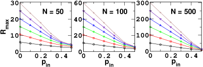
Figure 1: (Color online) Largest real part of eigenvalue, averaged over 2000 realizations of the network, as a function of probability of I couplings $p_{\mathrm{i}n}$ for various average degree $\langle k\rangle=10(\circ),20(\square),30(\diamondsuit),40(\nabla),50(\triangle)$ and $60(\star)$ from bottom to top. Left panel is for $N=50$, middle for $N=100$ and right panel for $N=500$.

After constructing an Erdös-Renýi random network net_review with network size $N$ and connection probability $p$ with a corresponding adjacency matrix ($A$) having entries 0 and 1, I connections are introduced with a probability $p_{\mathrm{i}n}$ as follows. A node is randomly selected as I with the probability $p_{\mathrm{i}n}$ and all connections arising from such nodes yield $-1$ entry into corresponding matrix $A$. For $p_{\mathrm{i}n}$ being $0$, which assimilates the correlation $A_{ij}A_{ji}=1$, network is undirected with $A$ being symmetric entailing all real eigenvalues. Maximum eigenvalue for this network scales as $R_{\mathrm{m}ax}\sim pN$ Ferenc , where quantity $pN$ is referred to as average degree $\langle k\rangle$ of the network. Upon introduction of directionality, complex eigenvalues start appearing in conjugate pairs, and for $p_{\mathrm{i}n}=0.5$, bulk of the eigenvalues is distributed in a circular region of radius $\sqrt{Np(1-p)}$ pre2011a . Note that for a random network with entries 1 and $-1$, the radius of circular bulk region scales with square root of the average degree of the network i.e. $\sqrt{pN}$, and all eigenvalues including the largest lie within the bulk.

III Transition from the normal to the GEV statistics

We investigate $R_{\mathrm{m}ax}$ of random networks as a function of $p_{\mathrm{i}n}$. Fig. 1 elucidates that, as directionality is introduced in terms of I couplings, the mean of $R_{\mathrm{m}ax}$ decreases linearly up to a certain threshold value, with subsequent decrease in a nonlinear fashion without any known functional form in terms of network parameters. For the linear regime $0\lesssim p_{\mathrm{i}n}\lesssim 0.4$, fitting with a straight line yields the following relation between $R_{\mathrm{m}ax}$ and $p_{\mathrm{i}n}$:

$$R_{\mathrm{m}ax}\sim pN-(2Np)p_{\mathrm{i}n}$$ (2)

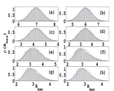
Figure 2: (Color online) Statistics of $R_{\mathrm{m}ax}$ at different values of I coupling probability $p_{\mathrm{i}n}$. The histograms are numerical results, solid and dashed lines correspond to the normal and the GEV fit respectively. For each case, size of the network is $N=100$ and connection probability $0.06$ which leads to the average degree $\langle k\rangle=6$. (a), (b), (c), (d), (e), (f), (g) and (h) correspond to $p_{\mathrm{i}n}$ being 0, 0.1, 0.3, 0.4, 0.42, 0.46, 0.48 and 0.50 respectively.

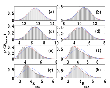
Figure 3: (Color online) $R_{\mathrm{m}ax}$ statistics for network parameters $N=100$ and $p=0.12$ entailing $\langle k\rangle=12$ average degree. (a), (b), (c), (d), (e), (f), (g) and (h) correspond to $p_{\mathrm{i}n}$ = 0.00, 0.10, 0.30, 0.40, 0.42, 0.46, 0.48 and 0.50 respectively. The histograms are numerical results, solid and dashed lines are obtained after fitting the data with the normal and the GEV distributions respectively.

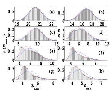
Figure 4: (Color online) For $N=100$ and $p=0.2$ which corresponds to $<k>=20$ average degree. Subfigures (a), (b), (c), (d), (e), (f), (g) and (h) correspond to $p_{\mathrm{i}n}$ being 0, 0.1, 0.3, 0.4, 0.42, 0.46, 0.48 and 0.5 respectively. The histograms represent numerical result, solid and dashed lines are obtained by fitting the date with the normal and the GEV distributions respectively.

Fig. 2 depicts statistics for largest real part of eigenvalue for $N=100$ and average degree $<k>=6$. The curve is fitted with the GEV distribution from Eq. 1 note1 . For $0\lesssim p_{\mathrm{i}n}\lesssim 0.4$, nature of distribution is normal, however, as reflected by the left panel of Fig. 1, the mean decreases in agreement to the equation Eq. 2. Variances of the data as well as of fitted curves increase with a faster rate for $0\lesssim p_{\mathrm{i}n}\lesssim 0.1$ after which there is a fall in its rate of increment. The variance achieves a peak at $p_{\mathrm{i}n}\sim 0.30$, and then decreases with a slower rate. The behavior of largest eigenvalue statistics is more complex in the range $0.40\lesssim p_{\mathrm{i}n}\lesssim 0.50$, where it can be modeled using extreme value statistics. Figs. 2(e)-(h) and negative values of the parameter $\xi$ indicate that statistics converge to the Weibull distribution. Calculations of shape parameter and detailed discussion on fitting has been exemplified in the section VIII.

As connection probability or $\langle k\rangle$ increases, this phenomena of transition from the normal to the GEV statistics for $R_{\mathrm{m}ax}$ becomes more prominent. Fig. 3, plotted for $N=100$ and $<k>=12$, repeats the normal distribution behavior for $p_{\mathrm{i}n}=0$, which corresponds to a symmetric random matrix with entries $0$ and $1$. Till $p_{\mathrm{i}n}\lesssim 0.3$, $R_{\mathrm{m}ax}$ statistics more or less conforms to the normal distribution. At $p_{\mathrm{i}n}=0.4$, the statistics deviates from the normal distribution, with fitting accuracy being higher for the GEV. With a further increase in the value of $p_{\mathrm{i}n}$, there is a transition to the GEV statistics as illustrated by Fig. 3 at $p_{\mathrm{i}n}\sim 0.46$. This behavior of the $R_{\mathrm{m}ax}$ continues thereafter.

As $\langle k\rangle$ increases further, $\rho(R_{\mathrm{m}ax})$ keeps emulating the normal distribution at $p_{\mathrm{i}n}=0$ and the GEV statistics at $p_{\mathrm{i}n}=0.5$. At intermediate $p_{\mathrm{i}n}$ values, it manifests different behaviors than demonstrated for lower connection probabilities as described by Figs. 2 and  3. As soon as $p_{\mathrm{i}n}$ increases from value $0$, the $R_{\mathrm{m}ax}$ statistics starts deviating from the normal distribution, and for intermediate $p_{\mathrm{i}n}$ values, for example at $p_{\mathrm{i}n}=0.2$ and $p_{\mathrm{i}n}=0.3$ in Fig. 4, it neither fits with the normal nor with the GEV statistics. As value of $p_{\mathrm{i}n}$ increases, $R_{\mathrm{m}ax}$ statistics indicates a closer fitting with the GEV, and more deviation from the normal at $p_{\mathrm{i}n}=0.4-0.42$ as implied from Fig. 4(d)-(e). Further increase in $p_{\mathrm{i}n}$ prompts a good fitting with the GEV statistics at $p_{\mathrm{i}n}=0.44$, and this good fitting persists thereafter. Detailed discussion on true GEV statistics is provided in the section VIII.

Aforementioned behavior indicates that smaller $\langle k\rangle$ values induce a smooth transition from the normal to the GEV statistics, and for almost all values of $p_{\mathrm{i}n}$ the largest eigenvalue statistics remains close to either one of them. Whereas larger $\langle k\rangle$ values construe a rich behavior of $\rho(R_{\mathrm{m}ax})$. It ensues the normal distribution till certain range of $p_{\mathrm{i}n}$ and after that manifests deviation from it displaying a rapid change in the statistics as $p_{\mathrm{i}n}$ is incremented. For this intermediate $p_{\mathrm{i}n}$ range $R_{\mathrm{m}ax}$ statistics deviates from the normal as well as the GEV substantially. As $p_{\mathrm{i}n}$ increases further, the statistics fits better for the GEV as compared to the normal, finally elucidating a legitimate fitting with the GEV distribution at $p_{\mathrm{i}n}$ being 0.5.

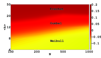
Figure 5: (Color online)Phase diagram in two parameters space $N$ and $\langle k\rangle$ elucidating nature of GEV statistics based on the value of shape parameter $\xi$, and tail of the distribution at $p_{\mathrm{i}n}=0.5$.

IV Transition from Weibull to Fréchet

At these $p_{\mathrm{i}n}$ values where statistic fits well with the GEV, the parameter $\xi$, in the tables of section VIII, reveals that indeed the distribution complies one of the three different statistics, viz. Gumbel, Weibull and Fréchet, depending upon $\langle k\rangle$. For small $\langle k\rangle$, corresponding to sparser networks, the GEV statistics espoused Weibull distribution, whereas with an increase in connection probability it indicates a transition to Fréchet distribution through Gumbel. Phase diagram Fig. 5 illustrates this behavior for various values of $N$ and $\langle k\rangle$. For a definite shape parameter range the Weibull and the normal states have a close resemblance, the statistics in the intermediate regions of $p_{\mathrm{i}n}$ consequently emulating to one of them. Whereas, Gumbel and Fréchet are much deviated from the normal, hence in the transition from the normal to the Gumbel or Fréchet, $\rho(R_{\mathrm{m}ax})$ may not abide by any of the statistics, and explains a scabrous behavior of $R_{\mathrm{m}ax}$ in the intermediate $p_{\mathrm{i}n}$ region.

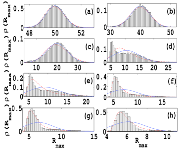
Figure 6: (Color online) Statistics of $R_{\mathrm{m}ax}$ at different values of I coupling probability $p_{\mathrm{i}n}$. The histograms are numerical results, solid and dashed lines correspond to normal and GEV fit respectively. For each case, size of the network is $N=100$ and connection probability $0.5$ leading to average degree $\langle k\rangle=50$. (a), (b), (c), (d), (e), (f), (g) and (h) correspond to $p_{\mathrm{i}n}$ being 0, 0.1, 0.3, 0.4, 0.42, 0.46, 0.48 and 0.50 respectively.

For the larger $\langle k\rangle$ values, $R_{\mathrm{m}ax}$ does not apprise GEV statistics even at $p_{\mathrm{i}n}=0.5$, Fig. 6 and the value of $\xi$ reflect a Fréchet behavior although KS test rejects it. In order to understand such an impact of denseness on $R_{\mathrm{m}ax}$ behavior, we investigate tail behavior of the parent distribution, and Fig. 7(c) reveals that it is deviated from a power-law behavior for larger $R_{\mathrm{m}ax}$ values, manifesting a deviation from GEV distribution, whereas tail behaviors corresponding to $\langle k\rangle$= 12 and $\langle k\rangle$= 20 imitates exponential and power law decay, respectively as indicated by Fig. 7 (a) and (b), reinforcing Gumbel and Fréchet distribution respectively for their maxima. Higher $\langle k\rangle\gtrsim 20$ values for which spectra do not exhibit GEV even for $p_{\mathrm{i}n}=0.5$, may be ascribed to the correlation in spectra arising from $1$ and $-1$ entries competing with each other. Fig. 7 indicates existence of two different scales for $\langle k\rangle=50$, providing a plausible explanation of deviation from GEV.

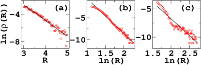
Figure 7: (Color online)Tail behavior of probability density function for real part of eigenvalues for network size $N=100$ and $p_{\mathrm{i}n}=0.5$. Circles represent data points, and solid line represents fitting with a straight line. Figures are plotted for three different average degrees (a) $\langle k\rangle=12$, (b) $\langle k\rangle=20$ and (c) $\langle k\rangle=50$.

Furthermore, revelation of the transition from Weibull to Fréchet as a function of connection probability or average degree $\langle k\rangle$ of the network, adds networks to the list of wide physical systems exhibiting this transition. For example, extreme intensity statistics in relation to complex random states manifest the Weibull distribution in case of minimum intensity and the Gumbel distribution for maximum intensity Arul_prl2008 . For mass transport models distribution of largest mass displays the Weibull, Gumbel and Fréchet distribution depending upon critical density. Majumdar2008_JStatMech . For non-interacting Bosons, level density follows one of these three distributions depending upon characteristic exponent of growth of underlying single particle spectrum gev_boson .

The interpretation of our result of transition from Weibull to Fréchet in terms of the stability of underlying systems can be drawn as follows. For large number of I nodes present in the network, the statistics of $R_{\mathrm{m}ax}$ for denser networks are more right skewed and more deviated from a normal distribution as compared to the sparser networks, which indicates that higher values of $R_{\mathrm{m}ax}$ are more probable for denser networks. This transpires that the probability with which a network ushers to an unstable system is more for denser networks than for the sparser ones. Robert May, in his landmark paper MayNature1972 , concluded that a randomly assembled web becomes less robust (measured in terms of its dynamical stability) as its connectivity increases. Our results supports this interpretation for the networks having I and E couplings, which is not only based on the average mean behavior of largest eigenvalue but also based on its distribution modeled using the GEV statistics.

V Impact of I-I/E-E and I-E/E-I couplings

Our model elucidates a profound impact of I-E ratio on both the mean and statistics of $R_{\mathrm{m}ax}$, hence indicating a probable impact on the stability or dynamical properties of corresponding system. To get insight into the transition from one statistics to another, first we discuss the importance of I-E couplings, followed by an analysis based on a measure capturing I-E couplings ratio. There exists plenty of behaviors and processes exhibited by neural systems which have been attributed to the ratio or balance between E and I inputs Science1996_in_ex ; hippo . In cortex, inter-neurons responsible for inhibition play an important function in regulating activity of principal cells. When inhibition is blocked pharmacologically, cortical activity becomes epileptic Dichter1987_Science , and neurons may lose their selectivity to different stimulus Sillito1975 . These and other data indicate that an interplay between excitation and inhibition portrays a substantial role in determining the cortical computation PNAS2004_in_ex .

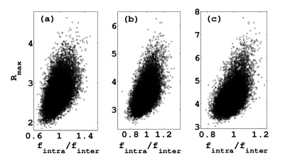
Figure 8: Plots of $R_{\mathrm{m}ax}$ against $f_{\mathrm{i}ntra}/f_{\mathrm{i}nter}$ for different values of average degree at $p_{\mathrm{i}n}=0.5$ with network size $N=100$ and sample size 20000. Panels (a), (b) and (c) corresponds to k = 6, 12 and 20 respectively.

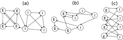
Figure 9: Schematic diagram illustrating (a) a modular-type structure, (c) a bipartite type structure, and (b) the intermediate of these two extremes. Dots and arrows represent inhibitory and excitatory links, respectively.

In order to understand the origin of two different statistics at $p_{\mathrm{i}n}$ $0$ and $0.5$, we define a measure $f_{\mathrm{i}ntra}/f_{\mathrm{i}nter}$ which captures an competition between I-I and E-E couplings with I-E couplings. The quantities $f_{\mathrm{i}nter}$ and $f_{\mathrm{i}ntra}$ correspond to fraction of (I-E) and (I-I) + (E-E) couplings respectively. Fig. 8 plots $R_{\mathrm{m}ax}$ against $f_{\mathrm{i}ntra}/f_{\mathrm{i}nter}$ exhibiting a positive correlation between the two. Presence of few scattered dots towards the rightmost top corner of the Fig. 8(a) for $\langle k\rangle=6$ clearly reveals that underlying network has maximum -intra connections owing to high $f_{\mathrm{i}ntra}/f_{\mathrm{i}nter}$ and $R_{\mathrm{m}ax}$. These figures indicate that the connections between neurons akin escort to more of an unstable system as compared to a balanced structure Rajan . Moreover, in realistic neuronal network, connectivity is sparser between excitatory neurons than between other pairs excit-inhibit , which correspond to the region lying towards the left of the Fig. 8 suggesting that networks with less intra-connections are more stable. The measure $f_{\mathrm{i}ntra}/f_{\mathrm{i}nter}$ is bounded between two extreme structures: modular (all I-I and/or E-E connections) and bipartite (all E-I or I-E connections) (Fig. 9).

Various realizations of the considered model may induce networks having (i) modular type structure (Fig. 9a), (ii) bipartite type of structure (Fig. 9c) and (iii) intermediate structure lying in between these two (Fig. 9b). Note that network structure remains same in all three cases, it is only the type of node (I or E) at two ends of a connection which decides the configurations mentioned above. An ideal bipartite structure would bring upon an anti-symmetric matrix consequently having all imaginary eigenvalues. Though networks considered here do not consort to an ideal bipartite arrangement as depicted in Fig. 9(c), for high values of $f_{\mathrm{i}nter}$ as elucidated in the Fig. 8, it is expected to lie close to this arrangement which explains the origin of lower $R_{\mathrm{m}ax}$ to the left of Fig. 8. What follows is that larger I-E couplings drives to lower values of $R_{\mathrm{m}ax}$, which may be even $0$ for an ideal case of bipartite structural arrangement entailing a complete anti-symmetric matrix, whereas larger I-I or E-E couplings, which may be considered as modular type arrangement direct to higher $R_{\mathrm{m}ax}$ values which may sometimes be unusually very large for certain network configurations, probably being one of the plausible reasons behind the origin of GEV statistics. Furthermore, the discussion elaborating Fig. 8 apparently sheds light on the origin of stability of network configurations having more inter-connections, in turn supporting bipartite type topology over a modular one as proposed in Lazar for real world network.

VI Conclusion and Implications

To conclude, we have analyzed $R_{\mathrm{m}ax}$ statistics of networks having I and E couplings. A linear decrease, followed by a non-linear one, in $R_{\mathrm{m}ax}$ as a function of $p_{\mathrm{i}n}$ indicates that an increase in complexity, in terms of inclusion of I nodes, increases the stability of underlying system. For the range where $R_{\mathrm{m}ax}$ mean ensues the linear dependence on $p_{\mathrm{i}n}$, the statistics mostly yields a normal distribution, and after this critical $p_{\mathrm{i}n}$ value there is a transition to the GEV statistics. The versatile situation arising from I-I, I-E competition, bringing upon GEV statistics, has not been observed for zero $p_{\mathrm{i}n}$ value, and hence may be attributed to the rich behavior of $R_{\mathrm{m}ax}$ in the presence of I nodes.

Though modeling real brain networks needs to account for more properties such as specific degree distribution, hierarchical structure etc, which may bring upon a richer largest eigenvalue pattern under_prep , an impact of I nodes impels a drastic change in its spectral properties illustrating extreme events which has been envisaged upon in this paper. Asymmetric matrices considered here, motivated by brain networks, elucidate a different statistical property of $R_{\mathrm{m}ax}$ than that of non-Hermitian matrices motivated by ecological webs ginibre . Moreover, the universal GEV distribution displayed by largest eigenvalue of networks propagates theory of extreme value statistics, which suggests that a model which fits with all eigenvalues or describe fluctuations of all eigenvalues SJ_pre2007b may not be a good model for the largest one.

Recent years have seen a fast development in merging of extreme statistics tools and random matrix theory. The present work extends this general perspective to complex networks. To our knowledge, this is the first work on networks demonstrating that the largest eigenvalue of a network, at particular I-E coupling ratio, can be modeled by the GEV statistics. The transition of the statistics from one type to another as a function of I connections has crucial implications in predicting and analyzing network functions and behaviors in extreme situations rev_syn .

VII Acknowledgment

SKD acknowledges UGC for financial support. SJ thanks DST for funding. It is a pleasure to acknowledge Dr. Changsong Zhou (Hongkong Baptist University) for useful discussions on brain networks at several occasions, and Dr. A. Lakshminarayan (IITM) for suggestions on GEV statistics.

VIII Appendix

We use Kolmogorov-Smirnov (KS) test to characterize hypothesized model of our data. The KS test is known to be superior to other techniques such as chi-square test Massey for identifying a particular distribution. For example, in the context of networks, the said test has been performed to confirm power law for a given network data Clauset . The function kstest of MATLAB Statistics Toolbox is used to verify the acceptance of a given statistics at $95\%$ level of confidence if its corresponding p-value of KS test is greater than 0.05.

In some of the parameter regimes, GEV distribution resembles the normal distribution owing to its shape parameter $\xi$, which characterizes it as Weibull distribution Dubey , and a particular distribution is confirmed using KS test. Another example demonstrating the quality of our results can be exemplified with larger $\langle k\rangle$ values, where for $p_{\mathrm{i}n}>0.46$, though distribution looks more like Fréchet (Fig.4(d)), KS test accepts Fréchet distribution at $p_{\mathrm{i}n}=0.5$ only. We perform KS test for sample size 5000, which is large enough to approve a statistics. For example, Sanjib accounts for 4000 sample size for performing KS test, and in Plerou , it is implemented to affirm GOE and GSE statistics for random matrices with sample size 1000.

It might be possible that for some network parameters, KS test accepts normal as well as Weibull distributions, as depicted earlier by the fact that GEV distribution in a certain shape parameter range resembles normal distribution Dubey . To address this issue, we increase the sample size from 5000 to 20000 for which KS test accepts either normal or Weibull distribution. For example at $\langle k\rangle=6$ for various $p_{\mathrm{i}n}$ values 0.0, 0.3, 0.4, the sample size is increased to 20000 where only one distribution is accepted by the KS test. Similarly for $\langle k\rangle=12$ and $p_{\mathrm{i}n}=0.1$ and $0.3$, the sample size is increased to 20000 for implementation of KS test.

Table 1: Estimated parameters of GEV and normal distributions for $R_{\mathrm{m}ax}$ for different inhibitory coupling probability ($p_{\mathrm{i}n}$). For each case, size of network is $N=100$ and average degree $\langle k\rangle$ = 6. Sample size is 5000 for all $p_{\mathrm{i}n}$ values except for $\star$ entries for which sample size is 20000.

$p_{\mathrm{i}n}$	$\xi$ of GEV	$\sigma$ of GEV	$\mu$ of GEV	p-value of KS test for GEV	$\mu$ of Normal	$\sigma$ of Normal	p-value of KS test for Normal
0.00*	-0.2392	0.3509	6.8484	0.0013	6.9813	0.3548	0.3717
0.10	-0.2204	0.4806	5.8032	0.0003	5.9893	0.4800	0.4127
0.30*	-0.2248	0.5410	4.0107	0	4.2210	0.5505	0.2966
0.40	-0.1945	0.5230	3.2444	0.0062	3.4606	0.5501	0.0000
0.42*	-0.1695	0.4960	3.0695	0.0637	3.2852	0.5355	0.0000
0.46	-0.0933	0.4178	2.8485	0.3270	3.0558	0.4832	0.0000
0.48	-0.0881	0.3767	2.7845	0.3983	2.9725	0.4374	0.0000
0.50	-0.1104	0.3492	2.7593	0.9919	2.9261	0.3955	0.0000

Table 2: Estimated parameters of GEV and normal distributions for $R_{\mathrm{m}ax}$ for different inhibitory coupling probability ($p_{\mathrm{i}n}$). For each case, size of network is N = 100 and average degree $\langle k\rangle$ = 12.

$p_{\mathrm{i}n}$	$\xi$ of GEV	$\sigma$ of GEV	$\mu$ of GEV	p-value of KS test for GEV	$\mu$ of Normal	$\sigma$ of Normal	p-value of KS test for Normal
0.00	-0.2482	0.4693	12.611	0.0262	12.7853	0.4702	0.6673
0.10*	-0.3009	0.8671	10.272	0	10.5660	0.8475	0.0001
0.30*	-0.2370	1.0494	6.1683	0.0187	6.5675	1.0617	0.4473
0.40	-0.1742	0.9214	4.4642	0.0136	4.8629	0.9946	0.0001
0.42	-0.1135	0.8319	4.1918	0	4.5937	0.9456	0.0000
0.46	0.0584	0.5809	3.7219	0.0001	4.0940	0.7793	0.0000
0.48	0.0711	0.4908	3.5951	0.0709	3.9159	0.6771	0.0000
0.50	0.0232	0.4500	3.5744	0.7076	3.8454	0.5916	0.0000

Table 3: Estimated parameters of GEV and normal distributions for $R_{\mathrm{m}ax}$ for different inhibitory coupling probability ($p_{\mathrm{i}n}$). For each case, size of network is N = 100 and average degree $\langle k\rangle$ = 20.

$p_{\mathrm{i}n}$	$\xi$ of GEV	$\sigma$ of GEV	$\mu$ of GEV	p-value of KS test for GEV	$\mu$ of Normal	$\sigma$ of Normal	p-value of KS test for Normal
0.00	-0.2293	0.5546	20.388	0.0443	20.601	0.5587	0.9446
0.10	-0.2999	1.3779	16.325	0.0025	16.790	1.3371	0.0183
0.30	-0.2420	1.8081	8.7824	0.0037	9.4622	1.8091	0.2053
0.40	-0.1231	1.4617	5.7608	0	6.4558	1.6475	0.0000
0.42	-0.0221	1.2347	5.2248	0	5.9203	1.5168	0.0000
0.46	0.1984	0.7740	4.5096	0	5.1254	1.2005	0.0000
0.48	0.1836	0.6413	4.3695	0.0035	4.8724	1.0147	0.0000
0.50	0.1133	0.5494	4.3218	0.1123	4.7080	0.8266	0.0000

Table 4: Estimated parameters of GEV and normal distributions for $R_{\mathrm{m}ax}$ for different inhibitory coupling probability ($p_{\mathrm{i}n}$). For each case, size of network is N = 100 and average degree $\langle k\rangle$ = 50. Since for none of the $p_{\mathrm{i}n}$ values data fits with the GEV distribution, sample size here is increased from 5000 to 20000 for all $p_{\mathrm{i}n}$ values to inquire if higher sample size confirms a GEV distribution.

$p_{\mathrm{i}n}$	$\xi$ of GEV	$\sigma$ of GEV	$\mu$ of GEV	p-value of KS test for GEV	$\mu$ of Normal	$\sigma$ of Normal	p-value of KS test for Normal
0.00	-0.2354	0.7033	49.714	0.0000	49.982	0.7073	0.9484
0.10	-0.2787	3.2684	38.806	0.0000	39.955	3.1831	0.0000
0.20	-0.2803	4.2905	28.419	0.0000	29.920	4.1866	0.0004
0.30	-0.2304	5.0941	17.956	0.0000	19.897	5.0239	0.0000
0.40	0.0676	3.4118	8.2755	0.0000	10.489	4.4492	0.0000
0.42	0.4561	2.2051	6.6802	0.0000	9.0732	3.9636	0.0000
0.44	0.5707	1.5312	5.9710	0.0000	7.9807	3.3925	0.0000
0.46	0.5063	1.1223	5.6447	0.0000	7.1094	2.7603	0.0000
0.48	0.3859	0.8741	5.4775	0.0000	6.4787	2.1008	0.0000
0.50	0.24152	0.7562	5.4673	0.0000	6.1574	1.5986	0.0000

For $\langle k\rangle$ values ranging between 16 and 20, the distribution lies close to Fréchet but not exactly Fréchet even for 20000 sample size, thus rendering KS test to reject it. This is supposedly the bottleneck of increasing sample size. We perform KS test for even a higher sample size (50000), and it does not accept the Fréchet distribution (even though distribution keeps lying close to the Fréchet), hence demonstrating fairness of our data and the technique adopted to conclude a particular distribution.
We have also observed an effect of network size on the value of shape parameter $\xi$. For example $\langle k\rangle=6$, networks size $N=100$ and $N=1000$ yield a $\xi$ which characterizes Weibull distribution, whereas for $\langle k\rangle=20$, size $N=100$ reflects Fréchet, and size $N=1000$ reflects Gumbel distribution. The phase diagram presented in Fig. 5 corresponds to $p_{\mathrm{i}n}=0.5$, for which we get GEV statistics till certain $\langle k\rangle$ values. For the larger $\langle k\rangle$ values when $R_{\mathrm{m}ax}$ does not comply with GEV statistics even at $p_{\mathrm{i}n}=0.5$, Fig. 6 and the value of $\xi$ in the Table.4 suggest a Fréchet behavior however KS test rejects it.

References

- (1) P. Van Meighem, J. Omic, and R. E. Kooij, IEEE/ACM Trans. Netw. 17, 1 (2009).
- (2) J. G. Restrepo, E. Ott and B. R. Hunt, Phys. Rev. E 71, 036151 (2005).
- (3) H. Sompolinsky, A. Crisanti and H. J. Sommers, Phys. Rev. Lett. 61, 259 (1988).
- (4) B. Cessac and J. A. Sepulchre, Chaos 16, 013104 (2006).
- (5) T. P. Vogels, K. Rajan and L. F. Abbott, Annu. Rev. Neurosci. 28, 357 (2005).
- (6) K. Rajan and L. F. Abbott, Phys. Rev. Lett. 97, 188104 (2006).
- (7) A. V. Goltsev et. al., Phys. Rev. Lett. 109 128702 (2012).
- (8) R. M. May, Nature 238 413 (1972).
- (9) J. Quirk and R. Ruppert, Rev. Econ. Stud. 32(4), 311 (1965).
- (10) C. A. Tracy and H. Widom, Proceedings of the International Congress of Mathematicians (Higher Education Press, Beijing, 2002), Vol. 1, pp. 587-596.
- (11) E. J. Gumbel, Statistics of Extremes (Columbia University Press, 1958).
- (12) A. Lakshminarayan et. al., Phys. Rev. Lett. 100, 044103 (2008).
- (13) T. Antalabin et. al., EPL 88 59001 (2009) .
- (14) R. Labbé and G. Bustamante, arXiv:1201.4802
- (15) T. Antal et. al., Phys. Rev. Lett. 87 240601 (2001).
- (16) S. Joubaud et. al., Phys. Rev. Lett. 100 180601 (2008).
- (17) B. P. Van Milligen et. al., Phys. Plasmas, 12 (2005) 052507.
- (18) V. L. Girko, Theory Probab. Appl. 29, 694 (1984).
- (19) B. J. Rider, Phys. A Mat. Gen. 36, 3401 (2003).
- (20) P. V. Mieghem Graph Spectra, (Cambridge Univ. Press 2012).
- (21) D. H. Kim and A. E. Motter, Phys. Rev. Lett. 98, 248701 (2007).
- (22) Z. Füredi and J. Komlós, Combinatorica 1, 233 (1981).
- (23) M. Krivelevich and B. Sudakov, Combinatorics, Probab. Comput. 12, 61 (2003).
- (24) R. Gray and P. Robinson, Neurocomputing 70, 1000 (2007).
- (25) O. Sporns Networks of the Brain (The MIT Press Cambridge 2011) (
- (26) R. Albert and A.-L. Barabási, Rev. Mod. Phys. 74 47 (2002).
- (27) F. Juhasz, Discrete Math. 41, 161 (1982).
- (28) S. Jalan, G. M. Zhu and B. Li, Phys. Rev. E 84, 046107 (2011).
- (29) For numerical analysis, functions in MATLAB statistics toolbox such as gevfit and gevpdf have been used. These functions compute maximum likelihood estimation for parameters of GEV with confidence level. One of the earlier usage of this package includes numerical study of extreme value distribution in a discrete dynamical system with block maxima approach, where gevfit and gcdf functions have been used for robust estimation of its parameters Davide. In this reference unnormalized data is directly fitted with GEV and relation between normalized sequences as well as parameters of GEV have been established.
- (30) M. Evans and S. Majumdar, J. Stat. Mech.:Th. and Exp. P05004 (2008).
- (31) A. Comtet, P. Leboeuf and S. N. Majumdar, Phys. Rev. Lett. 98, 070404 (2007).
- (32) C. van Vreeswijk and H. Sompolinsky, Science 274, 1724 (1996).
- (33) I. Fried et. al., Cereb Cortex 12, 575 (2002).
- (34) M. A. Ditcher and G. F. Ayala, Science 10 4811 (1987).
- (35) A. M. Sillito, J. Physiol 250 305 (1975).
- (36) O. Prange et. al., Proc. Natl. Acad. Sci. USA 101 13915 (2004).
- (37) N. M. Economo and J. A. White, PLoS Comput Biol 8, 1 (2012).
- (38) A. Lazar, G. Pipa and J. Triesch, Front Comput Neurosci 3 23 (2009).
- (39) S. Jalan et. al. (unpublished)
- (40) P. Forrester and T. Nagao, Phys. Rev. Lett. 99 050603 (2007).
- (41) S. Jalan and J. N. Bandyopadhyay, Phys. Rev. E 76 046107 (2007).
- (42) A. Arenas et. al., Physics Reports 469 93 (2008).
- (43) J. Massey and J. Franck, J. Am. Stat. Assoc. 46 68 (1951).
- (44) A. Clauset, C. R. Shalizi and M. E. J. Newman, SIAM Rev. 5 1, 661 (2009).
- (45) S. D. Dubey, Nav. Logist. Res. Q. 14 69 (1967).
- (46) S. Sabhapandit and S. N. Majumdar, Phys. Rev. Lett. 98 140201 (2007).
- (47) V. Plerou, P. Gopikrishnan, B. Rosenow, L. A. N. Amaral and H. E. Stanley, Phys. Rev. Lett. 83, 1471 (1999).