Supervised Heterogeneous Multiview Learning for Joint Association Study and Disease Diagnosis

Abstract

Given genetic variations and various phenotypical traits, such as Magnetic Resonance Imaging (MRI) features, we consider two important and related tasks in biomedical research: i)to select genetic and phenotypical markers for disease diagnosis and ii) to identify associations between genetic and phenotypical data. These two tasks are tightly coupled because underlying associations between genetic variations and phenotypical features contain the biological basis for a disease. While a variety of sparse models have been applied for disease diagnosis and canonical correlation analysis and its extensions have bee widely used in association studies (e.g., eQTL analysis), these two tasks have been treated separately. To unify these two tasks, we present a new sparse Bayesian approach for joint association study and disease diagnosis. In this approach, common latent features are extracted from different data sources based on sparse projection matrices and used to predict multiple disease severity levels based on Gaussian process ordinal regression; in return, the disease status is used to guide the discovery of relationships between the data sources. The sparse projection matrices not only reveal interactions between data sources but also select groups of biomarkers related to the disease. To learn the model from data, we develop an efficient variational expectation maximization algorithm. Simulation results demonstrate that our approach achieves higher accuracy in both predicting ordinal labels and discovering associations between data sources than alternative methods. We apply our approach to an imaging genetics dataset for the study of Alzheimer’s Disease (AD). Our method identifies biologically meaningful relationships between genetic variations, MRI features, and AD status, and achieves significantly higher accuracy for predicting ordinal AD stages than the competing methods.

1 Introduction

Recent advances in biomedical research have provided new opportunities to study diseases – for example, Alzheimer’s disease (AD), the most common neurodegenerative disorder – from multiple data sources. For example, one data source contains genetic variations, such as single nucleotide polymorphisms (SNPs), which can help us understand the genetic basis of diseases. Another data source can be molecular and clinical phenotypes, such as Magnetic Resonance Imaging (MRI) data, which can reveal important phenotypic changes in patients.Finding associations between different data sources can reveal unknown biological relationships and has a wide range of applications in computational biology [1], epidemiology [2], computational neural science [3], and imaging genetics [4]. In addition to the genotypes and phenotypic traits, we have valuable labeled information about disease stages from patient medical records. Thus we face a new data analysis setting where the objective is two-fold: i) finding associations between different data sources and ii) selecting relevant (groups of) features from all the sources to predict ordinal disease stages.

Many statistical approaches have been developed to discover associations or select features (or variables) for prediction in a high dimensional problem. For association studies, representative approaches are canonical correlation analysis (CCA) and its extensions [5, 6]. These approaches treat different data sources as separate linear projections from a common latent representation. These approaches have been widely used in expression quantitative trait locus (eQTL) analysis. For example, Parkhomenko et al. [7] applied sparse CCA (sCCA) to find relationships between genetic loci and gene expression levels in Utah families; Witten and Tibshirani [8] used sCCA to reveal associations between gene expression and DNA copy variation; and Chen et al. [9] used structured CCA for pathway selection. For disease diagnosis based on high dimensional biomarkers, popular approaches include lasso [10], elastic net [11], and group lasso [12], and Bayesian automatic relevance determination [13, 14]. Here we treat genotypes or phenotypes as predictors (i.e., biomarkers) and the disease status as the response in a linear regression or classification setting. Non-zero estimated regression or classification weights indicate relevant biomarkers for the disease [15, 16].

Despite their wide success in many applications, these approaches are limited by the following factors:

• Most association studies neglect the supervision from the disease status. Because many diseases, such as AD, are a direct result of genetic variations and often highly correlated to clinical traits, the disease status provides useful yet currently unutilized information for finding relationships between genetic variations and clinical traits.

• For disease diagnosis, most sparse approaches use classification models and do not consider the order of disease severity. For subjects in AD studies, there is a natural severity order from being normal to mild cognitive impairment (MCI) and then from MCI to AD. Classification models cannot capture the order in AD’s severity levels. Furthermore, the classification approaches are often based on conditional models (e.g., logistic regression) and ignore relationships between multiple views.

• Most previous methods are not designed to handle heterogeneous data types. The SNPs values are discrete (and ordinal based on an additive genetic model), while the imaging features are continuous. Popular CCA or lasso-type methods simply treat both of them as continuous data and overlook the heterogeneous nature of the data.

To address these problems, we propose a new Bayesian approach that unifies multiview learning with sparse ordinal regression for joint association study and disease diagnosis. In the new approach, genetic variations and phenotypical traits are generated from common latent features based on separate sparse projection matrices and suitable link functions and the common latent features are used to predict the disease status based on Gaussian process ordinal regression (See Section 2). To enforce sparsity in projection matrices, we assign spike and slab priors [17] over them; these priors have been shown to be more effective than $l_{1}$ penalty to learn sparse projection matrices [18, 19]. The sparse projection matrices not only reveal critical interactions between the different data sources but also identify groups of biomarkers in data relevant to disease status. Finding groups of biomarkers can avoid over-sparsification (i.e., selecting one instead of multiple correlated features), thus boosting the accuracy for disease diagnosis. It can also help provide a better biological understanding because these groups may form biologically units (i.e., pathways). Meanwhile, via its direct connection to the latent features, the disease status influences the estimation of the projection matrices so that it can guide the discovery of associations between heterogeneous data sources relevant to the disease. Hence we name this new method Supervised Heterogeneous Multiview Learning (SHML).

To learn the model from data, we develop a variational Bayesian expectation maximization (VB-EM) approach (See Section 3). It iteratively minimizes the Kullback Leibler divergence between a tractable approximation and exact Bayesian posterior distributions and provides an estimate to the model marginal likelihood. Maximizing this estimate enables us to automatically choose a suitable dimension for the latent features in a principled Bayesian framework.

In Section 4, we test our approach SHML on both synthetic and real datasets. On synthetic data, SHML achieves both higher estimation accuracy in recovering true associations between different views than CCA and sparse CCA, and higher prediction accuracy than multiple advanced alternative methods, such as the combination of CCA and elastic net, and Gaussian process ordinal regression [20]. We then apply SHML to an AD study. AD accounts for 60-80% of age-related dementia cases – one in eight older Americans has AD – and there is no cure for AD till now. It is believed that its underlying pathology precedes the onset of cognitive symptoms for many years [21]. Although AD studies have attracted a lot of attention from both academia and industry [22, 23], to our best knowledge, our paper presents the first (supervised) study to uncover associations between genotypes and phenotypic traits relevant to AD. Our results on Alzheimer’s Disease Neuroimaging Initiative (ADNI) data show that SHML achieves highest prediction accuracy among all the competing methods. Furthermore, SHML finds biologically meaningful predictive relationships between SNPs, MRI features, and AD status.

2 Model

First, let us describe the data. We assume there are two heterogeneous data sources: one contains continuous data – for example, MRI features – and one discrete ordinal data – for instance, SNPs. Note that we can easily generalize our model below to handle more views and other data types by adopting suitable link functions (e.g., a Possion model for count data). Given data from $n$ subjects, $p$ continuous features and $q$ discrete features, we denote the continuous data by a $p\times n$ matrix ${\bf X}=[{\bf x}_{1},\ldots,{\bf x}_{n}]$, the discrete ordinal data by a $q\times n$ matrix ${\bf Z}=[{\bf z}_{1},\ldots,{\bf z}_{n}]$, and the labels (i.e., the disease status) by a $n\times 1$ vector ${\bf y}=[y_{1},\ldots,y_{n}]^{\top}$. For the AD study, we let $y_{i}=0,1,\textrm{ and }2$ if the $i$-th subject is in the normal, MCI or AD condition, respectively.

To link two data sources ${\bf X}$ and ${\bf Z}$ together, we introduce common latent features ${\bf U}=[{\bf u}_{1},\ldots,{\bf u}_{n}]$ and assume ${\bf X}$ and ${\bf Z}$ are generated from ${\bf U}$ by sparse projection. The common latent feature assumption is sensible for association studies because both SNPs and MRI features are biological measurements of the same subjects. Note that ${\bf u}_{i}$ is the latent feature for the $i$-th subject and its dimension $k$ is estimated by evidence maximization. In a Bayesian framework, we give a Gaussian prior over ${\bf U}$, $p({\bf U})=\prod_{i}\mathcal{N}({\bf u}_{i}|{\bf 0},{\bf I})$, and specify the rest of the model (see Figure 1) as follows:

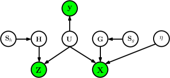
Figure 1: The graphical model of Supervised Heterogeneous Multiview Learning, where ${\bf X}$ is the continuous view, ${\bf Z}$ is the ordinal view, and ${\bf y}$ are the labels.

• Continuous data. Given ${\bf U}$, ${\bf X}$ is generated from

  $$p({\bf X}|{\bf U},{\bf G},\eta)=\prod_{i=1}^{n}\mathcal{N}({\bf x}_{i}|{\bf G}{\bf u}_{i},\eta^{-1}{\bf I})$$

  where ${\bf G}=[{\bf g}_{1},{\bf g}_{2},...{\bf g}_{p}]^{\top}$ is a $p\times k$ projection matrix, ${\bf I}$ is an identity matrix, and $\eta^{-1}{\bf I}$ is the precision matrix of the Gaussian distribution. We assign a Gamma prior over $\eta$, $p(\eta|r_{1},r_{2})=\textrm{Gamma}(\eta|r_{1},r_{2})$ where $r_{1}$ and $r_{2}$ are the hyperparameters and set to be $10^{-3}$ in our experiments.

• Ordinal data. For an ordinal observation $z\in\{0,1,\ldots,$
  $R-1\}$ its value is decided by which region an auxiliary variable $c$ falls in

  $$-\infty=b_{0}<b_{1}<\ldots<b_{R}=\infty.$$

  If $c$ falls in $[b_{r},b_{r+1})$, $z$ is set to be $r$. For the AD study, the SNPs ${\bf Z}$ takes values in $\{0,1,2\}$ and therefore $R=3$. Given a $q\times k$ projection matrix ${\bf H}=[{\bf h}_{1},{\bf h}_{2},...{\bf h}_{q}]^{\top}$, the auxiliary variables ${\bf C}=\{c_{ij}\}$ and the ordinal data ${\bf Z}$ are generated from

  $$p({\bf Z},{\bf C}|{\bf U},{\bf H}) =\prod_{i=1}^{q}\prod_{j=1}^{n}p(c_{ij}|{\bf h}_{i},{\bf u}_{j})p(z_{ij}|c_{ij})$$

  where

  $$p(c_{ij}|{\bf h}_{i},{\bf u}_{j}) =\mathcal{N}(c_{ij}|{\bf h}_{i}^{\top}{\bf u}_{j},1)$$

  $$p(z_{ij}|c_{ij}) =\sum_{r=0}^{2}\delta(z_{ij}=r)\delta(b_{r}\leq c_{ij}<b_{r+1}),$$

  where $\delta(a)=1$ if $a$ is true and $\delta(a)=0$ otherwise.

• Labels. The disease statuses ${\bf y}$ are ordinal variables too. To generate ${\bf y}$, we use a Gaussian process ordinal regression model [20] based the latent representation ${\bf U}$,

  $$p({\bf y}|{\bf U})=p({\bf y}|{\bf f})p({\bf f}|{\bf U}),$$

  where

  $$p({\bf f}|{\bf U}) =\mathcal{N}({\bf f}|{\bf 0},{\bf K}),$$

  $$p({\bf y}|{\bf f}) =\sum_{r=0}^{2}\delta(y_{i}=r)\delta(b_{r}\leq f_{i}<b_{r+1}),$$

  where $K_{ij}=k({\bf u}_{i},{\bf u}_{j})$ is the cross-covariance between ${\bf u}_{i}$ and ${\bf u}_{j}$. We can choose $k$ from a rich family of kernel functions such as linear, polynomial, and Gaussian kernels to model relationships between the labels ${\bf y}$ and the latent features ${\bf U}$.

  Note that the labels ${\bf y}$ are linked to the data ${\bf X}$ and ${\bf Z}$ via the latent features ${\bf U}$ and the projection matrices ${\bf H}$ and ${\bf G}$. Due to the sparsity in ${\bf H}$ and ${\bf G}$, essentially only a few groups of variables in ${\bf X}$ and ${\bf Z}$ are selected to predict ${\bf y}$. Note that each of group is linked to a feature in ${\bf U}$.

• Sparse Priors. Because we want to identify a few critical interactions between different data sources, we use spike and slab prior distributions [17] to sparsify the projection matrices ${\bf G}$ and ${\bf H}$. Specifically, we use a $p\times k$ matrix ${\bf S}_{g}$ to represent the selection of elements in ${\bf G}$: if $s_{ij}=1$, $g_{ij}$ is selected and follows a Gaussian prior distribution with variance $\sigma^{2}_{1}$; if $s_{ij}=0$, $g_{ij}$ is not selected and forced to almost zero (i.e., sampled from a Gaussian with a very small variance $\sigma^{2}_{2}$). Specifically, we have the following prior over ${\bf G}$:

  $$p({\bf G}|{\bf S}_{g},\boldsymbol{\Pi}_{g})=\prod_{i=1}^{p}\prod_{j=1}^{k}p(g_{ij}|s_{g}^{ij})p(s_{g}^{ij}|\pi_{g}^{ij})$$

  where

  $$p(g_{ij}|s_{g}^{ij}) =s_{g}^{ij}\mathcal{N}(g_{ij}|0,\sigma^{2}_{1})+(1-s_{g}^{ij})\mathcal{N}(g_{ij}|0,\sigma^{2}_{2}),$$

  $$p(s_{g}^{ij}|\pi_{g}^{ij}) ={\pi_{g}^{ij}}^{s_{g}^{ij}}(1-\pi_{g}^{ij})^{1-s_{g}^{ij}},$$

  where $\pi_{g}^{ij}$ in $\boldsymbol{\Pi}_{g}$ is the probability of $s_{g}^{ij}=1$, and $\sigma^{2}_{1}\gg\sigma^{2}_{2}$ (in our experiment, we set $\sigma^{2}_{1}=1$ and $\sigma^{2}_{2}=1o^{-6}$). To reflect our uncertainty about $\boldsymbol{\Pi}_{g}$, we assign a Beta hyperprior distribution:

  $$p(\mathbf{\Pi}_{g}|l_{1},l_{2})=\prod_{i=1}^{p}\prod_{j=1}^{k}\textrm{Beta}(\pi_{g}^{ij}|l_{1},l_{2}),$$

  where $l_{1}$ and $l_{2}$ are hyperparameters. We set $l_{1}=l_{2}=1$ in our experiments. Similarly, ${\bf H}$ is sampled from

  $$p({\bf H}|{\bf S}_{h},\boldsymbol{\Pi}_{h})=\prod_{i=1}^{q}\prod_{j=1}^{k}p(h_{ij}|s_{h}^{ij})p(s_{h}^{ij}|\pi_{h}^{ij}),$$

  where

  $$p(h_{ij}|s_{h}^{ij}) =s_{h}^{ij}\mathcal{N}(h_{ij}|0,\sigma^{2}_{1})+(1-s_{h}^{ij})\mathcal{N}(h_{ij}|0,\sigma^{2}_{2}),$$

  $$p(s_{h}^{ij}|\pi_{h}^{ij}) ={\pi_{h}^{ij}}^{s_{h}^{ij}}(1-\pi_{h}^{ij})^{1-s_{h}^{ij}},$$

  where ${\bf S}_{h}$ are binary selection variables and $\pi_{h}^{ij}$ in $\boldsymbol{\Pi}_{h}$ is the probability of $s_{h}^{ij}=1$. Again, we use a Beta hyperprior distribution:

  $$p(\mathbf{\Pi}_{h}|d_{1},d_{2})=\prod_{i=1}^{q}\prod_{j=1}^{k}\textrm{Beta}(\pi_{h}^{ij}|d_{1},d_{2}),$$

  where $d_{1}$ and $d_{2}$ are hyperparameters. We set $d_{1}=d_{2}=1$ in our experiments.

Based on all these specifications, the joint distribution of our model, SHML, is

$$p({\bf X},{\bf Z},{\bf y},{\bf U},{\bf G},{\bf S}_{g},\boldsymbol{\Pi}_{g},\eta,{\bf C},{\bf H},{\bf S}_{h},\boldsymbol{\Pi}_{h},{\bf f},)$$

$$=p({\bf X}|{\bf U},{\bf G},\eta)p({\bf G}|S_{g})p(S_{g}|\boldsymbol{\Pi}_{g})p(\boldsymbol{\Pi}_{g}|l_{1},l_{2})p(\eta|r_{1},r_{2})$$

$$\cdot p({\bf Z},{\bf C}|{\bf U},{\bf H})p({\bf H}|{\bf S}_{h})p({\bf S}_{h}|\boldsymbol{\Pi}_{h})p(\boldsymbol{\Pi}_{h}|d_{1},d_{2})$$

$$\cdot p({\bf y}|{\bf f})p({\bf f}|{\bf U})p({\bf U}).$$ (1)

3 Estimation

Given the model specified in the previous section, now we present an efficient, principled method to estimate the latent features ${\bf U}$, the projection matrices ${\bf H}$ and ${\bf G}$, the selection indicators ${\bf S}_{g}$ and ${\bf S}_{h}$, the selection probabilities $\boldsymbol{\Pi}_{g}$ and $\boldsymbol{\Pi}_{h}$, the variance $\eta$, the auxiliary variables ${\bf C}$ for generating ordinal data ${\bf Z}$, and the auxiliary variables ${\bf f}$ for generating the labels ${\bf y}$. In a Bayesian framework, this estimation task amounts to computing their posterior distributions.

However, computing the exact posteriors turns out to be infeasible since we cannot calculate the normalization constant of the posteriors based on Equation (1). Thus, we resort to a variational Bayesian Expectation Maximization (VB-EM) approach [24]. More specifically, in the E step, we approximate the posterior distributions of ${\bf H},{\bf G},{\bf S}_{g},{\bf S}_{h},\boldsymbol{\Pi}_{g},$
$\boldsymbol{\Pi}_{h},\eta,{\bf C}$ and ${\bf f}$ by a factorized distribution

$$Q({\bf H})Q({\bf G})Q({\bf S}_{g})Q({\bf S}_{h})Q(\boldsymbol{\Pi}_{g})Q(\boldsymbol{\Pi}_{h})Q(\eta)Q({\bf C})Q({\bf f})$$

and then use the approximate distributions to compute expectations in the M step to optimize the latent features ${\bf U}$.

To obtain the variational approximation, we minimize the Kullback-Leibler (KL) divergence between the approximate and the exact posteriors, $KL(Q||P)$ where $P$ represents the exact joint posterior distributions. To this end, we use coordinate descent; we update an approximate distribution, say, $Q({\bf H})$, while fixing the other approximate distributions, and iteratively refine all the approximate distributions. The detailed updates are given in the following paragraphs.

3.1 Updating variational distributions for continuous data

For the continuous data ${\bf X}$, the approximate distributions of the projection matrix ${\bf G}$, the noise variance $\eta$, the selection indicators ${\bf S}_{g}$ and the selection probabilities $\boldsymbol{\Pi}_{g}$ are

$$Q({\bf G}) =\prod_{i=1}^{p}\mathcal{N}({\bf g}_{i};\boldsymbol{\lambda}_{i},\boldsymbol{\Omega}_{i}),$$ (2)

$$Q({\bf S}_{g}) =\prod_{i=1}^{p}\prod_{j=1}^{k}\beta_{ij}^{s_{g}^{ij}}(1-\beta_{ij})^{1-s_{g}^{ij}},$$ (3)

$$Q(\boldsymbol{\Pi}_{g}) =\prod_{i=1}^{p}\prod_{j=1}^{k}\textrm{Beta}(\pi_{g}^{ij}|\tilde{l}_{1}^{ij},\tilde{l}_{2}^{ij}),$$ (4)

$$Q(\eta) =\textrm{Gamma}(\eta|\tilde{r}_{1},\tilde{r}_{2}).$$ (5)

The mean and covariance of ${\bf g}_{i}$ are calculated as follows:

$$\boldsymbol{\Omega}_{i} =\big{(}\langle\eta\rangle{\bf U}{\bf U}^{\top}+\frac{1}{\sigma_{1}^{2}}\textrm{diag}(\langle{\bf s}_{g}^{i}\rangle)+\frac{1}{\sigma_{2}^{2}}\textrm{diag}(\mathbf{1}-\langle\mathbf{s}_{g}^{i}\rangle)\big{)}^{-1},$$

$$\boldsymbol{\lambda}_{i} =\boldsymbol{\Omega}_{i}(\langle\eta\rangle{\bf U}\tilde{{\bf x}}_{i}),$$

where $\langle\cdot\rangle$ means expectation over a distribution, $\tilde{{\bf x}}_{i}$ and ${\bf s}_{g}^{i}$ are the transpose of the $i$-th rows of ${\bf X}$ and ${\bf S}_{g}$, $\langle{\bf s}_{g}^{i}\rangle=[\beta_{i1},\ldots,\beta_{ik}]^{\top}$, and $\langle g_{ij}^{2}\rangle$ is the $j$-th diagonal element in $\boldsymbol{\Omega}_{i}$.

The parameter $\beta_{ij}$ in $Q(s_{g}^{ij})$ is calculated as $\beta_{ij}=1/\big{(}1+\exp(\langle\log(1-\pi_{g}^{ij})\rangle-\langle\log(\pi_{g}^{ij})\rangle+\frac{1}{2}\log(\frac{\sigma_{1}^{2}}{\sigma_{2}^{2}})+\frac{1}{2}\langle g_{ij}^{2}\rangle(\frac{1}{\sigma_{1}^{2}}-\frac{1}{\sigma_{2}^{2}}))\big{)}$. The parameters of the Beta distribution $Q(\pi_{g}^{ij})$ is given by $\tilde{l}_{1}^{ij}=\beta_{ij}+l_{1}$ and $\tilde{l}_{2}^{ij}=1-\beta_{ij}+l_{2}$. The parameters of the Gamma distribution $Q(\eta)$ are updated as $\tilde{r}_{1}=r_{1}+\frac{np}{2}$ and $\tilde{r}_{2}=r_{2}+\frac{1}{2}\textrm{tr}({\bf X}{\bf X}^{\top})-\textrm{tr}(\langle{\bf G}\rangle{\bf U}{\bf X}^{\top})+\frac{1}{2}\textrm{tr}({\bf U}{\bf U}^{\top}\langle{\bf G}^{\top}{\bf G}\rangle)$.

The moments required in the above distributions are calculated as $\langle\eta\rangle=\frac{\tilde{r}_{1}}{\tilde{r}_{2}}$ and

$$\langle\log(\pi_{g}^{ij})\rangle =\psi(\tilde{l}_{1}^{ij})-\psi(\tilde{l}_{1}^{ij}+\tilde{l}_{2}^{ij}),$$

$$\langle\log(1-\pi_{g}^{ij})\rangle =\psi(\tilde{l}_{2}^{ij})-\psi(\tilde{l}_{1}^{ij}+\tilde{l}_{2}^{ij}),$$

$$\langle{\bf G}^{\top}{\bf G}\rangle =\sum_{i=1}^{p}\boldsymbol{\Omega}_{i}+\boldsymbol{\lambda}_{i}\boldsymbol{\lambda}_{i}^{\top},$$

$$\langle{\bf G}\rangle =[\boldsymbol{\lambda}_{1},\ldots,\boldsymbol{\lambda}_{p}]^{\top},$$ (6)

where $\psi(x)=\frac{\rm{d}}{\rm{dx}}\ln\Gamma(x)$.

3.2 Updating variational distributions for ordinal data

For the ordinal data ${\bf Z}$, we update the approximate distributions of the projection matrix ${\bf H}$, the auxiliary variables ${\bf C}$, the sparse selection indicators ${\bf S}_{h}$ and the selection probabilities $\boldsymbol{\Pi}_{h}$. Specifically, the variational distributions of ${\bf C}$ and ${\bf H}$ are

$$Q({\bf C}) =\prod_{i=1}^{q}\prod_{j=1}^{k}Q(c_{ij}),$$ (7)

$$Q(c_{ij}) \propto\delta(b_{z_{ij}}\leq c_{ij}<b_{z_{ij}+1})\mathcal{N}(c_{ij}|\bar{c}_{ij},1),$$ (8)

$$Q({\bf H}) =\prod_{i=1}^{q}\mathcal{N}({\bf h}_{i};\boldsymbol{\gamma}_{i},\mathbf{\Lambda}_{i}),$$ (9)

where $\bar{c}_{ij}=\boldsymbol{\gamma}_{i}^{\top}{\bf u}_{j}$ and

$$\mathbf{\Lambda}_{i} =\big{(}{\bf U}{\bf U}^{\top}+\frac{1}{\sigma_{1}^{2}}\textrm{diag}(\langle\mathbf{s}_{h}^{i}\rangle)+\frac{1}{\sigma_{2}^{2}}\textrm{diag}(\langle{\bf 1}-\mathbf{s}_{h}^{i}\rangle)\big{)}^{-1},$$

$$\boldsymbol{\gamma}_{i} =\mathbf{\Lambda}_{i}({\bf U}\langle\tilde{\mathbf{c}}_{i}\rangle),$$

where $\tilde{{\bf c}}_{i}$ is the transpose of the $i$-th row of ${\bf C}$.

The variational distributions of ${\bf S}_{h}$ and $\boldsymbol{\Pi}_{h}$ are

$$Q({\bf S}_{h}) =\prod_{i=1}^{q}\prod_{j=1}^{k}\alpha_{ij}^{s_{h}^{ij}}(1-\alpha_{ij})^{1-s_{h}^{ij}},$$ (10)

$$Q(\boldsymbol{\Pi}_{h}) =\prod_{i=1}^{q}\prod_{j=1}^{k}\rm{Beta}(\pi_{h}^{ij}|\tilde{d}_{1}^{ij},\tilde{d}_{2}^{ij}),$$ (11)

where $\alpha_{ij}=1/\big{(}1+\exp(\langle\log(1-\pi_{h}^{ij})\rangle-\langle\log(\pi_{h}^{ij})\rangle+\frac{1}{2}\log(\frac{\sigma_{1}^{2}}{\sigma_{2}^{2}})+\frac{1}{2}\langle h_{ij}^{2}\rangle(\frac{1}{\sigma_{1}^{2}}-\frac{1}{\sigma_{2}^{2}}))\big{)}$, $\tilde{d}_{1}^{ij}=\alpha_{ij}+d_{1}$, $\tilde{d}_{2}^{ij}=1-\alpha_{ij}+d_{2}$, $\langle{\bf s}_{h}^{i}\rangle=[\alpha_{i1},\ldots,\alpha_{ik}]^{\top}$, and $\langle h_{ij}^{2}\rangle$ is the $j$-th diagonal element in $\mathbf{\Lambda}_{i}$.

The required moments for updating the above distributions can be calculated as follows:

$$\langle\tilde{c}_{i}\rangle =[\langle c_{i1}\rangle,\ldots,\langle c_{in}\rangle]^{\top},$$

$$\langle\log(\pi_{h}^{ij})\rangle =\psi(\tilde{d}_{1}^{ij})-\psi(\tilde{d}_{1}^{ij}+\tilde{d}_{2}^{ij}),$$

$$\langle\log(1-\pi_{h}^{ij})\rangle =\psi(\tilde{d}_{2}^{ij})-\psi(\tilde{d}_{1}^{ij}+\tilde{d}_{2}^{ij}),$$

$$\langle c_{ij}\rangle =\bar{c}_{ij}-\frac{\mathcal{N}(b_{z_{ij}+1}|\bar{c}_{ij},1)-\mathcal{N}(b_{z_{ij}}|\bar{c}_{ij},1)}{\Phi(b_{z_{ij}+1}-\bar{c}_{ij})-\Phi(b_{z_{ij}}-\bar{c}_{ij})},$$

where $\Phi(\cdot)$ is the cumulative distribution function of a standard Gaussian distribution. Note that in Equation (8), $Q(c_{ij})$ is a truncated Gaussian and the truncation is controlled by the observed ordinal data $z_{ij}$.

3.3 Updating variational distributions for labels

We update the variational distribution of the auxiliary variables ${\bf f}$ as follows:

$$Q({\bf f}) =\prod_{i=1}^{n}Q(f_{i}),$$ (12)

$$Q(f_{i}) \propto\delta(b_{y_{i}}\leq f_{i}<b_{y_{i}+1})\mathcal{N}(f_{i}|\bar{f}_{i},\sigma_{f_{i}}^{2}),$$ (13)

where

$$\bar{f}_{i} ={\bf K}_{i,\neg i}{\bf K}_{\neg i,\neg i}^{-1}\langle{\bf f}_{\neg i}\rangle,$$ (14)

$$\sigma_{f_{i}}^{2} ={\bf K}_{i,i}-{\bf K}_{i,\neg i}{\bf K}_{\neg i,\neg i}^{-1}{\bf K}_{\neg i,i},$$ (15)

where ${\bf K}_{i,\neg i}$ is the covariance between ${\bf u}_{i}$ and ${\bf U}_{\neg i}$, ${\bf K}_{\neg i,\neg i}$ is the covariance on ${\bf U}_{\neg i}$ (${\bf U}_{\neg i}=[{\bf u}_{1},\cdots{\bf u}_{i-1},{\bf u}_{i+1},\cdots{\bf u}_{n}]$), $\langle{\bf f}_{\neg i}\rangle=[\langle f_{1}\rangle,\cdots,\langle f_{i-1}\rangle,\langle f_{i+1}\rangle,\cdots,\langle f_{n}\rangle]^{\top}$, and each $\langle f_{i}\rangle$ is

$$\langle f_{i}\rangle =\bar{f}_{i}-\sigma_{f_{i}}^{2}\cdot\frac{\mathcal{N}(b_{y_{i}+1}|\bar{f}_{i},\sigma_{f_{i}}^{2})-\mathcal{N}(b_{y_{i}}|\bar{f}_{i},\sigma_{f_{i}}^{2})}{\Phi(\frac{b_{y_{i}+1}-\bar{f}_{i}}{\sigma_{f_{i}}})-\Phi(\frac{b_{y_{i}}-\bar{f}_{i}}{\sigma_{f_{i}}})}.$$ (16)

Note that $Q(f_{i})$ is also a truncated Gaussian and the truncated region is decided by the ordinal label $y_{i}$. In this way, the supervised information from ${\bf y}$ is incorporated into estimation of ${\bf f}$ and then estimation of the other quantities by the recursive updates.

3.4 Optimizing the latent representation ${\bf U}$

After the expectations of the other variables are calculated, we optimize ${\bf U}$ by maximizing the following variational lower bound

$$F({\bf U}) =-\frac{1}{2}\rm{tr}({\bf U}{\bf U}^{\top})+\langle\eta\rangle\rm{tr}(X^{\top}\langle{\bf G}\rangle{\bf U})$$

$$-\frac{1}{2}\rm{tr}(\langle{\bf H}^{\top}{\bf H}\rangle{\bf U}{\bf U}^{\top})-\frac{1}{2}\rm{log}|{\bf K}|-\frac{1}{2}\rm{tr}(\langle{\bf f}{\bf f}^{\top}\rangle{\bf K}^{-1})$$

$$-\frac{\langle\eta\rangle}{2}\rm{tr}(\langle{\bf G}^{\top}{\bf G}\rangle{\bf U}{\bf U}^{\top})+\rm{tr}(\langle{\bf C}\rangle^{\top}\langle{\bf H}\rangle{\bf U})+\textrm{constant},$$ (17)

where

$$\langle{\bf H}^{\top}{\bf H}\rangle =\sum_{i=1}^{p}\mathbf{\Lambda}_{i}+\boldsymbol{\gamma}_{i}\boldsymbol{\gamma}_{i}^{\top},\quad\quad\langle{\bf H}\rangle=[{\bf h}_{1},\ldots,{\bf h}_{q}]^{\top},$$ (18)

$$\langle{\bf f}{\bf f}^{\top}\rangle =\langle{\bf f}\rangle\langle{\bf f}\rangle^{\top}-\rm{diag}(\langle{\bf f}\rangle^{2})+\rm{diag}(\langle{\bf f}^{2}\rangle),$$ (19)

$$\langle f_{i}^{2}\rangle =\langle f_{i}\rangle^{2}+\sigma_{f_{i}}^{2}$$

$$\;+\sigma_{f_{i}}^{2}\cdot\frac{(b_{y_{i}}-\langle f_{i}\rangle)\mathcal{N}(b_{y_{i}}|\langle f_{i}\rangle,\sigma_{f_{i}}^{2})}{\Phi(\frac{b_{y_{i}+1}-\langle f_{i}\rangle}{\sigma_{f_{i}}})-\Phi(\frac{b_{y_{i}}-\langle f_{i}\rangle}{\sigma_{f_{i}}})}$$

$$\;-\sigma_{f_{i}}^{2}\cdot\frac{(b_{y_{i}+1}-\langle f_{i}\rangle)\mathcal{N}(b_{y_{i}+1}|\langle f_{i}\rangle,\sigma_{f_{i}}^{2})}{\Phi(\frac{b_{y_{i}+1}-\langle f_{i}\rangle}{\sigma_{f_{i}}})-\Phi(\frac{b_{y_{i}}-\langle f_{i}\rangle}{\sigma_{f_{i}}})},$$ (20)

and the constant means a value independent of ${\bf U}$ so that it is irrelevant for optimizing ${\bf U}$. Note that we can optimize the dimension $k$ by maximizing the full variational lower bound of our model, which involves other quantities as well, such as $\langle{\bf H}\rangle$ and $\langle{\bf G}\rangle$. To save space, we do not present the long equation for the full lower bound (which can be easily derived based on what we have presented).

The other required moments are given in Equations (6) and (16). We use the L-BFGS algorithm to maximize the cost function $F$ over ${\bf U}$. The gradient of ${\bf U}$ is given by

$$\frac{\partial F}{\partial{\bf U}} =\langle\eta\rangle\langle{\bf G}\rangle^{\top}{\bf X}+\langle{\bf H}\rangle^{\top}\langle{\bf C}\rangle-\big{(}{\bf I}+\langle\eta\rangle\langle{\bf G}^{\top}{\bf G}\rangle$$

$$+\langle{\bf H}^{\top}{\bf H}\rangle\big{)}{\bf U}-\frac{1}{2}\big{(}{\bf K}^{-1}-\frac{1}{2}{\bf K}^{-1}\langle{\bf f}{\bf f}^{\top}\rangle{\bf K}^{-1}\big{)}\frac{\partial{\bf K}}{\partial{\bf U}}.$$ (21)

Note that $\frac{\partial{\bf K}}{\partial{\bf U}}$ depends on the form of the kernel function $k({\bf u}_{i},{\bf u}_{j})$.

Algorithm 1 VB-EM for model estimation

1. Initialize ${\bf U}$, the hyperparamters, and the

moments of all the approximate distributions.

2. Loop until convergence:

E-step Update all the approximate dis-

tributions according to (2-5, 7-11, 12-13).

M-step Use L-BFGS to optimize ${\bf U}$.

3. Output ${\bf U}$ and all the approximate posterior

distributions.

3.5 Prediction

Let us denote the training data as $\mathcal{D}_{\rm{train}}=\{{\bf X}_{\rm{train}},{\bf Z}_{\rm{train}},$
${\bf y}_{\rm{train}}\}$ and the test data as $\mathcal{D}_{\rm{test}}=\{{\bf X}_{\rm{test}},{\bf Z}_{\rm{test}}\}$. The prediction task needs the latent representation ${\bf U}_{\rm{test}}$ for $\mathcal{D}_{\rm{test}}$. There are two candidate strategies for obtaining ${\bf U}_{\rm{test}}$. The first one is separate learning: we first learn the projection matrices from $\mathcal{D}_{\rm{train}}$, i.e., $Q({\bf H})$ and $Q({\bf G})$, and then fix them in the variational EM procedure on $\mathcal{D}_{\rm{test}}$ to learn ${\bf U}_{\rm{test}}$. Note that there are no updates for ordinal label part on ${\bf D}_{\rm{test}}$ and the terms regarding ordinal labels should also be removed from Equation (3.4) and (3.4). The second strategy is joint learning, where we carry out variational EM simultaneously on $\mathcal{D}_{\rm{train}}$ and $\mathcal{D}_{\rm{test}}$. A drawback of the first strategy is that the (distributions of) loading matrices are fixed when learning latent representation ${\bf U}_{\rm{test}}$. Therefore, we adopt the the second strategy; in other words, the variational EM algorithm uses all the data to update the variation distributions, except $Q({\bf f})$ where only labels in the training set are used. After both ${\bf U}_{\rm{test}}$ and ${\bf U}_{\rm{train}}$ are obtained from the M-step, we predict the labels for test data as follows:

$${\bf f}_{\rm{test}} ={\bf K}\big{(}{\bf U}_{\rm{test}},{\bf U}_{\rm{train}}\big{)}{\bf K}^{-1}\big{(}{\bf U}_{\rm{train}},{\bf U}_{\rm{train}}\big{)}\langle{\bf f}_{\rm{train}}\rangle,$$ (22)

$$y_{\rm{test}}^{i} =\sum_{r=0}^{R-1}r\cdot\delta(b_{r}\leq f_{\rm{test}}^{i}<b_{r+1}),$$ (23)

where $y_{\rm{test}}^{i}$ is the prediction for $i$-th test sample.

4 Related Work

The proposed SHML model is related to a broad family of probabilistic latent variable models, including probabilistic principle component analysis [25], probabilistic canonical correlation analysis [26] and their extensions [27, 28, 29, 30].They all learn a latent representation whose projection leads to the observed data. Recent studies on probabilistic factor analysis methods put more focus on the sparsity-inducing priors to the projection matrix. Among them, Guan et al. [27] used the Laplace prior, the Jeffrey’s prior, and the inverse-Gaussian prior; Archambeau & Bach [29] employed the inverse-Gamma prior; and Virtanen et al.  [30] used the Automatic Relevance Determination(ARD) prior. Despite their success, these sparsity-inducing priors have their own disadvantages – they confound the degree of sparsity with the degree of regularization on both relevant and irrelevant variables, while in practical settings there is little reason that these two types of complexity control should be so tightly bounded together. Although the inverse-Gaussian prior and the inverse-Gamma prior provide more flexibility of controlling the sparsity, they suffer from being highly sensitive to the controlling parameters and thus lead to unstable solutions. In contrast, our model adopts the spike and slab prior, which has been recently used in multi-task multiple kernel learning [31], sparse coding [18], and latent factor analysis [32]. Note that while our Beta priors over the selection indicators lead to simple yet effective variational updates, the hierarchical prior in [32] can better handle the selection uncertainty. Regardless what priors are assigned to the spike and slab models, they generally avoid the confounding issue by separately controlling the projection sparsity and the regularization effect over selected elements.

SHML is also connected with many methods on learning from multiple sources or views [33]. Multiview learning methods are often used to learn a better classifier for multi-label classification – usually in text mining and image classification domains – based on correlation structures among the training data and the labels [28, 30, 34]. However, in medical analysis and diagnosis, we meet two separate tasks – the association discovery between genetic variations and clinical traits, and the diagnosis on patients. Our proposed SHML conducts these two tasks simultaneously: it employs the diagnosis labels to guide association discovery, while leveraging the association structures to improve the diagnosis. In particular, the diagnosis procedure in SHML leads to an ordinal regression model based on latent Gaussian process models. The latent Gaussian process treatment differentiates ours from multiview CCA models [35]. Moreover, most multiview learning methods do not model the heterogeneous data types from different views, and simply treat them as continuous data. This simplification can degrate the predictive performance. Instead, based on a probabilistic framework , SHML uses suitable link functions to fit different types of data.

5 Experiments

In this section, we demonstrate the effectiveness of SHML on both synthetic and real data for AD study.

5.1 Simulation Study

We first design a simulation study to examine the performance of SHML in terms of (i) estimation accuracy in finding associations between two views and (ii) prediction accuracy on ordinal labels.

Simulation data. To generate the ground truth, we set $n=200$ (200 instances), $p=q=40$, and $k=5$. We designed ${\bf G}$, the $40\times 5$ projection matrix for the continuous data ${\bf X}$, to be a block diagonal matrix; each column of ${\bf G}$ had $8$ elements being ones and the rest of them were zeros, ensuring each row with only one nonzero element. We designed ${\bf H}$, the $40\times 5$ projection matrix for the ordinal data ${\bf Z}$, to be a block diagonal matrix; each of the first four columns of ${\bf H}$ had $10$ elements being ones and the rest of them were zeros, and the fifth column contains only zeros. We randomly generated the latent representations ${\bf U}\in\mathbb{R}^{k\times n}$ with each column ${\bf u}_{i}\sim\mathcal{N}({\bf 0},{\bf I})$. To generate ${\bf Z}$, we first sampled the auxiliary variables ${\bf C}$ with each column ${\bf c}_{i}\sim\mathcal{N}({\bf H}{\bf u}_{i},1)$, and then decided the value of each element $z_{ij}$ in ${\bf Z}$ by the region $c_{ij}$ falls in – in other words, $z_{ij}=\sum_{r=0}^{2}r\delta(b_{r}<c_{ij}\leq b_{r+1})$ where ${\bf b}=\{-\inf,-1,1,\inf\}$. Similarly, to generate ${\bf y}$, we sampled the auxiliary variables ${\bf f}$ from $\mathcal{N}(0,{\bf U}^{\top}{\bf U}+{\bf I})$ and then each $y_{i}$ was generated by $p(y_{i}|f_{i})=\delta(y_{i}=0)\delta(f_{i}\leq 0)+\delta(y_{i}=1)\delta(f_{i}>0)$.

Comparative methods. We compared SHML with several state-of-the-art methods including (1) CCA [6], which finds the projection directions that maximize the correlation between two views, (2) sparse CCA [36, 8], where sparse priors are put on the CCA directions, and (3) Multiple Regression with lasso (MRLasso) [37] where each column of the second view (${\bf Z}$) is regarded as the output of the first view (${\bf X}$). We did not include results from the sparse probabilistic projection approach [29] because it performed unstably in our experiments. Regarding the software implementation, we used the built-in Matlab Matlab routine for CCA and the code by [36] for sparse CCA. We implemented MRLasso based on the Glmnet package (cran.r-project.org/web/packages/glmnet/index.html).

To compare accuracy on predicting labels ${\bf y}$, we compared our method with the following ordinal or multinomial regression methods: (1) lasso for multinomial regression [10], (2) elastic net for multinomial regression [11], (3) sparse ordinal regression with the splike and slab prior, (4) CCA + lasso, for which we first ran CCA to obtain the latent features ${\bf H}$ and then applied lasso to predict ${\bf y}$, (5) CCA + elastic net, for which we first ran CCA to obtain the projection matrices and then applied elastic net on the projected data, (6) Gaussian Process Ordinal Regression (GPOR) [20], which employs Gaussian processes to learn the latent function for ordinal regression, and (7) Laplacian Support Vector Machine (LapSVM) [38], a semi-supervised SVM classification method. We used the Glmnet package for lasso and elastic net, the GPOR package by [20], and the LapSVM package by [38]. For all the methods, we used 10-fold cross validation to tune free parameters for each run; for example, we used extensive cross-validation to choose the kernel form (Gaussian or Polynomials) and its parameters (the kernel width or polynomial orders) for SHML, GPOR, and LapSVM. Note that all these methods, except SHML, stack ${\bf X}$ and ${\bf Z}$ together into one data matrix and ignore their heterogeneous nature.

Because alternative methods cannot learn the dimension automatically from the data, for fair comparison, we provided the dimension of the latent representation to all the methods we tested in our simulations. For each run in our experiment, we partitioned the data into 10 subsets and used 9 of them for training and 1 subset for testing. We repeated the procedure 10 times to generate the averaged results.

Results. To estimate linkage (i.e., interactions) between ${\bf X}$ and ${\bf Z}$, we calculated the cross covariance matrix ${\bf G}{\bf H}^{\top}$. We then computed the precision and the recall based on the ground truth. The the precision-recall curves are shown in Figure 2. Clearly, our method successfully recovered almost all the links and significantly outperformed all the competing methods. This improvement may come from i) the use of the spike and slab priors, which not only remove irrelevant elements in the projection matrices but also avoid over-penalize the active association structures (the Laplace prior used in sparse CCA does over penalize the relevant ones) and ii) more importantly, the supervision from the labels ${\bf y}$, which is probably the biggest difference between ours and the other methods for the association study.

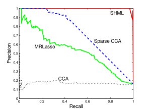
Figure 2: The precision-recall curves for association discovery.

The prediction accuracies on unknown ${\bf y}$ and their standard errors are shown in Figure 3. Our proposed SHML model achieves significant improvement over all the other methods. In particular, it reduces the prediction error of elastic net (which ranks the second best) by 25%, and reduces the error of LapSVM (which ranks the last), by 48%. Note that although utilizing the information from the unlabeled data, LapSMV lacks the capability to utilize underlying interaction structures and sparsify the model parameters, which may contribute its poor performance in the experiments.

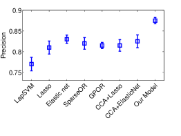
Figure 3: Prediction accuracies on the simulation data. The results are averaged over 10 runs.

In summary, the simulation results confirm the power of SHML in both discovering true associations between heterogeneous data sources and predicting unknown labels.

5.2 Study of Alzheimer’s Disease

We conducted association analysis and diagnosis of AD based on a dataset from Alzheimer’s Disease Neuroimaging Initiative(ADNI). The ADNI study is a longitudinal multisite observational study of elderly individuals with normal cognition, mild cognitive impairment, or AD. AD is the most common form of dementia with about 30 million patients worldwide and payments for care are estimated to be $200 billion in 2012.. In this analysis, we used SHML to study the associations of genotypes and brain atrophy measured by MRI and to predict the subject status (normal vs MCI vs AD). Note that the labels are ordinal since the three states represent increasing severity levels of the dementia.

The dataset was downloaded from http://adni.loni.ucla.edu/. After removing missing data, it consists 618 subjects (183 normal, 308 MCI and 134 AD), and for each patient, there are 924 SNPs (selected as the top SNPs to separate normal subjects from AD in ADNI) and 328 MRI features measuring the brain atrophies in different brain regions based on cortical thickness, surface area or volume using FreeSurfer software.

We compared SHML with the alternative methods on accuracy of predicting whether a subject is in the normal or MCI or AD condition. We randomly split the dataset into 556 training and 62 test samples 10 times and ran all the competing methods on each partition. As for the simulation study, we used the 10-fold cross validation for each run to tune free parameters. In SHML, in order to determine dimension $k$ for the latent representation ${\bf U}$, we computed the variational lower bounds as an approximation to the model marginal likelihood (i.e., evidence), with various $k$ values $\{10,20,40,60\}$. We chose the value with the largest approximate evidence, which led to $k=20$ (see Figure 4).

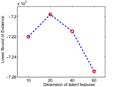
Figure 4: The variational lower bound for the model marginal likelihood.

Our experiments confirmed that with $k=20$, SHML achieved highest prediction accuracy, demonstrating the benefit of evidence maximization.

The accuracies for predicting unknown labels ${\bf y}$ and their standard errors are shown in Figure 5. Our method achieved the highest prediction accuracy, higher than that of the second best method, GP ordinal Regression, by 10% and than that of the worst method, CCA+lasso, by 22%.

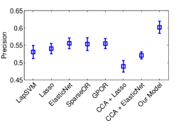
Figure 5: The prediction accuracy with standard errors on the real data.

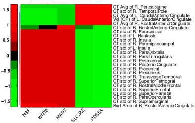
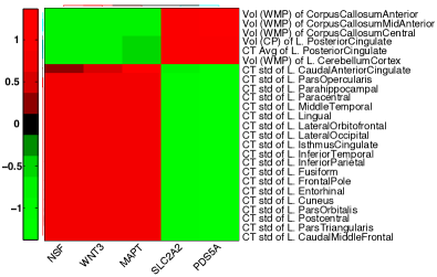
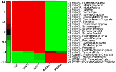
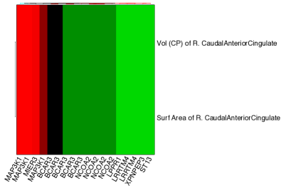
Figure 6: The estimated associations between MRI features and SNPs. In each sub-figure, the MRI features are listed on the right and the SNP names are given at the bottom.

We also examined the strongest associations discovered by SHML based on this dataset. First of all, the ranking of MRI features in terms of their prediction power of three different disease populations (normal, MCI and AD) demonstrate that most of top ranked features are based on the cortical thickness measurement. On the other hand, the features based on volume and surface area estimation of the same brain structures are less predictive. Particularly, thickness measurements of middle temporal lobe, precuneus, and fusiform were found to be most predictive compared with other brain regions. These findings are consistent with the memory-related function in these regions and findings in the literature for their prediction power of AD. We also found that measurements of the same structure on the left and right side have similar weights, indicating that the algorithm can automatically select correlated features in groups, since no asymmetrical relationship has been found for the brain regions involved in AD.

Secondly, the analysis of associating genotype to AD disease prediction also generated interesting results. Similar to the MRI features, SNPs that are in the vicinity of each other often listed together, indicating the group selection characteristics of the algorithm. For example, the top ranks SNPs are associated with a few genes including PSMC1P12 (proteasome 26S subunit, ATPase), NCOA2 (The nuclear receptor coactivator 2), and WDR52(WD repeat domain 52), which have been studied intensively in cancer research.

At last, biclustering of the gene-MRI association, as shown in Figure 6 reveal interesting pattern in terms of the relationship between genetic variations and brain atrophy measured by structural MRI. For example, the top ranks SNPs are associated with a few genes including BCAR3 (Breast cancer anti-estrogen resistance protein 3) and NCOA2, which have been studied more carefully in cancer research. One of the genes associated with this set of SNPs is MATP (microtubule-associated protein tau), which codes the tau gene that are associated closely with the AD. These findings reveal strong association between MATP gene and atrophy in the memory-related brain regions. Moreover, the same set of SNPs are also highly associated with cingulate, but in an opposite direction. These results indicate an opposite effect of genotype to the cingulate region, which is part of the limbic system and involve in emotion formation and processing, compared with other structures such as temporal lobe, which plays a more important role in the formation of long-term memory.

In summary, SHML discovered synergistic predictive relationships between brain atrophy, genetic variations and the disease status.

6 Conclusions

We have presented, SHML, a new Bayesian multiview learning framework. SHML simultaneously finds key associations between data sources (i.e., genetic variations and phenotypic traits) and to predict unknown ordinal labels. Experimental results on the ADNI data indicate that SHML found biologically meaningful associations between SNPs and MRI features and led to significant improvement on predicting the ordinal AD stages over the alternative classification and ordinal regression methods. Although we have focused on the AD study, we expect that SHML, as a powerful extension of CCA, can be applied to a wide range of applications in biomedical research – for example, eQTL analysis supervised by additional labeling information.

7 Acknowledgments

This work was supported by NSF IIS-0916443, NSF CAREER award IIS-1054903, and the Center for Science of Information (CSoI), an NSF Science and Technology Center, under grant agreement CCF-0939370.

References

- [1] L. Consoli et al. QTL analysis of proteome and transcriptome variations for dissecting the genetic architecture of complex traits in maize. Plant Mol Biol., 48(5):575–581, 2002.
- [2] D. Hunter. Lessons from genome-wide association studies for epidemiology. Epidemiology, (3):363–367, 2012.
- [3] S. Gandhi and N. Wood. Genome-wide association studies: the key to unlocking neurodegeneration? Nature Neuroscience, 13:789–794, 2010.
- [4] J. Liu et al. Combining fMRI and SNP Data to Investigate Connections Between Brain Function and Genetics Using Parallel ICA. Hum Brain Mapp., (1):1–30, 2009.
- [5] H. Harold. Relations between two sets of variates. Biometrika, 28:321–377, 1936.
- [6] F. Bach and M. Jordan. A probabilistic interpretation of canonical correlation analysis. Technical report, UC Berkeley, 2005.
- [7] E. Parkhomenko, D. Tritchler, and J. Beyene. Genome-wide sparse canonical correlation of gene expression with genotypes. BMC Proc., (Suppl 1), 2007.
- [8] M. Daniela and R. Tibshirani. Extensions of sparse canonical correlation analysis, with applications to genomic data. Statistical Applications in Genetics and Molecular Biology, 383(1), 2009.
- [9] X. Chen, H. Liu, and J. Carbonell. Structured sparse canonical correlation analysis. In AISTATS’12, volume 22, pages 199–207, 2012.
- [10] R. Tibshirani. Regression shrinkage and selection via the lasso. Journal of the Royal Statistical Society, Series B, 58:267–288, 1994.
- [11] H. Zou and T. Hastie. Regularization and variable selection via the elastic net. Journal of the Royal Statistical Society, Series B, 67:301–320, 2005.
- [12] M. Yuan and Y. Lin. Model selection and estimation in regression with grouped variables. Journal of the Royal Statistical Society, Series B, 68(1):49–67, 2007.
- [13] D. MacKay. Bayesian interpolation. Neural Computation, 4:415–447, 1991.
- [14] R. Neal. Bayesian Learning for Neural Networks. 1996.
- [15] P. Yu et al. Enriching amnestic mild cognitive impairment populations for clinical trials: optimal combination of biomarkers to predict conversion to dementia. Journal of Alzheimer’s Disease, 32(2):373–385, 2012.
- [16] L. Shen, Y. Qi, et al. Sparse bayesian learning for identifying imaging biomarkers in AD prediction. In Med Image Comput Comput Assist Interv., volume 13, pages 611–618, 2010.
- [17] E. George and R. McCulloch. Approaches for bayesian variable selection. Statistica Sinica, 7(2):339–373, 1997.
- [18] I. Goodfellow, A. Couville, and Y. Bengio. Large-scale feature learning with spike-and-slab sparse coding. In ICML’12. 2012.
- [19] S. Mohamed, K. Heller, and Z. Ghahramani. Bayesian and L1 approaches for sparse unsupervised learning. In ICML’02, 2012.
- [20] W. Chu and Z. Ghahramani. Gaussian processes for ordinal regression. Journal of Machine Learning Research, 6:1019–1041, 2005.
- [21] M. Braskie et al. Plaque and tangle imaging and cognition in normal aging and Alzheimer’s diseasee. Neurobiology of AgingArchives of Neurology, 31(10):1669–1678, 2010.
- [22] J. Zhou, J. Liu, V. Narayan, and J. Ye. Modeling disease progression via fused sparse group lasso. In KDD’12, pages 1095–1103, 2012.
- [23] L. Yuan, Y. Wang, P. Thompson, V. Narayan, and J. Ye. Multi-source learning for joint analysis of incomplete multi-modality neuroimaging data. In KDD’12, pages 1149–1157, 2012.
- [24] M. Beal. Variational Algorithms for Approximate Bayesian Inference. Ph.d. thesis, Gatsby Computational Neuroscience Unit, University College London, 2003.
- [25] M. Tipping and C. Bishop. Probabilistic principal component analysis. Journal of The Royal Statistical Society Series B-statistical Methodology, 61:611–622, 1999.
- [26] F. Bach and M. Jordan. A probabilistic interpretation of canonical correlation analysis. Technical report, UC Berkley, 2005.
- [27] Y. Guan and J. Dy. Sparse probabilistic principal component analysis. Journal of Machine Learning Research - Proceedings Track, 5:185–192, 2009.
- [28] S. Yu, K. Yu, V. Tresp, H. Kriegel, and M. Wu. Supervised probabilistic principal component analysis. In KDD’06, pages 464–473, 2006.
- [29] C. Archambeau and F. Bach. Sparse probabilistic projections. In Advances in Neural Information Processing Systems 21, pages 73–80. 2009.
- [30] S. Virtanen, A. Klami, and S. Kaski. Bayesian CCA via group sparsity. In ICML’11, pages 457–464, June 2011.
- [31] M. Titsias and M. Lázaro-Gredilla. Spike and slab variational inference for multi-task and multiple kernel learning. In NIPS’11, pages 2339–2347, 2011.
- [32] C. Carvalho, J. Chang, J. Lucas, JR Nevins, Q. Wang, and M. West. High-dimensional sparse factor modeling: applications in gene expression genomics. Journal of the American Statistical Association, 103(484):1438–1456, 2008.
- [33] D. Hardoon, G. Leen, S. Kaski, and J. Shawe-Taylor, editors. NIPS Workshop on Learning from Multiple Sources, 2008.
- [34] I. Rish, G. Grabarnik, G. Cecchi, F. Pereira, and G. Gordon. Closed-form supervised dimensionality reduction with generalized linear models. In ICML’08, pages 832–839, 2008.
- [35] J. Rupnik and J. Shawe-Taylor. Multi-view canonical correlation analysis. In KDD’10, 2010.
- [36] L. Sun, S. Ji, and J. Ye. Canonical correlation analysis for multi-label classification: A least squares formulation, extensions and analysis. IEEE Transactions on Pattern Analysis and Machine Intelligence, 33(1):194–200, 2011.
- [37] S. Kim, K. Sohn, and E. Xing. A multivariate regression approach to association analysis of a quantitative trait network. Bioinformaics, 25(12):204–212, 2009.
- [38] S. Melacci and B. Mikhail. Laplacian support vector machines trained in the primal. Journal of Machine Learning Research, 12:1149–1184, March 2011.