Tension, rigidity and preferential curvature of

interfaces between coexisting polymer solutions

R.H. Tromp^1,2 and E.M. Blokhuis³

¹NIZO food research, Kernhemseweg 2, 6718 ZB Ede, The Netherlands

²University of Utrecht, Department of Chemistry,

Padualaan 8, 3584 CH Utrecht, The Netherlands

³Colloid and Interface Science, Leiden Institute of Chemistry,

Gorlaeus Laboratories, P.O. Box 9502, 2300 RA Leiden, The Netherlands

Abstract

The properties of the interface in a phase-separated solution of polymers with different degrees of polymerization and Kuhn segment lengths are calculated. The starting point is the planar interface, the profile of which is calculated in the so-called ‘blob model’, which incorporates the solvent in an implicit way. The next step is the study of a metastable droplet phase formed by imposing a chemical potential different from that at coexistence. The pressure difference across the curved interface, which corresponds to this higher chemical potential, is used to calculate the curvature properties of the droplet. Interfacial tensions, Tolman lengths and rigidities are calculated and used for predictions for a realistic experimental case. The results suggest that interfaces between phase-separated solutions of polymers exhibit, in general, a preferential curvature, which stabilizes droplets of low molecular mass polymer in a high molecular mass macroscopic phase.

 

1 Introduction

When two chemically different liquid polymers are mixed, in the majority of cases phase separation takes place, because of the low gain in entropy after mixing, easily overruled by an adverse enthalpy of mixing. The presence of a common solvent usually suppresses the drive to phase separate, but only when the solvent is present at volume fractions of typically 90% or more. When the solvent is present at a lower concentration, phase separation takes place, giving rise to phase regions differing in polymer composition and total polymer concentration. The driving force for the phase separation is a repulsive, possibly entropic, force between the polymers, or a difference in the quality of the solvent for the two polymers [1]. Phase separation in a polymer mixture can also occur such that the polymers reside in one phase and the solvent in the other (complex coacervation).

Interfaces between phases of coexisting, thermodynamically incompatible polymer solutions are referred to as solvent-solvent interfaces. An example is phase-separated protein and (neutral) polysaccharide solutions found in food systems [2]. The solvent-solvent interface, in that case a water-water interface, is then situated between the coexistent protein-rich and polysaccharide-rich solutions. The interfacial tension of solvent-solvent interfaces is extremely low (typically a few $\mu$N/m or less) so that the interface is highly deformable, e.g. by convective flows, and therefore difficult to investigate by classical methods (such as the Wilhelmy plate method). Methods to estimate the interfacial tension are capillary rise [3], spinning drop [4, 5, 7, 6], shape relaxation after deformation [8, 9, 10], or by manipulation with a laser beam [11].

The macroscopic phase separation takes place via a stage in which one phase is a dispersion of microscopic droplets in a continuous matrix of the other phase. This state might be called a solvent-solvent emulsion. Figure 1 gives an example. Such an emulsion is often surprisingly stable. This may be because of the small density difference (both phases are typically 90% solvent), low interfacial tension or the existence of a preferential curvature. In order to get a basic theoretical understanding of the properties that play a role in the stability of such solvent-solvent emulsions, we present calculations of the interfacial tension, preferential curvature and rigidity of equilibrium and quasi-equilibrated curved interfaces between polymer phases. This is done using the so called ’blob model’ [12]. The blob model is based on a Flory-Huggins mean-field approach but it is adapted to include excluded volume fluctuations which are correlated over a blob size (correlation length) $\xi$. Since solvent-solvent interfaces are wide, it contains only weak gradients so that it seems appropriate to describe the interfacial region in terms of the van der Waals squared-gradient expansion.

In this article, we discuss two simplified cases: (i) identical degrees of polymerization and solvent qualities, but allowing for a solvent gradient in the interface, (ii) different degrees of polymerization and solvent qualities (i.e. different Kuhn lengths), but neglecting the solvent gradient in the interface. Case (i) was previously treated by Broseta et al. [13, 14, 15] and will be used as an introduction to case (ii). A preferential curvature is expected in case (ii) because the energy in the compositional gradient depends on the blob size ratio and the ratio of the number of blobs per chain.

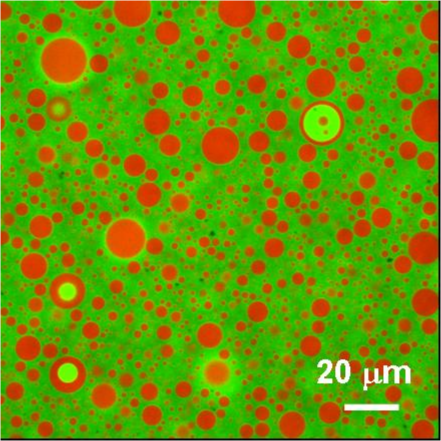
Figure 1: Water-water emulsion, from a phase separated aqueous solution of 10% fish gelatin (non-gelling), and 10% dextran (200 kDa). Light phase: gelatin-rich; dark phase: dextran-rich.

2 The blob model

2.1 Approach by Broseta et al.

The derivation of Broseta et al. [13, 14, 15, 16] starts with the Flory Huggins model [17] for an isotropic polymer melt consisting of two polymer types of equal length $N$. We denote the volume fractions of type A and type B as $\phi_{A}\!=\!\phi$ and $\phi_{B}\!=\!1-\phi$. Then,

$$\frac{F_{\rm FH}(\phi)}{V\,k_{\rm B}T}=\frac{1}{a^{3}}\left[\frac{\phi}{N}\,\ln(\phi)+\frac{(1-\phi)}{N}\,\ln(1-\phi)+\chi\,\phi\,(1-\phi)\right]\,,$$ (1)

where $a$ is the dimension of the lattice which equals the Kuhn segment length. The Flory parameter $\chi$ represents the interaction between the two polymer types.

The Flory-Huggins model is used by Broseta et al. [14] for a mixture of two polymers well above the overlap concentration (semi-dilute solution) in a solvent which is a good solvent for both polymers. In that situation the blob model can be used to describe the polymer solution [12]. The blob model incorporates the effect of fluctuations due to excluded volume interactions by replacing the Kuhn segment length $a$ by a ‘blob size’ $\xi$ and the polymer length $N$ by the number of blobs, $N_{b}\!=\!N/(c\,\xi^{3})$ per polymer chain:

$$\frac{F_{\rm blob}(\phi,c)}{V\,k_{\rm B}T}=\frac{1}{\xi^{3}}\left[\frac{\phi}{N_{b}}\,\ln(\phi)+\frac{(1-\phi)}{N_{b}}\,\ln(1-\phi)+u\,\phi\,(1-\phi)+K\right]\,,$$ (2)

where $K\!=\!0.024$ is a constant [13, 15], related to the osmotic pressure, and where $u$ represents the interaction between blobs of type A and B. The whole volume is now filled by ‘blobs’ of dimension $\xi$ with each ‘blob’ either containing polymer of type A or type B. An essential feature in the blob model is that both the blob size $\xi\!=\!\xi(c)$ and the interaction parameter $u\!=\!u(c)$ depend on the (total) monomer concentration $c$ [12, 18]:

$$\xi(c)\simeq 0.43\,R_{\rm g}\left(\frac{c}{c^{*}}\right)^{-\nu/(3\nu-1)}\,,$$ (3)

and

$$u(c)=u_{\rm crit}\left(\frac{c}{c_{\rm crit}}\right)^{\chi/(3\nu-1)}\,,$$ (4)

where the exponents $\nu\!=$ 0.60 and $\chi\!=$ 0.22 are such that non-mean-field chain statistics is explicitly taken into account ($\chi$ can be interpreted as the number of monomeric contacts between overlapping blobs). Furthermore, $c^{*}$ is the overlap concentration, $R_{\rm g}$ the polymer radius of gyration in dilute (non-overlapping) conditions, and $u_{\rm crit}$ is the interaction at a reference concentration, for which we shall take the critical demixing concentration, $c_{\rm crit}$.

The blob model for an isotropic polymer mixture can be extended to non-homogeneous polymer solutions. This is achieved by allowing $\phi\!=\!\phi(\vec{r})$ and $c\!=\!c(\vec{r})$ to be position dependent and by adding squared gradient terms to the free energy:

$$\frac{F[\phi,c]}{k_{\rm B}T} = \int\!\!d\vec{r}\left[\frac{\phi}{N_{b}\,\xi^{3}}\,\ln(\phi)+\frac{(1-\phi)}{N_{b}\,\xi^{3}}\,\ln(1-\phi)+\frac{u}{\xi^{3}}\,\phi\,(1-\phi)\right.$$ (5)

$$\left.+\frac{K}{\xi^{3}}+\frac{|\vec{\nabla}\phi|^{2}}{24\,\xi\,\phi}+\frac{|\vec{\nabla}\phi|^{2}}{24\,\xi\,(1-\phi)}+\frac{|\vec{\nabla}c|^{2}}{24\,\xi\,c^{2}}\right]\,.$$

This expression is used by Broseta et al. [14] to determine density profiles and surface tension of a planar interface. We revisit their analysis in the Appendix and point to some small errors in their original formulas.

We can extend the above free energy to non-symmetric polymer solutions by allowing the blob size and number of blobs to differ for each polymer type. This may be due to a different degree of polymerization, different solvent qualities, different Kuhn lengths, etc. The difference in blob size ($\xi_{A}$ and $\xi_{B}$) and number of blobs ($N_{b,A}$ and $N_{b,B}$), then leads to the following modification of the expression for the free energy:

$$\frac{F[\phi,c]}{k_{\rm B}T} = \int\!\!d\vec{r}\left[\frac{\phi}{N_{b,A}\,\xi_{A}^{3}}\,\ln(\phi)+\frac{(1-\phi)}{N_{b,B}\,\xi_{B}^{3}}\,\ln(1-\phi)+\frac{u}{\xi^{3}}\,\phi\,(1-\phi)\right.$$ (6)

$$\left.+\frac{K}{\xi^{3}}+\frac{|\vec{\nabla}\phi|^{2}}{24\,\xi_{A}\,\phi}+\frac{|\vec{\nabla}\phi|^{2}}{24\,\xi_{B}\,(1-\phi)}+\frac{|\vec{\nabla}c|^{2}}{24\,\xi\,c^{2}}\right]\,,$$

where we have defined an effective blob size as

$$\frac{1}{\xi}=\frac{1}{2}\left(\frac{1}{\xi_{A}}+\frac{1}{\xi_{B}}\right)\,.$$ (7)

The form of the free energy in Eq.(6) is derived by replacing $\xi\!\rightarrow\!\xi_{A/B}$ and $N_{b}\!\rightarrow\!N_{b,A/B}$ in the corresponding terms in the free energy in Eq.(5). For the other terms in Eq.(5), such as the term describing the interaction between blobs, the blob size is replaced by an effective blob size which should somehow be related to the two blob sizes $\xi_{A}$ and $\xi_{B}$. We have chosen the expression in Eq.(7) to calculate the effective blob size since it reduces to $\xi$ for the symmetric polymer system and because its value is dominated by the smallest of the two blob sizes. Naturally, other models for the free energy may be constructed and, in particular, one may propose a different expression to calculate the effective correlation length, but we expect that most of the physics involved is captured by the expression for the free energy in Eq.(6).

In the following sections, this free energy is applied to study spherically (and cylindrically) shaped droplets. In the next section, we assume that we can neglect the variation of the total monomer concentration profile in the interfacial region and assume that $c(\vec{r})\!=\!c$ everywhere.

2.2 Calculation of the curved interface profile

When we neglect the variation of the total monomer concentration, we have that $c(\vec{r})\!=\!c$ and we may replace both the blob size and the interaction parameter by their constant values in the bulk region: $\xi\!\rightarrow\!\bar{\xi}$ and $u\!\rightarrow\!\bar{u}$ (the bar denotes the corresponding bulk value). Furthermore, the free energy is a functional of $\phi(\vec{r})$ only and we can write for the grand free energy:

$$\Omega[\phi]=\int\!\!d\vec{r}\left[f(\phi)-\mu\,\phi+m(\phi)\,|\vec{\nabla}\phi|^{2}\right]\,,$$ (8)

where we have defined

$$f(\phi)=\frac{\bar{u}\,k_{\rm B}T}{\bar{\xi}^{3}}\left[\frac{2\phi}{(1+\alpha)\,\omega}\,\ln(\phi)+\frac{2\alpha\,(1-\phi)}{(1+\alpha)\,\omega}\,\ln(1-\phi)-\phi^{2}\right]\,,$$ (9)

and

$$m(\phi)=\frac{k_{\rm B}T\,(1+(r_{0}-1)\phi)}{12\,\bar{\xi}\,(1+r_{0})\phi(1-\phi)}\,,$$ (10)

with the two asymmetry parameters $\alpha$ and $r_{0}$ defined as:

$$\alpha\equiv\frac{\bar{N}_{b,A}\,\bar{\xi}_{A}^{3}}{\bar{N}_{b,B}\,\bar{\xi}_{B}^{3}}\,,$$ (11)

and

$$r_{0}\equiv\frac{\bar{\xi}_{A}}{\bar{\xi}_{B}}\,.$$ (12)

The parameter $\alpha$ represents the difference in degree of polymerization of the two polymers, while $r_{0}$ reflects the difference in Kuhn lengths, e.g. due to a difference in solvent quality or chain stiffness. The dimensionless interaction parameter $\omega$ is defined by

$$\omega\equiv\frac{2\bar{u}}{\bar{\xi}^{3}}\left(\frac{1}{\bar{N}_{b,A}\,\bar{\xi}_{A}^{3}}+\frac{1}{\bar{N}_{b,B}\,\bar{\xi}_{B}^{3}}\right)^{\!-1}\,,$$ (13)

which can also be written as:

$$\omega=\frac{(1+\sqrt{\alpha})^{2}}{1+\alpha}\,\left(\frac{c}{c_{\rm crit}}\right)^{(\chi+1)/(3\nu-1)}\,,$$ (14)

where we have used Eqs.(4) and (11) and the fact that $\omega_{\rm crit}\!=\!(1+\sqrt{\alpha})^{2}/(1+\alpha)$. This last expression will be used to link our theoretical results to more experimentally accessible quantities.

Next, we consider a spherically shaped droplet with (equimolar) radius $R$. The radius $R$ is really a radius of curvature and its sign is chosen such that a positive curvature corresponds to the phase rich in polymer $A$ (the ‘liquid’) residing inside the droplet with the (metastable) phase rich in polymer $B$ (the ‘vapor’) outside. As a consequence, $\alpha\!>\!1$ means that the degree of polymerization inside the droplet is larger than outside, and $r_{0}\!>\!1$ means that inside the droplet the characteristic length scale (blob size) is larger than outside. The equimolar radius $R$ of a liquid drop is defined in the expression:

$$4\pi\int\limits_{0}^{\infty}\!\!dr\;r^{2}\left[\,\phi(r)-\phi_{v}\right]=\frac{4\pi}{3}\,R^{3}\,(\phi_{\ell}-\phi_{v})\,.$$ (15)

The excess (grand) free energy of the metastable critical nucleus is defined as:

$$\frac{\Delta\Omega}{A}\equiv\frac{\Omega+p_{v}\,V}{A}=-\frac{\Delta p\,R}{3}+\sigma(R)\,,$$ (16)

with $p_{v}$ the vapour pressure outside the droplet and $p_{\ell}=p_{v}+\Delta p$ is the liquid pressure inside (see remark below, however). $A\!=\!4\pi\,R^{2}$ is the area of a droplet of radius $R$. The quantity $\sigma(R)$ is the surface tension of the droplet as a function of the radius $R$. This is the quantity that we wish to study and the above formula provides a way to determine it from $\Delta\Omega$.

In spherical geometry, the free energy in Eq.(8) is:

$$\frac{\Delta\Omega[\phi]}{A} = \int\limits_{0}^{\infty}\!\!dr\left(\frac{r}{R}\right)^{\!2}\left[f(\phi)-\mu\,\phi+p_{v}+m(\phi)\,\phi^{\prime}(r)^{2}\,\right]\,.$$ (17)

The Euler-Lagrange equation to minimize the above free energy is given by

$$2m(\phi)\,\phi^{\prime\prime}(r)=-\frac{4m(\phi)}{r}\,\phi^{\prime}(r)-m^{\prime}(\phi)\phi^{\prime}(r)^{2}+f^{\prime}(\phi)-\mu\,,$$ (18)

where the prime denotes a derivative with respect to its argument. The procedure to determine $\sigma(R)$ as a function of $R$ is now as follows: (1) We first determine the bulk densities $\phi_{0,\ell}$ and $\phi_{0,v}$ coexisting across a planar interface ($R\!=\!\infty$), which we refer to as the the state of coexistence. The corresponding value of the chemical potential is then denoted as $\mu_{\rm coex}$. Determination of $\mu_{\rm coex}$, $\phi_{0,\ell}$ and $\phi_{0,v}$ is achieved by solving the following set of equations for given $\omega$ and asymmetry parameters $\alpha$ and $r_{0}$:

$$f^{\prime}(\phi_{0,v}) = \mu_{\rm coex}\,,\hskip 25.0ptf^{\prime}(\phi_{0,\ell})=\mu_{\rm coex}\,,$$

$$f(\phi_{0,v})-\mu_{\rm coex}\,\phi_{0,v} = f(\phi_{0,\ell})-\mu_{\rm coex}\,\phi_{0,\ell}\equiv-p_{\rm coex}\,.$$ (19)

The resulting phase diagram is shown in Figure 2 for various values of $\alpha$.

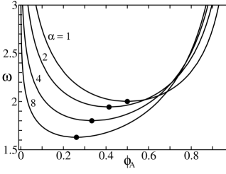
Figure 2: Polymer phase diagram of mixing for several asymmetry ratios $\alpha$, representing a difference in degree of polymerization (see Eq.(11)). $\omega$ is a dimensionless interaction parameter given in Eq.(14). The solid circles denote the locations of the critical demixing points, $\omega_{\rm crit}\!=\!(1+\sqrt{\alpha})^{2}/(1+\alpha)$, $\phi_{\rm crit}\!=\!1/(1+\sqrt{\alpha})$.

(2) Next, we vary the chemical potential $\mu$ to a value off-coexistence. The consequence of choosing a value of $\mu$ different from $\mu_{\rm coex}$ is the coexistence of two pressures across a curved interface. In the simplest case of spherical droplets we have droplets of liquid ($R\!>\!0$) for $\mu\!>\!\mu_{\rm coex}$ and droplets of vapour ($R\!<\!0$) for $\mu\!<\!\mu_{\rm coex}$. For given $\mu$, $\omega$ and $\alpha$ the densities $\phi_{\ell}$ and $\phi_{v}$ are determined from solving the following two equations:

$$f^{\prime}(\phi_{v})=\mu\,,\hskip 25.0ptf^{\prime}(\phi_{\ell})=\mu\,,$$ (20)

with the corresponding bulk pressures calculated from

$$f(\phi_{v})-\mu\,\phi_{v}=-p_{v}\,,\hskip 25.0ptf(\phi_{\ell})-\mu\,\phi_{\ell}=-p_{\ell}\,.$$ (21)

It should be noted that far outside the droplet ($r\!\rightarrow\!\infty$) the density (or pressure) becomes equal to that of the bulk, $\phi(\infty)\!=\!\phi_{v}$, but that only for a very large droplet is the density (or pressure) inside the droplet ($\phi(0)$) equal to the bulk ($\phi_{\ell}$). (3) As a next step, the Euler-Lagrange equation for $\phi(r)$ in Eq.(18) is solved numerically with the boundary condition $\phi(\infty)\!=\!\phi_{v}$. The resulting density profile $\phi(r)$ thus obtained is finally inserted into Eq.(15) to determine $R$ and into Eq.(17) to determine $\Delta\Omega$ and thus $\sigma(R)$.

In Figure 3, two examples of $\sigma(R)$ are shown as a function of $1/R$. These quantities are shown in reduced units which are such that all energies are in units of $k_{\rm B}T/6(6\bar{u})^{\frac{1}{2}}$ and all lengths are in units of $D_{\infty}\!\equiv\!\bar{\xi}/(6\bar{u})^{\frac{1}{2}}$, which is the interfacial width at infinite incompatibility of the two polymers, i.e. at infinite degree of polymerization [14]. This means that the surface tension and radius in reduced units are:

$$\tilde{\sigma}(R) \equiv \frac{\bar{\xi}^{2}}{k_{\rm B}T\,(\bar{u}/6)^{\frac{1}{2}}}\,\sigma(R)\,,$$ (22)

$$\tilde{R} \equiv \frac{R}{D_{\infty}}=\frac{(6\bar{u})^{\frac{1}{2}}}{\bar{\xi}}\,R\,.$$

The determination of $\sigma(R)$ is quite elaborate and most of the time we are only interested in its general shape. For this reason we perform a curvature expansion in $1/R$ in the next section to determine the parabolic approximation to $\sigma(R)$ shown as the solid line in Figure 3.

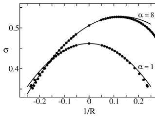
Figure 3: Surface tension of a spherical droplet as function of $1/R$, for ratios of degree of polymerization $\alpha=$ 1 and 8. For the reduced units, see Eq.(22). $R\!>\!0$ corresponds to droplets of the phase rich in polymer $A$ and $R\!<\!0$ corresponds to droplets of the phase rich in polymer $B$. We have set $\omega=$ 4 and $r_{0}=$ 1 (equal blob sizes). The solid lines are parabolic approximations to $\sigma(R)$ determined from the curvature expansion.

2.3 Curvature expansion

We can analyze the results in the previous section by performing a curvature expansion in $1/R$. All quantities are then expanded in $1/R$. For the density profile and surface tension, for instance, we have:

$$\phi(r) = \phi_{0}(z)+\frac{\phi_{1}(z)}{R}+\ldots\,,$$

$$\sigma(R) = \sigma-\frac{2\delta\sigma}{R}+\frac{2k+\bar{k}}{R^{2}}+\ldots\,,$$ (23)

where $z\!\equiv\!r-R$ and where $\sigma$ is the surface tension of the planar interface, $\delta$ is the Tolman length [19], related to the radius of spontaneous curvature as $R_{0}=2k/\delta\sigma$ [20], $k$ is the bending rigidity and $\bar{k}$ is the rigidity constant associated with Gaussian curvature [21]. An expansion of the Euler-Lagrange equation in Eq.(18) yields to zeroth order:

$$m(\phi_{0})\,\phi_{0}^{\prime}(z)^{2}=f(\phi_{0})-\mu_{\rm coex}\,\phi_{0}(z)+p_{\rm coex}\,.$$ (24)

Expansion of the Euler-Lagrange equation to first order gives:

$$2m(\phi_{0})\,\phi_{1}^{\prime\prime}(z) = -4m(\phi_{0})\,\phi_{0}^{\prime}(z)-\mu_{1}-2m^{\prime}(\phi_{0})\,\phi_{0}^{\prime}(z)\phi_{1}^{\prime}(z)$$

$$+\phi_{1}(z)\left[f^{\prime\prime}(\phi_{0})-2m^{\prime}(\phi_{0})\,\phi_{0}^{\prime\prime}(z)-m^{\prime\prime}(\phi_{0})\,\phi_{0}^{\prime}(z)^{2}\,\right]\,.$$

with $\mu_{1}\!=\!2\sigma/(\phi_{0,\ell}-\phi_{0,v})$ [22, 23]. One may show [22] that the coefficients in the expansion of $\sigma(R)$ in Eq.(2.3) can be written in terms of the density profiles $\phi_{0}(z)$ and $\phi_{1}(z)$:

$$\sigma = \int\limits_{-\infty}^{\infty}\!\!\!dz\;2m(\phi_{0})\,\phi_{0}^{\prime}(z)^{2}\,,$$

$$\sigma\delta = -\int\limits_{-\infty}^{\infty}\!\!\!dz\;2m(\phi_{0})\,z\,\phi_{0}^{\prime}(z)^{2}\,,$$ (26)

$$2k+\bar{k} = \int\limits_{-\infty}^{\infty}\!\!\!dz\left[2m(\phi_{0})\,z^{2}\,\phi_{0}^{\prime}(z)^{2}-2m(\phi_{0})\,\phi_{1}(z)\phi_{0}^{\prime}(z)+\mu_{1}z^{2}\,\phi_{0}^{\prime}(z)+\frac{\mu_{1}}{2}z\,\phi_{1}^{\prime}(z)\right]\,.$$

The surface tension and Tolman length are independent of the choice for the location of the interface (the position of the $z\!=\!0$ plane) but $k$ and $\bar{k}$ do depend on this choice. For all of the above expressions we have taken the equimolar radius for $R$, see Eq.(15), which implies that the planar density profile obeys

$$\int\limits_{-\infty}^{\infty}\!\!\!dz\;z\,\phi_{0}^{\prime}(z)=0\,.$$ (27)

The same expansion can be carried out for a cylindrical interface. For the density profile and surface tension one then has instead of Eq.(2.3):

$$\phi(r) = \phi_{0}(z)+\frac{\phi_{1}(z)}{2R}+\ldots\,,$$

$$\sigma(R) = \sigma-\frac{\delta\sigma}{R}+\frac{k}{2R^{2}}+\ldots\,.$$ (28)

This gives us the opportunity to determine $k$ and $\bar{k}$ separately with the result [22]

$$\bar{k} = \int\limits_{-\infty}^{\infty}\!\!\!dz\;2m(\phi_{0})\,z^{2}\,\phi_{0}^{\prime}(z)^{2}\,,$$

$$k = \int\limits_{-\infty}^{\infty}\!\!\!dz\left[-m(\phi_{0})\,\phi_{1}(z)\phi_{0}^{\prime}(z)+\frac{\mu_{1}}{2}z^{2}\,\phi_{0}^{\prime}(z)+\frac{\mu_{1}}{4}z\,\phi_{1}^{\prime}(z)\right]\,.$$ (29)

The procedure to determine the curvature coefficients $\sigma$, $\delta$, $k$ and $\bar{k}$ is now as follows: (1) The planar profile $\phi_{0}(z)$ is first determined from the differential equation in Eq.(24) with $\phi_{0,\ell}$, $\phi_{0,v}$, $\mu_{\rm coex}$ and $p_{\rm coex}$ determined from the set of equations in Eq.(2.2). (2) The location of the $z\!=\!0$ plane is chosen such that Eq.(27) is satisfied. This location depends on the asymmetry of the interface profile. (3) With $\phi_{0}(z)$ determined, $\sigma$, $\delta$ and $\bar{k}$ can all be evaluated from the integrals in Eqs.(2.3) and (2.3). (4) The constant $\mu_{1}$ is subsequently determined from $\mu_{1}\!=\!2\sigma/(\phi_{0,\ell}-\phi_{0,v})$ which allows us to determine the bulk density values $\phi_{1,\ell/v}$ from $\phi_{1,\ell/v}\!=\!\mu_{1}/f^{\prime\prime}(\phi_{0,\ell/v})$. (5) For given $\phi_{0}(z)$ and $\mu_{1}$, the differential equation for $\phi_{1}(z)$ in Eq.(2.3) may now be solved with the boundary conditions $\phi_{1}(-\infty)\!=\!\phi_{\ell}$ and $\phi_{1}(\infty)\!=\!\phi_{v}$. One may verify that if $\phi_{1}(z)$ is particular solution of Eq.(2.3) then also $\phi_{1}(z)+{\rm constant}\cdot\phi^{\prime}_{0}(z)$ is also a solution. It turns out that $k$ is independent of the value of this integration constant so we may arbitrarily take $\phi_{1}(0)\!=\!0$ for convenience [24]. (6) Finally, with $\phi_{1}(z)$ determined, $k$ (or $2k+\bar{k}$) can be evaluated from the integral in Eq.(2.3).

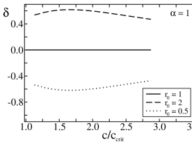
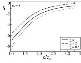
Figure 4: Variation of the Tolman length (in nm) as a function of monomer concentration for two ratios of the degree of polymerization and three ratios of the blob size.

The result of this procedure for the Tolman length is shown in Figure 4 for various values of $\alpha$ and $r_{0}$. For a perfectly symmetric profile ($\alpha\!=\!1$ and $r_{0}\!=\!1$) we have that $\delta\!=\!0$ identically: there is no preferred curvature to either phase. When $\alpha\!>\!1$, we obtain negative values for $\delta$ indicating that the droplets of the phase rich in A ($R\!>\!0$) have a higher surface tension as compared to droplets rich in polymer B ($R\!<\!0$). This feature can also be seen from the graph in Figure 3. The influence of $r_{0}$ is less pronounced with $r_{0}\!>\!1$ leading to a positive contribution and $r_{0}\!<\!1$ leading to a negative contribution to $\delta$.

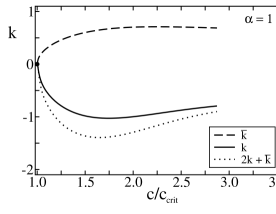
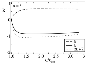
Figure 5: Variation of the rigidities (in units of $k_{\rm B}T$) as a function of monomer concentration for two ratios of the degree of polymerization. $k$ is the bending rigidity and $\bar{k}$ is the rigidity constant associated with Gaussian curvature.

In Figure 5, we show the rigidity constants $k$ and $\bar{k}$ and the combination $2k+\bar{k}$ in units of $k_{\rm B}T$ for $\alpha\!=\!1$ and for $\alpha\!=\!8$. It is noted that $2k+\bar{k}$ is negative indicating that $\sigma(R)$ as a function of $1/R$ has a negative second derivative, cf. Figure 3.

3 Discussion

In this section, we discuss in more detail the symmetric polymer system for which the actual numbers quoted in Figures 4 and 5 are derived. The bar to denote bulk values shall be omitted in this section. We first consider the symmetric, planar interface as treated by Broseta et al. [13, 14, 15].

3.1 Symmetric polymer system

For the symmetric polymer system, the influence of the solvent on the interfacial tension of the planar interface can be investigated using the approach of Broseta et al. [13, 14, 15], detailed in the Appendix. In order to make the connection with experiments, we consider the parameters typical for aqueous solutions of gelatin and dextran [16], which have a radius of gyration $R_{\rm g}\simeq$ 18 nm, degree of polymerisation $N\simeq$ 1000, and molecular mass of the monomers, $M_{\rm mon}\simeq$ 120 g mol^-1. The overlap concentration $c^{*}$ may then be estimated from

$$c^{*}\simeq\frac{N}{(4\pi/3)R_{\rm g}^{3}}\,,$$ (30)

which gives $c^{*}\simeq$ 0.82% mass per mass solution. By convention, we shall write concentrations in units of % mass per mass solution which is achieved by multiplying the concentration expressed as number of molecules per volume by the molecular mass and dividing by Avogadro’s number and the solvent (water) mass density.

The blob size $\xi$ in this symmetric polymer system can be calculated as a function of the bulk monomer concentration $c$ using Eq.(3) [18]:

$$\xi(c)\simeq 0.43\,R_{\rm g}\left(\frac{c}{c^{*}}\right)^{-\nu/(3\nu-1)}\,.$$ (31)

From the blob size, the number of blobs per chain as a function of the total monomer concentration is then determined from:

$$N_{\rm b}(c)=\frac{N}{c\,\xi(c)^{3}}\,.$$ (32)

For the polymer solution consisting of gelatin and dextran, the critical demixing concentration is estimated as $c_{\rm crit}\simeq$ 3.5% mass per mass solution. The blob size at the critical concentration can then be estimated from Eq.(31), giving $\xi_{\rm crit}\simeq$ 2.6 nm, and the number of blobs per chain at the critical demixing concentration is estimated from Eq.(32) as $N_{\rm b,crit}\simeq$ 325.

By choosing in Eq.(4) the critical concentration of demixing as the reference concentration, $u$ also becomes experimentally accessible:

$$u(c)=\frac{\omega_{\rm crit}}{N_{\rm b,crit}}\left(\frac{c}{c_{\rm crit}}\right)^{\!\chi/(3\nu-1)}\,,$$ (33)

where we have used that $\omega\!=\!N_{\rm b}u$ [14]. For the symmetrical polymer system ($\alpha\!=\!1$), we have that $\omega_{\rm crit}\!=$ 2, which gives $u_{\rm crit}\!\simeq$ 0.0061. In Table 1, we list the values of the parameters of the gelatin-dextran system together with the parameters calculated from these numbers and their range when the monomer concentration is varied between $c\!=$ 3.5% (w/w) and $c\!=$ 10% (w/w).

quantity		value
$R_{\rm g}$	radius of gyration	18 nm
$N$	degree of polymerisation	1000
$M_{\rm mon}$	monomer molecular mass	120 g mol-1
$c^{*}$	monomer overlap concentration	0.82% (w/w)
$c_{\rm crit}$	critical demixing concentration	3.5% (w/w)
$\xi_{\rm crit}$	critical blob size	2.6 nm
$N_{\rm b,crit}$	critical number of blobs per chain	325
$u_{\rm crit}$	critical interaction parameter	0.0061
$c$	monomer concentration	3.5-10% (w/w)
$\xi$	blob size	2.6-1.2 nm
$N_{\rm b}$	number of blobs per chain	325-1200
$u$	interaction parameter	0.0061-0.0084

Table 1: Values of the parameters of the gelatin-dextran system [16] and their variation with monomer concentration $c$.

The free energy by Broseta et al. in Eq.(5) for the symmetric polymer system takes into account the reduction of the monomer concentration by the accumulation of solvent at the interface, which is ignored in the calculation of the properties of non-symmetric interfaces. It is therefore useful to first consider the relevance of this effect. This can be done by plotting the ratio of the interfacial tension of the planar interface calculated with and without taking the reduction due to the solvent redistribution into account. This ratio is (see Eq.(48)):

$$\Theta\equiv\frac{\sigma_{c=c(z)}}{\sigma_{c=\rm constant}}=\frac{1-\Delta_{1}-u\,\Delta_{2}}{1-\Delta_{1}}\,.$$ (34)

It turns out that the effect of solvent redistribution is significant in the whole concentration range, reducing the interfacial tension by at least 20% (See Figure 6).

Figure 6: Ratio of the interfacial tension corrected and not corrected for the effect of solvent redistribution as a function of the (bulk) monomer concentration. In this example, we have set $u\!=$ 0.05.

However, the reduction is nearly constant above a monomer concentration of 1.5 $c_{\rm crit}$ ($\omega\apprge$ 3.7), above which the decreasing amount of solvent is compensated by the increasing segregation of the polymers at the interface. It is tentatively assumed that calculations which ignore the solvent become more reliable at increasing monomer concentration. The properties of the curved interface should therefore be considered only at $\omega\apprge$ 4.

3.2 Asymmetric polymer system

In our theoretical analysis, the Tolman length and rigidity constants are calculated, as a function of the dimensionless interaction parameter $\omega$, in reduced units similar to those in Eq.(22):

$$\tilde{\delta}\equiv\frac{\delta}{D_{\infty}}=\frac{(6u)^{\frac{1}{2}}}{\xi}\,\delta\hskip 25.0pt{\rm and}\hskip 25.0pt\tilde{k}\equiv\frac{6(6u)^{\frac{1}{2}}}{k_{\rm B}T}\,k\,.$$

To transform these units into experimentally relevant values, we need to make assumptions on the value of the effective blob size $\xi$ (Eq.(7)) and the blob interaction parameter $u$ (Eq.(13)) also for the asymmetric polymer system. [The value and concentration dependence of $\omega$ is given by Eq.(14).] Since the concentration dependence of $\xi$ and $u$ is the same as in Eqs.(31) and (33), we therefore only need to assume values for their critical values $\xi_{\rm crit}$ and $u_{\rm crit}$. As a first guess, it seems appropriate to assign for $\xi_{\rm crit}$ and $u_{\rm crit}$, the same values as in the symmetric case, $\xi_{\rm crit}\!\simeq$ 2.6 nm and $u_{\rm crit}\!\simeq$ 0.0061.

The Tolman length (Figure 4) is, as obtained before [23], in the range of nanometers. The Tolman length is related to a preferential curvature of the interface and it can differ from zero because of unequal degrees of polymerization or because of unequal blob sizes. For a prediction of the sign of the Tolman length for a specific pair of polymers, one therefore needs to know the molecular mass ratio and the respective Kuhn lengths.

The implications of the sign of the Tolman length are apparent in Figure 3 which shows the interfacial tension as a function of radius of curvature for a symmetric and asymmetric polymer system. According to the definition of the asymmetry parameter $\alpha$ in Eq.(11), the droplet phase has a higher degree of polymerization than the surrounding infinite phase when $\alpha\!>\!1$. Therefore, the shape of $\sigma(R)$ as a function of $1/R$ in Figure 3 implies that in a phase-separated polymer mixture, a droplet of high molecular mass has a higher surface energy than a droplet of low molecular mass. This would imply that the formation of droplets of the lower molecular mass is energetically more favourable.

3.3 Droplet stability

To elucidate the role of the radius dependent surface tension on the stability of the droplets, we consider the free energy of a dispersion of $N_{s}$ spherical droplets with radius $R$:

$$\Omega(N_{s},R)=N_{s}\,4\pi R^{2}\,\left[\,\sigma-\frac{2\delta\sigma}{R}+\frac{2k+\bar{k}}{R^{2}}\,\right]-\Delta p\,N_{s}\,\frac{4\pi}{3}R^{3}\,.$$ (35)

The above free energy should be minimized with respect $N_{s}$ and $R$ keeping the total volume of the particles, $V_{0}\!=\!\,N_{s}\,(4\pi/3)R^{3}$, fixed. This yields the Laplace equation for the pressure difference:

$$\Delta p=\frac{2\sigma}{R}-\frac{2\delta\sigma}{R^{2}}\,,$$ (36)

and we obtain for the preferential radius:

$$R_{\rm pref}=2\delta+\left(4\delta^{2}-\frac{3}{\sigma}(2k+\bar{k})\right)^{\!\frac{1}{2}}\,.$$ (37)

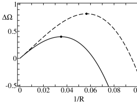
Figure 7: Excess free energy density relative to the planar state $\Delta\Omega$ (in units of $k_{\rm B}T$/(10 nm)³) as a function of the inverse radius (in units of nm^-1). The solid line corresponds to droplets containing low molecular mass polymer surrounded by a continuous phase consisting of the high molecular mass polymers. The dashed line is the reversed situation. The maximum (solid circle) in the free energy corresponds to the preferential radius determined from Eq.(37). In this example $\alpha=$ 8 and $c/c_{\rm crit}\!=$ 1.8.

The role of the preferential radius is illustrated in Figure 7. Using the parameters listed in Table 1, the excess free energy density relative to the planar state, $\Delta\Omega\!\equiv\!\left[\Omega(R)-\Omega(R=\infty)\right]/V_{0}$ is plotted as a function of the inverse radius $1/R$. The radius $R$ is the droplet radius of the low molecular mass droplets (solid line) or the droplet radius of the high molecular mass droplets (dashed line). In either case, the maximum in the free energy corresponds to the preferential radius determined from Eq.(37). The shape of the free energy shows the existence of metastable (and possibly long-lived) droplets with a preferential size that ultimately grow to form a single phase ($R\!=\!\infty$). Figure 7 also shows that the system’s free energy is significantly lower for the formation of droplets of low molecular mass polymer. This result indicates that when the emulsion is initially formed, the thermoydnamic path followed toward macroscopic phase separation is preferably through the formation of droplets containing polymer with the lower molecular mass. This effect should be observable by dynamic light scattering, when the two polymers have a high degree of monodispersity and the phases have a small difference in density.

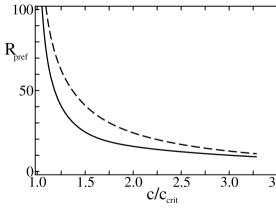
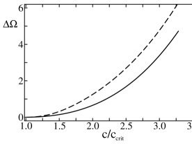
Figure 8: Preferential radius (in nm) and corresponding excess free energy density relative to the planar state (in units of $k_{\rm B}T$/(10 nm)³). The solid line corresponds to droplets containing low molecular mass polymer surrounded by a continuous phase consisting of the high molecular mass polymers. The dashed line is the reversed situation. In this example $\alpha=$ 8.

The preferential radius and the corresponding free energy are shown as a function of concentration in Figure 8. The preferential size of the (metastable) droplets is in the range of tenths of nanometers with the corresponding excess free energy of the polymer system of the order of a few $k_{\rm B}T$ per volume of (10 nm)³.

4 Summary

The interfacial tension between coexisting incompatible polymer solutions is calculated as a function of concentration for different degrees of polymerization and Kuhn segment lengths. This is done using the blob model for semi-dilute polymer solutions. It turns out that, when the degree of polymerization or the Kuhn length of the incompatible polymers differs, the interfacial tension is lowest when the interface has a certain preferential curvature. As a consequence, droplets of low molecular mass phase surrounded by a high molecular mass bulk phase may have an energy which is lower than that of the reversed situation. The preferential size was found to be of the order of tens of nanometers, and therefore observable by light scattering.

Appendix A Original analysis by Broseta

In this Appendix, we follow the analysis by Broseta et al. [13, 14, 15] of the profile of a planar interface between two coexistent polymer phases with solvent. The polymers have equal degrees of polymerization and are chemically identical with respect to the solvent. We start with expression for the free energy in Eq.(5) for a planar interface:

$$\frac{F[\phi,c]}{A\,k_{\rm B}T} = \int\limits_{-\infty}^{\infty}\!\!\!dz\left[\frac{\phi}{N_{b}\,\xi^{3}}\,\ln(\phi)+\frac{(1-\phi)}{N_{b}\,\xi^{3}}\,\ln(1-\phi)+\frac{u}{\xi^{3}}\,\phi\,(1-\phi)\right.$$ (38)

$$\left.+\frac{K}{\xi^{3}}+\frac{\phi^{\prime}(z)^{2}}{24\,\xi\,\phi}+\frac{\phi^{\prime}(z)^{2}}{24\,\xi\,(1-\phi)}+\frac{c^{\prime}(z)^{2}}{24\,\xi\,c^{2}}\right]\,.$$

Broseta et al. [14] continue by defining the dimensionless $\eta(z)$ and $\varepsilon(z)$ as:

$$\phi(z)\equiv\frac{1+\eta(z)}{2}\hskip 25.0pt{\rm and}\hskip 25.0ptc(z)\equiv c+\bar{u}\,c\,\varepsilon(z)\,.$$ (39)

The free energy per unit area then becomes

$$\frac{F[\eta,\varepsilon]}{A\,k_{\rm B}T} = \int\limits_{-\infty}^{\infty}\!\!\!dz\left[\frac{(1+\eta)}{2N_{b}\,\xi^{3}}\,\ln(1+\eta)+\frac{(1-\eta)}{2N_{b}\,\xi^{3}}\,\ln(1-\eta)+\frac{u}{4\,\xi^{3}}\,(1-\eta^{2})\right.$$ (40)

$$\left.+\frac{K}{\xi^{3}}+\frac{\eta^{\prime}(z)^{2}}{24\,\xi\,(1-\eta^{2})}+\frac{\bar{u}^{2}}{24\,\xi}\frac{\varepsilon^{\prime}(z)^{2}}{(1+\bar{u}\varepsilon)^{2}}\right]\,.$$

Next, an expansion is made by Broseta et al. [14] assuming that $\varepsilon(z)$ is small everywhere. One then has:

$$\frac{1}{N_{b}\,\xi^{3}} = \frac{1}{\bar{N}_{b}\,\bar{\xi}^{3}}(1+\bar{u}\varepsilon)\,,$$

$$\frac{1}{\xi^{3}} = \frac{1}{\bar{\xi}^{3}}(1+\frac{3\nu}{(3\nu-1)}\,\bar{u}\varepsilon+\frac{3\nu}{2\,(3\nu-1)^{2}}\,(\bar{u}\varepsilon)^{2}+\ldots)\,,$$

$$\frac{u}{\xi^{3}} = \frac{\bar{u}}{\bar{\xi}^{3}}(1+\frac{(3\nu+\chi)}{(3\nu-1)}\,\bar{u}\varepsilon+\ldots)\,.$$ (41)

To second order in $\varepsilon$, we then have for the free energy

$$\frac{F[\eta,\varepsilon]}{A\,k_{\rm B}T} = \frac{\bar{u}}{\bar{\xi}^{3}}\int\limits_{-\infty}^{\infty}\!\!\!dz\left[\frac{(1+\eta)}{2\omega}\,\ln(1+\eta)+\frac{(1-\eta)}{2\omega}\,\ln(1-\eta)-\frac{\eta^{2}}{4}+\frac{\bar{\xi}^{2}\,\eta^{\prime}(z)^{2}}{24\,\bar{u}\,(1-\eta^{2})}\right.$$ (42)

$$\left.+\frac{(1+\eta)}{2\omega}\,\ln(1+\eta)\,\bar{u}\,\varepsilon+\frac{(1-\eta)}{2\omega}\,\ln(1-\eta)\,\bar{u}\,\varepsilon-\frac{(3\nu+\chi)}{4\,(3\nu-1)}\,\eta^{2}\,\bar{u}\,\varepsilon\right.$$

$$\left.+\frac{3\nu\,K}{2\,(3\nu-1)^{2}}\,\bar{u}\,\varepsilon^{2}+\frac{\bar{\xi}^{2}}{24}\,\bar{u}\,\varepsilon^{\prime}(z)^{2}\right]\,,$$

where we have defined $\omega\!=\!\bar{N}_{b}\,\bar{u}$ [14] and omitted constants and terms proportional to a constant times $\varepsilon$. These are adsorbed in a constant bulk pressure $\tilde{p}$ and chemical potentials $\mu_{\eta}$ and $\mu_{\varepsilon}$. As a final step, we introduce $x\!\equiv\!z/D_{\infty}$, with $D_{\infty}\!\equiv\!\bar{\xi}/(6\bar{u})^{\frac{1}{2}}$ and the excess grand free energy due to the interface becomes:

$$\frac{\Omega[\eta,\varepsilon]}{A\,k_{\rm B}T} = \frac{(\bar{u}/6)^{\frac{1}{2}}}{\bar{\xi}^{2}}\int\limits_{-\infty}^{\infty}\!\!\!dx\left[\frac{(1+\eta)}{2\omega}\,\ln(1+\eta)+\frac{(1-\eta)}{2\omega}\,\ln(1-\eta)-\frac{\eta^{2}}{4}+\frac{\eta^{\prime}(x)^{2}}{4\,(1-\eta^{2})}\right.$$ (43)

$$\left.+\frac{(1+\eta)}{2\omega}\,\ln(1+\eta)\,\bar{u}\,\varepsilon+\frac{(1-\eta)}{2\omega}\,\ln(1-\eta)\,\bar{u}\,\varepsilon-\frac{(3\nu+\chi)}{4\,(3\nu-1)}\,\eta^{2}\,\bar{u}\,\varepsilon\right.$$

$$\left.+\frac{3\nu\,K}{2\,(3\nu-1)^{2}}\,\bar{u}\,\varepsilon^{2}+\frac{\bar{u}^{2}}{4}\,\varepsilon^{\prime}(x)^{2}-\mu_{\eta}\,\eta-\mu_{\varepsilon}\,\bar{u}\,\varepsilon+\tilde{p}\,\right]\,.$$

If we compare the expression above to (A10)-(12) in Broseta et al. [14], we see that the prefactor of $\varepsilon^{\prime}(x)^{2}$ should read $\bar{u}^{2}$ and not $\bar{u}$.

The above free energy is minimized in two steps. First, the profile $\eta_{0}(x)$ is determined assuming that $\varepsilon(x)\!=\!0$. One finds that the bulk value $\bar{\eta}$ ($\eta_{\ell}\!=\!\bar{\eta}$ and $\eta_{v}\!=\!-\bar{\eta}$) is determined by ($\mu_{\eta}\!=\!0$ by symmetry):

$$\frac{1}{\omega}\ln\left(\frac{1+\bar{\eta}}{1-\bar{\eta}}\right)-\bar{\eta}=0\,,$$ (44)

which has solutions for $\omega\!>\!\omega_{c}\!=\!2$ ($\bar{\eta}_{c}\!=\!0$). The profile $\eta_{0}(x)$ is determined by solving:

$$\frac{\eta_{0}^{\prime}(x)^{2}}{4\,(1-\eta_{0}^{2})}=\frac{(1+\eta_{0})}{2\omega}\,\ln(1+\eta_{0})+\frac{(1-\eta_{0})}{2\omega}\,\ln(1-\eta_{0})-\frac{\eta_{0}^{2}}{4}+\tilde{p}\,.$$ (45)

Second, using $\eta_{0}(x)$, the profile $\varepsilon_{0}(x)$ is determined. In the bulk $\bar{\varepsilon}\!=\!0$ which leads to the following expression for $\mu_{\varepsilon}$:

$$\mu_{\varepsilon}=\frac{(1+\bar{\eta})}{2\omega}\,\ln(1+\bar{\eta})+\frac{(1-\bar{\eta})}{2\omega}\,\ln(1-\bar{\eta})-\frac{3\nu+\chi}{4\,(3\nu-1)}\,\bar{\eta}^{2}\,.$$ (46)

The profile $\varepsilon_{0}(x)$ is determined by solving:

$$\frac{\bar{u}}{2}\,\varepsilon_{0}^{\prime\prime}(x) = \frac{(1+\eta_{0})}{2\omega}\,\ln(1+\eta_{0})+\frac{(1-\eta_{0})}{2\omega}\,\ln(1-\eta_{0})$$ (47)

$$+\frac{3\nu\,K}{(3\nu-1)^{2}}\,\varepsilon_{0}-\frac{(3\nu+\chi)}{4\,(3\nu-1)}\,\eta_{0}^{2}-\mu_{\varepsilon}\,.$$

Again, comparing with (18) in Broseta et al. [14], we see that the additional factor of $\bar{u}$ in the expression for the free energy in Eq.(43) leads to the presence of a factor $\bar{u}$ in front of $\varepsilon_{0}^{\prime\prime}(x)$.

With the help of these two profiles, the surface tension can then be calculated as:

$$\frac{\sigma\,\bar{\xi}^{2}}{k_{\rm B}T\,(\bar{u}/6)^{\frac{1}{2}}}=1-\Delta_{1}-\bar{u}\Delta_{2}\,.$$ (48)

with

$$\Delta_{1} = 1-2\int\limits_{0}^{\bar{\eta}}\!\!d\eta\left[\frac{(1+\eta)}{2\omega}\,\ln(1+\eta)+\frac{(1-\eta)}{2\omega}\,\ln(1-\eta)-\frac{\eta^{2}}{4}\right]^{\frac{1}{2}}(1-\eta^{2})^{-\frac{1}{2}}\,,$$

$$\Delta_{2} = \int\limits_{-\infty}^{\infty}\!\!\!dx\left[\frac{-\eta_{0}^{\prime}(x)^{2}}{8\,(1-\eta_{0}^{2})}+\frac{(1+\chi)}{8\,(3\nu-1)}\,(\eta_{0}^{2}-\bar{\eta}^{2})\right]\varepsilon_{0}(x)\,.$$ (49)

One sees that $\Delta_{1}$ is straightforwardly calculated from the above integral, but that for the calculations of $\Delta_{2}$ one needs to determine both density profiles $\eta_{0}(x)$ and $\varepsilon(x)$. The expression for $\Delta_{2}$ also differs from the one given in (29) in Broseta et al. [14].

References

- [1] Bergfeldt, K.; Piculell, L.; Linse, P. J. Phys. Chem. 1996, 100, 3680.
- [2] Tolstoguzov, V. Biotechnology Advances 2006, 24, 626.
- [3] Aarts, D.G.A.L.; van der Wiel, J.H.; Lekkerkerker, H.N.W. J. Phys.: Condens. Matt. 2003, 15, 245.
- [4] Ryden, J.; Albertsson, P.-A. J. of Coll. Interface Sci. 1971, 37, 219.
- [5] de Hoog, E.H.A.; Lekkerkerker, H.N.W. J. Phys. Chem. B 1999, 103, 5274.
- [6] Scholten, E.; Visser, J.E.; Sagis, L.M.C.; van der Linden, E. Langmuir 2004, 20, 2292.
- [7] Scholten, E.; Tuinier, R.; Tromp, R.H.; Lekkerkerker, H.N.W. Langmuir 2002, 18, 2234.
- [8] Simeone, M.; Alfani, A.; Guido, S. Food Hydrocolloids 2004, 18, 463.
- [9] van Puyvelde, P; Antonov, Y.A.; Moldenaers, P. Food Hydrocolloids 2002, 16, 395.
- [10] Antonov, Y.A.; van Puyvelde, P.; Moldenaers, P. International Journal of Biological Macromolecules 2004, 34, 29.
- [11] Mitani, S.; Sakai, K. Phys. Rev E. 2002, 66, 031604.
- [12] de Gennes, P.G. Scaling Concepts in Polymer Physics; Cornell University Press: Ithaca, 1979.
- [13] Broseta, D.; Leibler, L.; Lapp, A. Europhys. Lett. 1986, 2, 733.
- [14] Broseta, D.; Leibler, L.; Kaddour, O.; Strazielle, C. J. Chem. Phys. 1987, 87, 7248.
- [15] Broseta, D.; Leibler, L.; Joanny, J.-F. Macromolecules 1987, 20, 1935.
- [16] Tromp, R.H, Chapter 9 in Structure and Functional Properties of Colloidal Systems, Surfactant Science Series 146, Ed. Hidalgo-Alvarez, CRC Press: Boca Raton, 2010.
- [17] Flory, P.F. Principles of Polymer Chemistry; Cornell University Press: Ithaca, 1953.
- [18] Lapp A.; Picot C.; Strazielle, C. J. Phys. Lett. 1985, 46, L1031.
- [19] R.C. Tolman, J. Chem. Phys. 17, 333 (1949).
- [20] E.M. Blokhuis and D. Bedeaux, J. Chem. Phys. 97, 3576 (1992).
- [21] Helfrich, W. Z. Naturforsch. C 1973, 28, 693.
- [22] Blokhuis, E.M.; Bedeaux, D. Mol. Phys. 1993, 80, 705.
- [23] Blokhuis, E.M.; Kuipers, J. J. Chem. Phys. 2006, 124, 074701.
- [24] E.M. Blokhuis and A.E. van Giessen, arXiv:cond-mat/13046557.