Kondo screening by the surface modes of a strong topological insulator

Abstract

We consider a magnetic impurity deposited on the surface of a strong topological insulator and interacting with the surface modes by a Kondo exchange interaction. Taking into account the warping of the Fermi line of the surface modes, we derive a mapping to an effective one dimensional model and show that the impurity is fully screened by the surface electrons except when the Fermi level lies exactly at the Dirac point. Using an Abrikosov fermion mean-field theory, we calculate the shape of the electronic density Friedel oscillation resulting from the presence of the Kondo screening cloud. We analyze quantitatively the observability of a six-fold symmetry in the Friedel oscillations for two prototype compounds: Bi₂Se₃ and Bi₂Te₃.

I Introduction

Topological insulators are a new class of materials, with an insulating bulk and a conducting surface.HasanMoore2010 ; HasanKane2010 ; QiZhang2010 . The existence of four topological invariants guarantees the stability of these surface states against perturbations.Fu2007 ; moore2007 ; roy2009 Furthermore, the topological invariants permit to distinguish two types of topological insulators, the weak topological insulators and the strong topological insulators. In a strong topological insulator, the surface modes at low energy form an odd number of Dirac cones. This is to be contrasted with a strictly two-dimensional conductor such as graphenecastroneto2009 , where the Nielsen-Ninomiya theoremNielsen1981 only permits an even number of Dirac cones: the presence of the gapped bulk is crucial to the formation of an odd number of Dirac cones. Experimentally, the material $\mathrm{Bi_{x}Sb_{1-x}}$ is a strong topological insulator with three Dirac coneshsieh2008 while $\mathrm{Bi_{2}Se_{3}}$, $\mathrm{Bi_{2}Te_{3}}$ and $\mathrm{Sb_{2}Te_{3}}$, are strong topological insulators with a single Dirac cone.zhang2009 ; chen2009 In the case of $\mathrm{Bi_{2}Te_{3}}$, a significant hexagonal Fermi line warping is present.chen2009 More recent examples of topological insulator materials are $\mathrm{TlBiSe_{2}}$sato2010 , strained HgTebruene2011 ; bouvier2011 , $\mathrm{Bi_{2}Te_{1.6}S_{1.4}}$ji2012 $\mathrm{PbBi_{2}Te_{4}}$kuroda2012 , $\mathrm{Pb}({\mathrm{Bi}}_{1-x}{\mathrm{Sb}}_{x}{)}_{2}{\mathrm{Te}}_{4}$souma2012 , $\mathrm{Bi_{2}Se_{2}Te}$, $\mathrm{Bi_{2}Te_{2}Se}$, and $\mathrm{GeBi_{2}Te_{4}}$.neupane2012 It has also recently been proposed on the basis of band structure calculations that the ternary compound LiAuSezhang2011 and the cerium filled skutteruditesyan2012 $\mathrm{CeOs_{4}As_{12}}$ and $\mathrm{CeOs_{4}As_{12}}$, could be topological insulators. A recent review of known topological insulators can be found in Ref. yan2012a, . In all these systems, a strong spin-orbit coupling is present, and in the surface states the helicity, i.e., the sign of the spin projection of the quasiparticle spin on the quasi-momentum is fixed. An interesting theoretical question is then whether the Kondo effectKondo1964 ; nozieres_shift ; Wilson1975 ; andrei_kondo_review in the surface modes is affected by a fixed helicity. In particular, one would like to know whether a conventional Kondo effect takes place, or whether the fixed helicity constraint gives rise to unconventional Kondo fixed points. In the case of two-dimensional topological insulatorsWu2006 , the question was addressedtanaka2011 , and it was shown that a conventional Kondo effect would take place, leading to a suppression of the backscattering of the edge states by magnetic impurities. In the case of a three-dimensional topological insulator, the Anderson model was considered both in the absenceFeng2009 ; zitko2010 ; tran2010 and in the presencemitchell2012 of Fermi surface warping. Within a variational trial wavefunction method, it was found that the local moment would be fully quenched, but correlations would exist between the conduction electron spin and the spin of the local impurity.Feng2009 Analogous results were obtained in a two-dimensional electron gas with Rashba and Dresselhaus spin-orbit couplings.feng2011 In the case of a pure Dirac spectrum, a mapping on the one-dimensional Anderson model with a pseudogap in the hybridization function was obtained.zitko2010 ; tran2010 It was concluded that away from the Dirac point the Kondo effect would take place, and the impurity would be fully screened, while at the Dirac point, the local moment would decouple.zitko2010 The local density of states (LDOS), the local spin density of states (LSDOS) and the Friedel oscillations were also investigatedtran2010 within a U(1) slave-bosonhewson1997 mean-field theory. In Ref.mitchell2012, , the Anderson model in a topological insulator with a Fermi surface warping was considered using the numerical renormalization group and the behavior of the LDOS was obtained. Experimentally, magnetic impurities such as manganesenoh2011 , nickel, ironwray2011 ; scholz2012 ; shelford2012 , cobaltye2012 ; shelford2012 and gadoliniumvalla2012 have been deposited on the surface of topological insulators. It was found that the surface states were remarkably insensitive to the presence of both magnetic and nonmagnetic impuritiesnoh2011 ; valla2012 . While the first result can be understood as a consequence of the suppression of backscattering, the second result is more surprising since magnetic impurities permit backscattering by flipping the electron spin.

Besides this single impurity behavior, it has been suggested theoretically that in a Kondo lattice at electronic half-filling, the Kondo interaction could help the formation of a topological insulator.dzero2012 ; dzero2012a ; tran2012 ; zhang2012 There are indeed recent experimental indications that the Kondo insulatorzhang_smb6_2012 ; botimer2012 $\mathrm{SmB_{6}}$ could be a topological insulator. This also lends support to the hypothesis that Kondo screening of magnetic impurities is compatible with the helical character of the surface states. An important technique to probe conducting surfaces is Scanning Tunneling Microscopy (STM).binnig1982 ; binnig1987 This is particularly interesting in relation to the Kondo effect since STM measurements of the LDOS around a Kondo impurity located on the surface of a metal have already been performedmadhavan1998 ; madhavan2001 ; knorr2002 ; wahl2005 ; ysfu2007 , and the influence of the Kondo resonance on the LDOS has been studied theoreticallyujsaghy2000 . Since the surface of a topological insulator is conducting, it can be probed by STM.roushan2009 ; beidenkopf2011 ; alpichshev2011 ; alpichshev2012 ; cheng2012 ; teague2012 ; zhang2013 The existing predictions for the LDOS caused by a Kondo impuritymitchell2012 could thus be tested in that manner. Moreover, following the proposal of Ref. affleck2008, , integrating the measured LDOS would permit the measurement of the Friedel oscillations of the electron density induced by the Kondo screening cloud around the magnetic impurity.

In the present paper, we want to further analyze the Kondo effect of a magnetic impurity at the surface of a strong topological insulator with warping. In the first part, we reduce the Kondo Hamiltonian to a one-dimensional model which can be treated by integrability techniques. We find that a conventional Kondo effect is obtained, with the impurity screened by the surface modes unless the Fermi level is right at the Dirac point, in which case, because of the vanishing density of states, the impurity remains unscreened for weak Kondo coupling. In the second part, we calculate within an Abrikosov fermion mean-field theoryabrikosov_kondo the Friedel oscillationsaffleck2008 resulting from the existence of the Kondo screening cloud. For weak Fermi surface warping, we derive a perturbative expression of the density Friedel oscillations. In the third part we discuss the observability in STM measurements of the Friedel oscillations of electron densityaffleck2008 around an impurity in the specific cases of two prototype compounds: $\mathrm{Bi_{2}Se_{3}}$ and $\mathrm{Bi_{2}Te_{3}}$.

II Mapping to a one-dimensional model

The free electrons Hamiltonian of the surface modes of a strong topological insulator with warping reads:

$$H_{0}\equiv\sum_{\mathbf{k},\alpha,\beta}c^{\dagger}_{\mathbf{k},\alpha}[-iv_{F}\mathrm{\hat{z}}\cdot(\boldsymbol{\sigma}_{\alpha\beta}\times\mathbf{k})+\frac{\lambda}{2}[(k_{x}+ik_{y})^{3}+(k_{x}-ik_{y})^{3}]\sigma^{z}-\mu\delta_{\alpha\beta}]c_{\mathbf{k},\beta} \equiv \sum_{\mathbf{k},\alpha,\beta}c^{\dagger}_{\mathbf{k},\alpha}\mathcal{H}^{0}_{\alpha\beta}(\mathbf{k})c_{\mathbf{k},\beta}~{},$$ (1)

where $c_{\mathbf{k},\alpha}$ annihilates a fermion of momentum $\mathbf{k}$ and spin $\alpha$, $\hat{z}$ is the normal to surface of the topological insulator, $\boldsymbol{\sigma}=(\sigma^{x},\sigma^{y},\sigma^{z})$ denotes the Pauli matrices, $v_{F}$ is the Fermi velocity, $\lambda$ is the warping, and $\mu$ the chemical potential. In the case of $\mathrm{Bi_{2}Se_{3}}$, one haskuroda2010 $v_{F}=3.55$ eVÅ  and $\lambda=128$ eVų. For $\mathrm{Bi_{2}Te_{3}}$, chen2009 ; an2012 one has $v_{F}=2.55$ eVÅ and $\lambda=250$ eVÅ. In the following we will study the effects induced by the presence of a magnetic quantum impurity. We take the position of the impurity as the origin of our coordinates so that the Kondo Hamiltonian describing the surface modes and their interaction with the impurity reads:

$$H = H_{0}+H_{K}\equiv H_{0}+\frac{J_{K}}{L^{2}}\sum_{\mathbf{k},\mathbf{k^{\prime}},\alpha,\beta}\mathbf{S}\cdot c^{\dagger}_{\mathbf{k},\alpha}\boldsymbol{\sigma}_{\alpha\beta}c_{\mathbf{k^{\prime}},\beta}~{},$$ (2)

where $J_{K}$ is the Kondo interaction, $L$ the linear dimension of the (square) surface, $\mathbf{S}$ the impurity spin.

II.1 Eigenstates of the free Hamiltonian

In the present section, we briefly review the eigenstates of the free electrons Hamiltonian (1). We will use a spinor notation to represent the Fermion annihilation and creation operators:

$$\Psi(\mathbf{r})=\left(\begin{array}[]{c}\psi_{\uparrow}(\mathbf{r})\\ \psi_{\downarrow}(\mathbf{r})\end{array}\right)=\sum_{s=\pm}\int\frac{d^{2}\mathbf{k}}{(2\pi)^{2}}\psi_{\mathbf{k}}^{s}(\mathbf{r})c_{s}(\mathbf{k}),$$ (3)

where the spinors $\psi_{\mathbf{k}}^{s}(\mathbf{r})$ are eigenstates of the first quantized Hamiltonian and $\{c_{s}(\mathbf{k}),c_{s^{\prime}}(\mathbf{k^{\prime}})\}=(2\pi)^{2}\delta_{s,s^{\prime}}\delta(\mathbf{k}-\mathbf{k^{\prime}})$. Introducing the polar coordinates $\mathbf{k}\equiv(k,\phi)$ and $\mathbf{r}\equiv(r,\theta)$ the spinors have the explicit form:

$$\psi_{k,\phi}^{s}(r,\theta)=\left(\begin{array}[]{c}A_{s}\\ -iB_{s}e^{i\phi}\end{array}\right)e^{ikr\cos(\theta-\phi)},$$ (4)

where $|A_{s}|^{2}+|B_{s}|^{2}=1$ and

$$\frac{A_{s}+iB_{s}}{A_{s}-iB_{s}}=s\frac{\lambda k^{3}\cos 3\theta+iv_{F}k}{\sqrt{v_{F}^{2}k^{2}+\lambda^{2}k^{6}\cos^{2}3\theta}}~{}.$$ (5)

We note that $A_{s}$ and $B_{s}$ are periodic functions of $\theta$ of period $\frac{2\pi}{3}$. In the rotationally invariant case, i.e., without the warping term ($\lambda=0)$, the eigenstates of the Hamiltonian are rewritten as angular momentum eigenstates, and only the s-wave channelzitko2010 ; tran2010 is found to contribute to the Kondo interaction. In the case with warping ($\lambda\neq 0$), there is only a discrete rotational symmetry, and instead of representations of $O(2)$ the eigenstates have to be expressed as representations of the discrete group $Z_{3}$:

$$\psi^{s}_{k,\phi,\ell}(\mathbf{r}) = \frac{1}{\sqrt{3}}\sum_{n=0,1,2}e^{i\frac{2\pi}{3}\ell n}\psi^{s}_{k,\phi+\frac{2n\pi}{3}}(\mathbf{r}),$$ (6)

with the restriction $|\phi|<\pi/3$ and $\ell=0,1,2$ labels the representation. With full rotational symmetry, $\ell$ would be the angular momentum. Because of the 3-fold symmetry of the warping term, the states having a difference of angular momentum equal to a multiple of 3 are hybridized together, and the angular momentum $\ell$ is defined only modulo 3. In that basis, the spinor (3) reads:

$$\Psi(\mathbf{r})=\sum_{\ell,s=\pm}\int\frac{d^{2}\mathbf{k}}{(2\pi)^{2}}\psi^{s}_{\mathbf{k},\ell}(\mathbf{r})c_{\ell,s}(\mathbf{k})~{}.$$ (7)

Since $\psi^{s}_{k,\phi,1}(0,\theta)=0$, only the $\ell=0,2$ modes interact with the magnetic impurity:

$$\Psi(\mathbf{0})=\sqrt{3}\int\frac{d^{2}\mathbf{k}}{(2\pi)^{2}}\left(\begin{array}[]{c}Ac_{0,+}(\mathbf{k})-Bc_{0,-}(\mathbf{k})\\ -iBc_{2,+}(\mathbf{k})-iAc_{2,-}(\mathbf{k})\end{array}\right)~{},$$ (8)

and the Kondo Hamiltonian is rewritten as:

$$H = \sum_{\ell,s}\int\frac{d^{2}\mathbf{k}}{(2\pi)^{2}}(sE(\mathbf{k})-\mu)c^{\dagger}_{\ell,s}(\mathbf{k})c_{\ell,s}(\mathbf{k})+J_{K}\mathbf{S}\cdot\Psi^{\dagger}(\mathbf{0})\boldsymbol{\sigma}\Psi(\mathbf{0})~{},$$ (9)

with

$$E(\mathbf{k})\equiv\sqrt{v_{F}^{2}k^{2}+\lambda^{2}k^{6}\cos^{2}(3\phi)}~{}.$$ (10)

The Hamiltonian (9) can be further reduced by turning the integration variable $\mathbf{k}$ to a system of curvilinear coordinates $(E,\kappa_{\perp})$, where $E$ is the energy of the eigenstate, and $\kappa_{\perp}$ is the curvilinear coordinate along the line of constant energy. Introducing the new operators:

$$a_{\ell,s}(E,\kappa_{\perp})=\frac{c_{\ell,s}(\mathbf{k})}{\sqrt{||\nabla_{\mathbf{k}}E(\mathbf{k})||}}~{},$$ (11)

with anticommutation relations $\{a_{\ell,s}(E,\kappa_{\perp}),a^{\dagger}_{\ell,s}(E^{\prime},\kappa^{\prime}_{\perp})\}=(2\pi)^{2}\delta(E-E^{\prime})\delta(\kappa_{\perp}-\kappa^{\prime}_{\perp})$, the free electrons part of the Hamiltonian (9) can be rewritten:

$$H_{0}=\sum_{\ell,s}\int\frac{dEd\kappa_{\perp}}{(2\pi)^{2}}(sE-\mu)a^{\dagger}_{\ell,s}(E,\kappa_{\perp})a_{\ell,s}(E,\kappa_{\perp})~{}.$$ (12)

Introducing the density of states:

$$\rho_{0}(E)\equiv\int\frac{d\kappa_{\perp}}{4\pi^{2}||\nabla_{\mathbf{k}}E(\mathbf{k})||}~{},$$ (13)

and the operators:

$$a_{\uparrow,+}(E)=\sqrt{3}\int d\kappa_{\perp}\frac{A(E,\kappa_{\perp})a_{0,+}(E,\kappa_{\perp})}{\sqrt{2\pi^{2}\rho_{0}(E)||\nabla_{\mathbf{k}}E(\mathbf{k})||}}~{},$$ (14)

$$a_{\uparrow,-}(E)=\sqrt{3}\int d\kappa_{\perp}\frac{B(E,\kappa_{\perp})a_{0,-}(E,\kappa_{\perp})}{\sqrt{2\pi^{2}\rho_{0}(E)||\nabla_{\mathbf{k}}E(\mathbf{k})||}}~{},$$ (15)

$$a_{\downarrow,+}(E)=\sqrt{3}\int d\kappa_{\perp}\frac{B(E,\kappa_{\perp})a_{2,+}(E,\kappa_{\perp})}{\sqrt{2\pi^{2}\rho_{0}(E)||\nabla_{\mathbf{k}}E(\mathbf{k})||}}~{},$$ (16)

$$a_{\downarrow,-}(E)=\sqrt{3}\int d\kappa_{\perp}\frac{A(E,\kappa_{\perp})a_{2,-}(E,\kappa_{\perp})}{\sqrt{2\pi^{2}\rho_{0}(E)||\nabla_{\mathbf{k}}E(\mathbf{k})||}}~{},$$ (17)

with anticommutators $\{a_{\alpha,s}(E),a^{\dagger}_{\alpha^{\prime},s^{\prime}}(E^{\prime})\}=(2\pi)^{2}\delta(E-E^{\prime})\delta_{ss^{\prime}}\delta_{\alpha\alpha^{\prime}}$ we can define:

$$a_{\alpha}(E)=(-i)^{1/2-\alpha}\sum_{s=\pm}\Theta(sE)s^{1/2+\alpha}a_{\alpha,s}(|E|)~{},$$ (18)

$$\psi_{\alpha}(0)=\int_{-\infty}^{\infty}\frac{dE\sqrt{\rho_{0}(|E|)}}{\pi\sqrt{8}}a_{\alpha}(E)~{},$$ (19)

where $\Theta$ denotes the Heaviside function. In terms of these operators, the Kondo Hamiltonian (9) reads:

$$H=J_{K}\mathbf{S}\cdot\Psi^{\dagger}(\mathbf{0})\boldsymbol{\sigma}\Psi(\mathbf{0})+\int_{-\infty}^{+\infty}\frac{dE}{(2\pi)^{2}}\sum_{\alpha}(E-\mu)a^{\dagger}_{\alpha}(E)a_{\alpha}(E)+\ldots~{},$$ (20)

where $\ldots$ stands for the modes of the free electrons Hamiltonian $H_{0}$ that do not couple to the impurity. Away from the Dirac point, the density of states $\rho_{0}(E)$ can be approximated by the density of states at the Fermi level $\rho_{0}(\mu)$, and the usual single channel Kondo problem is obtained. For a spin-1/2 impurity, The Kondo temperature can be obtained from the Bethe Ansatz solution asandrei_trieste93 :

$$T_{K}=De^{\gamma_{E}-1/4}\exp\left(\frac{-1}{J_{K}\rho_{0}(\mu)}\right),$$ (21)

where $\gamma_{E}\simeq 0.577$ is the Euler-Mascheroni constant and $D$ is a symmetric cutoff around the Fermi energy. The density of states $\rho_{0}(E)$ can be expressed in terms of elliptic integralsadroguer2012 , so the full dependence of the Kondo temperature on the chemical potential is known up to the prefactor $D$. Since the Bethe Ansatz solution of the Kondo problemandrei_trieste93 requires a constant density of states, $D$ represents as the energy scale away from the Fermi energy for which the density of states starts to deviate significantly from the density of states at the Fermi energy. For small warping $\lambda$ or not too far from the Dirac point, the density of states is a linear function of energy, and $D\simeq\mu$, so the dependence of $D$ on $E$ is only a subdominant contribution. Close to the Dirac point, $\mu\to 0$, the density of states $\rho_{0}(\mu)\sim|\mu|$. Because of such pseudogap, the Kondo temperature vanishesWithoff1990 . These results are in agreement with the ones derived in the framework of the Anderson modelzitko2010 ; tran2010 where Kondo screening was obtained only when the density of states at the Fermi level was non-vanishing. In the case of an impurity with spin $S>1/2$ Eq. (20) would give the underscreened single channel Kondo fixed point.

More generally, it can be established in any dimension $d$ that with any free Hamiltonian of the form:

$$H_{0}=\sum_{\alpha,\beta}c^{\dagger}_{k,\alpha}(\mu\delta_{\alpha\beta}+\boldsymbol{\epsilon}(\mathbf{k})\cdot\boldsymbol{\sigma}_{\alpha\beta})c_{k,\beta}~{},$$ (22)

having time reversal symmetry (i. e. $\boldsymbol{\epsilon}(-\mathbf{k})=-\boldsymbol{\epsilon}(\mathbf{k})$) only a conventional Kondo effect can be obtained. Indeed, if we write the partition function asanderson_kondo_2 :

$$Z=Z_{0}\left\langle T_{\tau}e^{-J_{K}\int_{0}^{\beta}d\tau\mathbf{S}(\tau)\cdot\psi^{\dagger}_{\alpha}(0,\tau)\boldsymbol{\sigma}_{\alpha\beta}\psi_{\beta}(0,\tau)}\right\rangle_{H_{0}}~{},$$ (23)

with $Z_{0}\equiv Tr~{}e^{-\beta H_{0}}$, and expand in powers of $J_{K}$, the series will depend on:

$$G_{\alpha\beta}(0,\tau)=\frac{1}{\beta}\sum_{i\nu_{n}}\int\frac{d^{d}\mathbf{k}}{(2\pi)^{d}}\frac{(i\nu_{n}+\mu)\delta_{\alpha\beta}+\boldsymbol{\epsilon}(\mathbf{k})\cdot\boldsymbol{\sigma}_{\alpha\beta}}{(i\nu_{n}+\mu)^{2}-\|\boldsymbol{\epsilon}(\mathbf{k})\|^{2}}e^{i\nu_{n}\tau}~{},$$ (24)

but since $\boldsymbol{\epsilon}(\mathbf{k})$ is odd, introducing the density of states $\rho_{0}(E)=\int\delta(E-\|\boldsymbol{\epsilon}(\mathbf{k})\|)d^{d}\mathbf{k}/(2\pi)^{d}$ we can write:

$$G_{\alpha\beta}(0,\tau)=\frac{1}{2\beta}\sum_{i\nu_{n}}\int\frac{\rho_{0}(|E|)\delta_{\alpha\beta}}{i\nu_{n}+\mu-E}dE~{},$$ (25)

showing that the partition function is the same as the one of a system without spin-orbit coupling having the same density of states $\rho_{0}$ as the Hamiltonian (22). As a result, a conventional Kondo effect is realized every time the density of states at the Fermi level is nonzeroanderson_kondo_2 . As a consequence, the dispersion and the Kondo self-energy are expected to remain spin-independent much beyond the mean-field approximation that we will consider in the following.

III Friedel oscillations and Abrikosov fermions mean-field theory

III.1 Mean-field theory

III.1.1 Abrikosov fermions and mean-field self-consistent relations

We have seen in Sec.II that even in the presence of warping, a magnetic impurity on the surface of a topological insulator is always screened provided the density of states at the Fermi level is nonzero. In such conditions, a Kondo screening cloudaffleck2008 is formed around the impurity, and Friedel oscillations are formed. We consider in the following the case of a fully screened $S=1/2$ impurity. Since we are dealing with a conventional Kondo fixed point, we can use the Abrikosov fermion representationabrikosov_kondo for the localized spin:

$$S^{+}=f^{\dagger}_{\uparrow}f_{\downarrow};~{}~{}S^{-}=f^{\dagger}_{\downarrow}f_{\uparrow};~{}~{}S^{z}=\frac{1}{2}(f^{\dagger}_{\uparrow}f_{\uparrow}-f^{\dagger}_{\downarrow}f_{\downarrow})~{},$$ (26)

with the constraint

$$1 = f^{\dagger}_{\uparrow}f_{\uparrow}+f^{\dagger}_{\downarrow}f_{\downarrow}~{},$$ (27)

to rewrite the Kondo interaction as a local fermion-fermion interaction:

$$H_{K}=J_{K}\mathbf{S}\cdot\Psi^{\dagger}(\mathbf{0})\boldsymbol{\sigma}\Psi(\mathbf{0})=\frac{J_{K}}{2}\left(\sum_{\alpha\beta}f^{\dagger}_{\alpha}f_{\beta}\psi^{\dagger}_{\beta}(0)\psi_{\alpha}(0)-\sum_{\alpha}\frac{\psi^{\dagger}_{\alpha}(0)\psi_{\alpha}(0)}{2}\right)~{},$$ (28)

where the two terms on the r.h.s. respectively correspond to the spin-flip and charge potential scattering processes of conduction electrons on the Kondo impurity. Hereafter we will concentrate on the spin-flip interaction term and we will neglect the charge potential scattering one. Adding a Lagrange multiplier $\mu_{f}(1-\sum_{\alpha}f^{\dagger}_{\alpha}f_{\alpha})$ to the full Kondo Hamiltonian $H_{0}+H_{K}$ to enforce the constraint (27), we decouple (28) by a mean-field approximation:

$$H_{MF} = H_{0}+\Delta\sum_{\alpha}(f^{\dagger}_{\alpha}\psi_{\alpha}(0)+\mathrm{H.c.})-\mu_{f}\sum_{\alpha}f^{\dagger}_{\alpha}f_{\alpha},$$ (29)

where the effective hybridization $\Delta$ and the Lagrange multiplier $\mu_{f}$ satisfy the self-consistent relations :

$$\Delta = \frac{J_{K}}{2}\sum_{\alpha}\langle\psi^{\dagger}_{\alpha}f_{\alpha}\rangle~{},$$ (30)

$$1 = \sum_{\alpha}\langle f^{\dagger}_{\alpha}f_{\alpha}\rangle~{},$$ (31)

where $\langle\cdots\rangle$ denotes the thermal average computed with the mean-field effective Hamiltonian (29). We introduce the Fourier decomposition:

$$\psi_{\alpha}(\mathbf{r})=\frac{1}{L}\sum_{\mathbf{k}}c_{\mathbf{k}\alpha}e^{i\mathbf{k}\cdot\mathbf{r}}~{},$$ (32)

where $L^{2}$ is the surface of the system. To solve the mean field equations, we introduce the Green’s functions

$$G_{\alpha\beta}^{cc}(\mathbf{k},\mathbf{k^{\prime}},\tau) = -\langle T_{\tau}c_{\mathbf{k}\alpha}(\tau)c_{\mathbf{k^{\prime}}\beta}^{\dagger}(0)\rangle~{},$$

$$G_{\alpha\beta}^{fc}(\mathbf{k^{\prime}},\tau) = -\langle T_{\tau}f_{\alpha}(\tau)c_{\mathbf{k^{\prime}}\beta}^{\dagger}(0)\rangle~{},$$

$$G_{\alpha\beta}^{cf}(\mathbf{k},\tau) = -\langle T_{\tau}c_{\mathbf{k}\alpha}(\tau)f^{\dagger}_{\alpha}(0)\rangle~{},$$

$$G_{\alpha\beta}^{ff}(\tau) = -\langle T_{\tau}f_{\alpha}(\tau)f_{\beta}^{\dagger}(0)\rangle~{}.$$ (33)

Using the equations of motion from the Hamiltonian (29) and a Fourier decomposition in Matsubara frequencies, the Green’s functions in (III.1.1) are expressed as:

$$G^{cc}(\mathbf{k},\mathbf{k^{\prime}},i\nu_{n}) = \delta_{\mathbf{k},\mathbf{k^{\prime}}}G_{0}(\mathbf{k},i\nu_{n})+\frac{|\Delta|^{2}}{L^{2}}G_{0}(\mathbf{k},i\nu_{n})G^{ff}(i\nu_{n})G_{0}(\mathbf{k^{\prime}},i\nu_{n})~{},$$ (34)

$$G^{fc}(\mathbf{k},i\nu_{n}) = -\frac{\Delta^{\star}}{L}G^{ff}(i\nu_{n})G_{0}(\mathbf{k},i\nu_{n})~{},$$ (35)

$$G^{cf}(\mathbf{k},i\nu_{n}) = -\frac{\Delta}{L}G_{0}(\mathbf{k},i\nu_{n})G^{ff}(i\nu_{n})~{},$$ (36)

$$G^{ff}(i\nu_{n}) = (i\nu_{n}+\mu_{f}-\Sigma(i\nu_{n}))^{-1},$$ (37)

with the free electrons Green function :

$$G_{0}(\mathbf{k},i\nu_{n}) \equiv (i\nu_{n}-{\cal H}^{0}(\mathbf{k}))^{-1}~{},$$ (38)

and the self-energy:

$$\Sigma(i\nu_{n})=|\Delta|^{2}\int\frac{d^{2}\mathbf{k}}{(2\pi)^{2}}G_{0}(\mathbf{k},i\nu_{n})~{}.$$ (39)

Hereafter, we introduce the non-interacting electronic density of states, $\rho_{0}(E)\equiv\int\delta(E-\epsilon_{\mathbf{k}})d^{2}\mathbf{k}/(2\pi)^{2}$, where $\epsilon_{\mathbf{k}}$ denotes the electronic eigenenergies. Remarking that ${\cal H}^{0}(\mathbf{k})$ has time reversal symmetry, and invoking a similar analysis as the one leading to Eq. (25), we find the following spin-independent expression for the self-energy:

$$\Sigma_{\alpha\beta}(z) \equiv \delta_{\alpha\beta}|\Delta|^{2}\int_{-\infty}^{\infty}dE\frac{\rho_{0}(E)}{z+\mu-E}~{}.$$ (40)

Introducing the real and imaginary parts of the self-energy, $\Sigma_{\alpha\beta}(E+i0^{+})=\delta_{\alpha\beta}[\Sigma^{\prime}(E)+i\Sigma^{\prime\prime}(E)]$, with

$$\Sigma^{\prime}(E) = |\Delta|^{2}\int_{-\infty}^{\infty}d\epsilon\rho_{0}(\epsilon)\mathrm{P.V.}\left(\frac{1}{E+\mu-\epsilon}\right)~{},$$ (41)

$$\Sigma^{\prime\prime}(E) = -\pi|\Delta|^{2}\rho_{0}(E+\mu)~{},$$ (42)

the self-consistency conditions (30) and (31) read:

$$|\Delta|^{2} = J_{K}\int_{-\infty}^{\infty}\frac{dE}{\pi}n_{F}(E)\frac{(E+\mu_{f})\Sigma^{\prime\prime}(E)}{[E+\mu_{f}-\Sigma^{\prime}(E)]^{2}+[\Sigma^{\prime\prime}(E)]^{2}}~{},$$ (43)

$$\frac{1}{2} = -\int_{-\infty}^{\infty}\frac{dE}{\pi}n_{F}(E)\frac{\Sigma^{\prime\prime}(E)}{[E+\mu_{f}-\Sigma^{\prime}(E)]^{2}+[\Sigma^{\prime\prime}(E)]^{2}}~{}.$$ (44)

III.1.2 Kondo temperature

On general grounds, the Kondo temperature $T_{K}$ indicates a crossover between the high temperature weakly coupled and the low temperature strongly coupled regimes. Indeed, the system at temperatures below $T_{K}$ is characterized by a magnetic confinement of the spin of the edge electronic states which screens the Kondo impurity hewson1997 . $T_{K}$ has been shown to be the unique energy scale that characterizes the universal physical properties of single impurity Kondo models at low temperature $T\ll T_{K}$. We will see later how this scaling property will become extremely useful for analyzing universal properties of the electronic density at very low temperature. But before, we derive here an expression of $T_{K}$. Within the mean-field approximation, the Kondo crossover turns to a transition at $T_{K}$ which corresponds to a continuous vanishing of the $f-c$ effective hybridization: $\Delta(T_{K})=0$. Invoking the self-consistent relations (43) and (44), we find (see appendix A.1) the following mean-field equation for $T_{K}$:

$$\mu_{f}=0~{},$$ (45)

and

$$\frac{2}{J_{K}}=P.V.\int_{-\infty}^{+\infty}dE\frac{n_{F}(E)}{E}\rho_{0}(\mu+E)~{},$$ (46)

which is equivalent to the Nagaoka-Suhl equation derived in Refs. nagaoka_resonance, and suhl_resonance, . Assuming an even free electrons density of state, $\rho_{0}(-E)=\rho_{0}(E)$, a general explicit expression of $T_{K}$ was derived in the weak Kondo coupling limitburdin2000 ; burdin2009

$$T_{K} = F_{K}e^{-1/J_{K}\rho_{0}(\mu)}~{},$$ (47)

with

$$F_{K} = \frac{2e^{\gamma_{E}}}{\pi}(D+\mu)\exp\left[-\int_{-D-\mu}^{0}\frac{dE}{E}\frac{\rho_{0}(\mu+E)-\rho_{0}(\mu)}{\rho_{0}(\mu)}\right]~{},$$ (48)

where $\gamma_{E}\simeq 0.577$ is the Euler-Mascheroni constant, and $D$ denotes the half-bandwidth of $\rho_{0}$. The mean-field expression (47) provides the usual non-analytic exponential term characterizing the $J_{K}-$dependence of the Kondo temperature at small Kondo coupling $J_{K}\rho_{0}(\mu)\ll 1$. The same exponential dependence also emerges from the mapping to the Bethe Ansatz solvable model (see Eq. 21). The prefactor $F_{K}$ does not depend on $J_{K}$ and is thus a pure characteristics of the non-interacting electronic system. Whatever the specific chemistry of the magnetic impurity is and whatever the microscopic details of its coupling with conduction electrons, the prefactor $F_{K}$ depends only on the energy structure of the non-interacting conduction electrons.

We find that $F_{K}\sim D$ if one assumes a constant density of states and a chemical potential close to the middle of the electronic energy band. The situation may become quantitatively different when the conduction electrons describe the surface modes of a topological insulator. Indeed, using the density of states $\rho(E)=|E|/(2\pi v_{F}^{2})$ that characterizes a surface mode without warping, we find for $\mu>0$:

$$T_{K}=\frac{2e^{\gamma_{E}-1}}{\pi}\frac{\mu^{2}}{D+\mu}\exp{\left(\frac{D}{\mu}-\frac{2\pi v_{F}^{2}}{J_{K}\mu}\right)}.$$ (49)

This small $J_{K}$ asymptotic expression becomes singular at the Dirac point $\mu=0$, where the density of states vanishes linearly. At the Dirac point, one has to start from the equation (46) for the Kondo temperature, which simplifies to:

$$\frac{1}{J_{K}} = \int_{0}^{D}\frac{dE}{2\pi v_{F}^{2}}\tanh\left(\frac{E}{2T_{K}}\right),$$ (50)

$$= \frac{T_{K}}{\pi v_{F}^{2}}\ln\left[\cosh\left(\frac{D}{2T_{K}}\right)\right],$$ (51)

where $D$ is a bandwidth cutoff. For $J_{K}<J_{K}^{c}\equiv\frac{2\pi v_{F}^{2}}{D}$, the Eq. (50) has no solution, in agreement with the results of Ref. Withoff1990, . For $J_{K}>J_{K}^{c}$, we find that:

$$T_{K}=\frac{D}{2\ln 2}\left(1-\frac{J_{K}^{c}}{J_{K}}\right),$$ (52)

indicating that regular Kondo effect can still be realized at the Dirac point, but with a Kondo temperature vanishing linearly with the Kondo interaction when $J_{K}\to J_{K}^{c}$, in agreement with the prediction of Ref. Withoff1990, for a linear density of states.

III.1.3 T-matrix and local electronic density

The local electronic density is defined as:

$$\rho(\mathbf{r})\equiv-\frac{1}{\pi}\mathrm{Im}\left(\mathrm{Tr}\left[G^{cc}(\mathbf{r},\mathbf{r},i0^{+})\right]\right)\equiv\rho_{0}(\mu)+\delta\rho(\mathbf{r})~{}.$$ (53)

From Eqs. (34) and (37) we derive the expression of the T-matrixaffleck2008 , which is defined by the relation :

$$G(\mathbf{r},\mathbf{r^{\prime}},i\nu_{n}) \equiv G_{0}(\mathbf{r}-\mathbf{r^{\prime}},i\nu_{n})+G_{0}(\mathbf{r},i\nu_{n})T(i\nu_{n})G_{0}(-\mathbf{r^{\prime}},i\nu_{n})~{}.$$ (54)

We find:

$$T(i\nu_{n}) = |\Delta|^{2}G^{ff}(i\nu_{n})=|\Delta|^{2}(i\nu_{n}+\mu_{f}-\Sigma(i\nu_{n}))^{-1}~{}.$$ (55)

Invoking this expression of the T-matrix and considering that the Kondo self-energy $\Sigma(i\nu_{n})$ is diagonal and symmetric in spin components (see Eq. (40)), the local electronic density is then given by :

$$\delta\rho(\mathbf{r})=\frac{|\Delta|^{2}}{\beta}\sum_{\nu_{n}}\frac{\mathrm{Tr}\left[G_{0}(\mathbf{r},i\nu_{n})G_{0}(\mathbf{-r},i\nu_{n})\right]}{i\nu_{n}+\mu_{f}-\Sigma(i\nu_{n})}~{}.$$ (56)

Assuming that the energy scale which characterizes the Kondo resonance is much smaller than the effective bandwidth of the non-interacting electrons, the T-matrix can be approximated as:

$$T(i\nu_{n})=\frac{|\Delta|^{2}}{i(\nu_{n}+\Gamma\mathrm{sign}(\nu_{n}))}~{},$$ (57)

where $\Gamma=\pi|\Delta|^{2}\rho_{0}(\mu)$. This expression of the T-matrix is expected to be valid beyond the mean-field approach that we are following here, since it is equivalent up to a Fourier transformation to the definitions Eqs. (5.38)–(5.39) on p.112 in Ref. hewson1997, .

The expression of $\Gamma$ in terms of the microscopic parameters of the Hamiltonian can be obtained from Eq. (90). For zero temperature, we have (see App. A for a derivation) :

$$\Gamma(T=0)=(D+\mu)\exp\left[-\frac{1}{J_{K}\rho_{0}(\mu)}-\int_{-D-\mu}^{0}\frac{dE}{E}\frac{\rho_{0}(\mu+E)-\rho_{0}(\mu)}{\rho_{0}(\mu)}\right]~{}.$$ (58)

Comparing this expression with expression (47) for the Kondo temperature, we find the very general (i.e, coupling and band-structure independent) relation

$$T_{K}=\frac{2e^{\gamma_{E}}}{\pi}\Gamma(T=0)~{},$$ (59)

which connects universally the crossover temperature $T_{K}$ to the $T=0$ resonance width. Invoking the Wilson ratio $R\equiv\chi(T=0)/\gamma=2$, and using the small coupling asymptotic expression $\gamma\approx-\frac{1}{\pi}\mathrm{Im}\left(G^{ff}(i0^{+})\right)\approx 1/\pi\Gamma$, we find the following universal Wilson number within the mean-field approximation:

$$w\equiv T_{K}\chi(T=0)=\frac{2e^{\gamma_{E}}}{\pi^{2}}\approx 0,36~{}.$$ (60)

This result is in relatively good agreement with Wilson’s numerical result $w=0,41$ (see Eq. (6.75) in Ref hewson1997, ). Therefore, the following results will be derived within the mean-field method, but we expect them to be qualitatively and quantitatively valid beyond this approximation.

III.2 Friedel oscillations without warping

In this section, we study the electronic local density $\rho(\mathbf{r})$ in the absence of warping, i.e., for $\lambda=0$. We start from expression (53) and we rewrite the sum as a contour integral:

$$\delta\rho(\mathbf{r})=-\int_{C_{1}}\frac{dz}{2i\pi}n_{F}(z)\mathrm{Tr}\left[G_{0}(\mathbf{r},z)\frac{|\Delta|^{2}}{z+i\Gamma}G_{0}(-\mathbf{r},z)\right]-\int_{C_{2}}\frac{dz}{2i\pi}n_{F}(z)\mathrm{Tr}\left[G_{0}(\mathbf{r},z)\frac{|\Delta|^{2}}{z-i\Gamma}G_{0}(-\mathbf{r},z)\right],$$ (61)

where the contours $C_{1}$ and $C_{2}$, depicted by figure 1, encircle the poles of the function $n_{F}(z)=(e^{\beta z}+1)^{-1}$ of positive (resp. negative) imaginary part. The contours can be deformed respectively into $C^{\prime}_{1}$ and $C^{\prime}_{2}$ allowing to rewrite the integral as:

$$\delta\rho(\mathbf{r})=-|\Delta|^{2}\int\frac{dE}{\pi}n_{F}(E)\mathrm{Im}\left[\frac{\mathrm{Tr}(G_{0}(\mathbf{r},E+i0^{+})G_{0}(-\mathbf{r},E+i0^{+}))}{E+i\Gamma}\right]~{},$$ (62)

where $E$ covers the real axis and $G_{0}(\mathbf{r},E+i0^{+})$ will be obtained in the following from analytic continuation. Indeed, in the absence of warping, an analytic expression of the Green’s function is available from the non-interacting Hamiltonian (1). After Fourier transform of $(i\nu_{n}-{\cal H}^{0}(\mathbf{k}))^{-1}$, we find :

$$G_{0}(\mathbf{r},i\nu_{n}) = \frac{i\nu_{n}+\mu}{2\pi v_{F}^{2}}\left[K_{0}\left(\frac{|\nu_{n}|-i\mu~{}\mathrm{sign}(\nu_{n})}{v_{F}}r\right)+\mathrm{sign}(\nu_{n})\mathbf{\hat{z}}\cdot(\boldsymbol{\sigma}\times\mathbf{\hat{r}})K_{1}\left(\frac{|\nu_{n}|-i\mu~{}\mathrm{sign}(\nu_{n})}{v_{F}}r\right)\right]~{},$$ (63)

and

$$\mathrm{Tr}\left[G_{0}(\mathbf{r},i\nu_{n})G_{0}(-\mathbf{r},i\nu_{n})\right]=\frac{(i\nu_{n}+\mu)^{2}}{2\pi^{2}v_{F}^{4}}\left[K_{0}\left(\frac{|\nu_{n}|-i\mu~{}\mathrm{sign}(\nu_{n})}{v_{F}}r\right)^{2}-K_{1}\left(\frac{|\nu_{n}|-i\mu~{}\mathrm{sign}(\nu_{n})}{v_{F}}r\right)^{2}\right]~{},$$ (64)

where $K_{0}$ and $K_{1}$ are respectively modified Bessel functions the second kind of order zero and one,abramowitz_math_functions and $r\equiv|\mathbf{r}|$. Hereafter we will replace this expression by its analytic continuation in the upper half complex plane, $i\nu_{n}\to E+i0^{+}$, with $\nu_{n}>0$. Using Eq. (9.6.4) in Ref. abramowitz_math_functions, , we have:

$$K_{\nu}\left(\frac{0^{+}-i(E+\mu)}{v_{F}}r\right)=i\frac{\pi}{2}e^{i\frac{\pi}{2}\nu}H_{\nu}^{(1)}\left(\frac{(E+\mu+i0^{+})}{v_{F}}r\right)~{},$$ (65)

where $H_{\nu}^{(1)}$ denotes the Hankel function.abramowitz_math_functions We thus find the expression:

$$\delta\rho(\mathbf{r})=\frac{|\Delta|^{2}}{8\pi v_{F}^{4}}\int dE~{}(E+\mu)^{2}~{}n_{F}(E)~{}\mathrm{Im}\left[\frac{(H_{0}^{(1)})^{2}\left(\frac{(E+\mu)r}{v_{F}}\right)+(H_{1}^{(1)})^{2}\left(\frac{(E+\mu)r}{v_{F}}\right)}{E+i\Gamma}\right]~{}.$$ (66)

For long distances, $r\gg R_{F}=v_{F}/\mu$, we can use the approximation from Ref. abramowitz_math_functions, :

$$(H_{0}^{(1)})^{2}(z)+(H_{1}^{(1)})^{2}(z)=\frac{-2}{\pi z^{2}}e^{i(2z-\frac{\pi}{2})}+O(1/z^{3}),$$ (67)

giving:

$$\delta\rho(\mathbf{r})\simeq\frac{\Gamma}{2\pi^{2}\mu r^{2}}\int_{-\infty}^{\infty}\frac{d\zeta}{1+\exp{\left(\frac{E}{T}\right)}}\mathrm{Re}\left[\frac{\exp{\left(2i\left(E+\mu\right)r/v_{F}\right)}}{E+i\Gamma}\right]~{},$$ (68)

where we have used the relation $|\Delta|^{2}=\Gamma/\pi\rho_{0}(\mu)=2\Gamma v_{F}^{2}/\mu$.

Figure 1: The integration contours $C_{1}$ and $C_{2}$ used in the calculation of the sum (53). These contours can be deformed into $C^{\prime}_{1}$ and $C^{\prime}_{2}$.

At zero temperature, with Eq.(68) we find the following expression for the local density:

$$\delta\rho(\mathbf{r}) = -\frac{\Gamma}{2\pi^{2}\mu r^{2}}e^{\frac{2\Gamma r}{v_{F}}}E_{1}\left(\frac{2\Gamma r}{v_{F}}\right)\cos\left(\frac{2\mu r}{v_{F}}\right)~{},$$ (69)

where $E_{1}(u)$ is the exponential integralabramowitz_math_functions . For long distance $r\gg v_{F}/\Gamma$ , since $e^{u}E_{1}(u)\sim 1/u$, we obtain

$$\delta\rho(\mathbf{r})\sim-\frac{v_{F}}{4\pi^{2}\mu r^{3}}\cos\left(\frac{2\mu r}{v_{F}}\right).$$ (70)

Remarkably, the amplitude of the Friedel oscillations become independent of $\Gamma$, i.e., independent of $T_{K}$, for distances longer than the Kondo lengthscale $R_{K}\equiv v_{F}/\Gamma$. This can be understood by noting that for distances larger than $R_{K}$, the impurity appears as a potential scatterer at unitarity.nozieres_shift For short distances $r\ll v_{F}/(2\mu),R_{K}$, we find

$$\delta\rho(\mathbf{r})=\frac{\Gamma}{2\pi^{2}\mu r^{2}}\ln\left(\frac{2\Gamma e^{\gamma}r}{v_{F}}\right),$$ (71)

so that the amplitude of oscillations inside the Kondo cloud depends explicitly on $\Gamma$. This indicates that the Friedel oscillations at distances shorter than the Kondo lengthscale $R_{K}$ reflect the internal structure of the Kondo screening cloud.affleck2008

At finite temperature, Eq.(68) yields:

$$\delta\rho(\mathbf{r}) = -\frac{\Gamma}{2\pi^{2}\mu r^{2}}\frac{e^{-\frac{2\pi r}{\beta v_{F}}}}{\frac{1}{2}+\frac{\beta\Gamma}{2\pi}}{}_{2}F_{1}\left(1,\frac{1}{2}+\frac{\beta\Gamma}{2\pi};\frac{3}{2}+\frac{\beta\Gamma}{2\pi};e^{-\frac{4\pi r}{\beta v_{F}}}\right)\cos\left(\frac{2\mu r}{v_{F}}\right)~{},$$ (72)

where ${}_{2}F_{1}$ is the Gauss hypergeometric functionabramowitz_math_functions . For long distances, and $T\ll T_{K}$ the Friedel oscillations decay exponentially over the thermal length $R_{T}\equiv v_{F}/T$,

$$\delta\rho(\mathbf{r})\sim-\frac{e^{\frac{-2\pi r}{\beta v_{F}}}}{\pi\beta\mu r^{2}}\cos\left(\frac{2\mu r}{v_{F}}\right),$$ (73)

in agreement with Ref. tran2010, . The behavior is represented on Fig. 2 which depicts the Friedel oscillations, and on Fig. 3 which depicts the envelope of these oscillations. It appears clearly that the Friedel oscillations have a period $\pi R_{F}$, and an envelope decreasing like $1/r^{3}$ when $R_{K}<r<R_{T}$ as approximated by Eq. (70). Their amplitude is exponentially reduced at longer distances $r>R_{T}$ where Eq. (73) provides a good approximation.

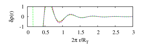
a)

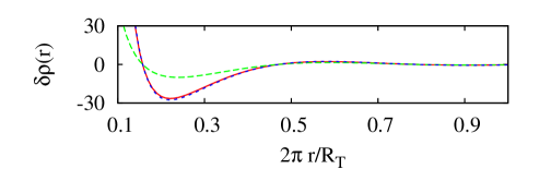
b)

Figure 2: (Color online) Variation of electronic density computed at finite temperature using the exact expression Eq. (72) [red solid line], the long distance coherent approximation Eq. (70) [blue doted line] which is appropriate for $R_{K}<r<R_{T}$, and the very long distance regime $r>R_{T}$ approximated by Eq. (73) [green dashed line]. a) Overview along few Friedel oscillations, b) Focus at relatively short distance. Here, we chose $R_{T}=50R_{K}$ and $\pi R_{F}=5R_{K}$.

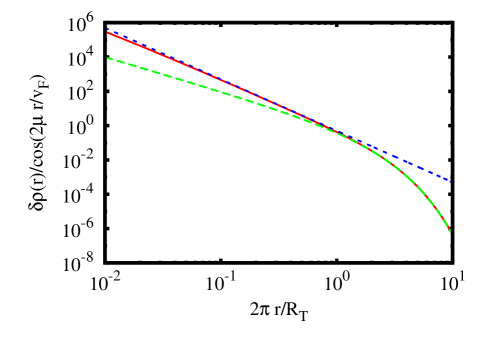
Figure 3: (Color online) Plot of the envelope of Friedel oscillations, $\delta\rho({\bf r})/\cos(2\mu r/v_{F})$, computed at finite temperature using the exact expression Eq. (72) [red solid line], the long distance coherent approximation Eq. (70) [blue dotted line] which is appropriate for $R_{K}<r<R_{T}$, and the very long distance regime $r>R_{T}$ approximated by Eq. (73) [green dashed line]. Here, we chose $R_{T}=50R_{K}$ and $\pi R_{F}=5R_{K}$.

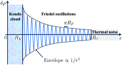
Figure 4: Schematic description of the Friedel oscillations that can be observed in the density variations around the impurity when $T<T_{K}$. For the rotationally invariant case $\lambda=0$ the envelope decays like $1/r^{3}$. For the warping term $\lambda\neq 0$ the decay is slower (like $1/r^{2}$) in some directions.

We see from the previous analysis that there are three relevant lengthscales as depicted schematically by figure 4. The first one, $R_{F}=v_{F}/\mu$, is proportional to the Fermi wavelength. For lengthscales much larger than $R_{F}$, the simplification (67) is justified, and $R_{F}$ then simply gives the pseudo-period of the Friedel oscillations. The second lengthscale is the Kondo screening length $R_{K}$, which is the size of the Kondo cloud; due to the temperature dependence of the Kondo resonance width, $\Gamma(T)$, we have $R_{K}(T\gtrsim T_{K})=\infty$ and $R_{K}(T\ll T_{K})\propto v_{F}/T_{K}$. Above that lengthscale, which requires at least $T<T_{K}$, the Friedel oscillations become identical to those of a resonant non-magnetic impurity. The third important lengthscale is the thermal length $R_{T}$. Beyond that length, the Friedel oscillations decay exponentially, while below $R_{T}$ they are unchanged from the zero temperature case. In order to observe the Friedel oscillations characteristic of the Kondo screening cloud, we must have $T\ll T_{K}$ so that the Kondo screening length is much shorter than the thermal length. In a renormalization group picture, the temperature is the natural infrared cutoff for the renormalization group flow, and the constraint $T\ll T_{K}$ is simply a requirement that the strong coupling scale is reached before the thermal cutoff.

III.3 Friedel oscillations with warping

We now turn to the electronic local density $\rho(\mathbf{r})$ in the presence of warping. For $\lambda\neq 0$ we don’t have anymore an expression in closed form of the Green’s function. Instead, we use the approximation (105) derived in App.B :

$$G_{0}(\mathbf{r},i\nu_{n})=G_{0}(r,\theta,i\nu_{n}) = \frac{i\nu_{n}+\mu}{2\pi v_{F}^{2}}\left[K_{0}(\zeta_{n})+\mathrm{sign}(\nu_{n})\mathbf{\hat{z}}\cdot(\boldsymbol{\sigma}\times\mathbf{\hat{r}})K_{1}(\zeta_{n})\right.$$ (75)

$$\left.+\lambda\sigma^{z}\cos(3\theta)(i\nu_{n}+\mu)^{2}\mathrm{sign}(\nu_{n})K_{3}(\zeta_{n})/v_{F}^{3}\right]+O(\lambda^{2})~{},$$

with

$$\zeta_{n} \equiv \frac{|\nu_{n}|-i\mu~{}\mathrm{sign}(\nu_{n})}{v_{F}}r~{}.$$ (76)

We obtain:

$$\mathrm{Tr}\left[G(r,\theta,i\nu_{n})G(r,\theta+\pi,i\nu_{n})\right]=\frac{(i\nu_{n}+\mu)^{2}}{2\pi^{2}v_{F}^{4}}\left[K_{0}\left(\frac{|\nu_{n}|-i\mu~{}\mathrm{sign}(\nu_{n})}{v_{F}}r\right)^{2}-K_{1}\left(\frac{|\nu_{n}|-i\mu~{}\mathrm{sign}(\nu_{n})}{v_{F}}r\right)^{2}\right.$$

$$-\left.\left(\frac{\lambda}{v_{F}}\cos 3\theta\right)^{2}\left(\frac{i\nu_{n}+\mu}{v_{F}}\right)^{4}K_{3}\left(\frac{|\nu_{n}|-i\mu~{}\mathrm{sign}(\nu_{n})}{v_{F}}r\right)^{2}\right]~{}.$$ (77)

Since this expression is only approximate, we cannot use contour integration techniques to obtain the sum (53). Indeed, attempting to use contour integration for $T>0$ yields a divergent integral. Nevertheless, for zero temperature, we can still change the sum (53) into an integral as the exponential decay of the modified Bessel function ensures the convergence of the sums. This leads to the zero temperature result valid for $r\gg R_{K}=v_{F}/\Gamma$ :

$$\delta\rho(\mathbf{r}) = \delta\rho(\mathbf{r})|_{\lambda=0}-\lambda^{2}\frac{\mu^{4}\cos^{2}(3\theta)}{4\pi^{2}v_{F}^{6}r^{2}}\cos\left(2\frac{\mu r}{v_{F}}\right)~{}.$$ (78)

For positive temperature, we have to compute the sum (53) numerically. This will be done in the next section using realistic values for the model parameters. Here we rather discuss general new features that emerge from this warping term. First, we expect finite temperature corrections to be relevant only in the crossover temperature regime around $T_{K}$. Indeed, similarly to what we found without warping, the thermal length $R_{T}=v_{F}/T$ provides a cut-off below which Friedel oscillations are identical to the ones predicted for $T=0$, and above which they are muffled by thermal fluctuations.

Furthermore, one important feature here in this expression is the $1/r^{2}$ decay of the envelope: this decay is identical to the one of a two-dimensional normal metal, and it dominates the $1/r^{3}$ contribution from the non-warping. Because of the $\cos^{2}3\theta$ factor, the Friedel oscillations in the directions $\theta=\frac{\pi}{6}(2n+1)$ have the contribution from warping switched off and contain only the $1/r^{3}$ contribution, whilst in other directions the warping contribution is observable and dominates on the longer lengthscales due to its slower $1/r^{2}$ decay.

Also, $R_{K}=v_{F}/\Gamma$ characterizing the size of the Kondo screening cloud, we expect the Friedel oscillations to be observable only at distance larger than this Kondo length. Within a renormalization group picture, the density oscillations are thus supposed to be measured at a sufficiently large distance from the Kondo impurity such that the system is correctly described by its strong coupling fixed point, i.e., the Kondo spin is totally screened. Nevertheless, comparing Eq. (70) and Eq. (78) we find that the warping correction becomes relevant only for distances larger than a new characteristic length, $R_{W}=\frac{v_{F}^{7}}{\lambda^{2}\mu^{5}}$. Introducing the density of surface states $n_{S}$ and invoking the density of states $\rho_{0}(E)=|E|/(2\pi v_{F}^{2})$ in the vicinity of the Dirac point, we have $n_{S}=\mu^{2}/(4\pi v_{F}^{2})=1/(4\pi R_{F}^{2})$, so that $R_{W}=(v_{F}/\lambda)^{2}(4\pi n_{S})^{-5/2}$. A crossover density emerges, $n_{S}^{\star}\equiv\frac{1}{4\pi}\left(\frac{v_{F}^{2}}{\lambda^{2}R_{K}}\right)^{2/5}$, that distinguishes two different cases: for $n_{S}>n_{S}^{\star}$, we find $R_{W}<R_{K}$ and the Friedel oscillations which are observed for $R_{K}<r<R_{T}$ are characterized by the warping term with switch on and off directions and an $1/r^{3}$ envelope. But, closer to the Dirac point, i.e., for density $n_{S}<n_{S}^{\star}$, Friedel oscillations are characterized by two regimes: at shortest distances $R_{K}<r<R_{W}$ the isotropic term with $1/r^{2}$ envelope dominates, whilst the warping correction dominates at larger distances $R_{W}<r<R_{T}$. Also, a new temperature scale emerges in the lowest density case $n_{S}<n_{S}^{\star}$: the warping temperature $T_{W}\equiv v_{F}/R_{W}<T_{K}$ indicating the crossover temperature below which warping effects appear.

IV Discussion

IV.1 Experimental observability of the density oscillations

Here we analyze the experimental observability of the density oscillation effects, with or without warping effects, that were discussed on general grounds in the previous section. The idea is to compute the density variation $\delta\rho({\bf r)}$ around a Kondo impurity using realistic values of parameters that correspond to topologically insulating compounds for which surface states have been observed or predicted. We consider more specifically two compounds: $\mathrm{Bi_{2}Se_{3}}$ for which Ref. kuroda2010, gives $v_{F}=3.55$ eVÅ and $\lambda=128$ eVų, and $\mathrm{Bi_{2}Te_{3}}$ with values $v_{F}=2.55$ eVÅ and $\lambda=250$ eVų given by Refs. chen2009, and an2012, . We are still left with two tunable parameters: the Kondo temperature $T_{K}=v_{F}/R_{K}$, and the density of surface states $n_{S}=\mu^{2}/(4\pi v_{F}^{2})=1/(4\pi R_{F}^{2})$. First, we remark that the Kondo temperature depends on various microscopic parameters including the chemistry of the magnetic impurity and the density $n_{S}$. Furthermore the well know exponential $J_{K}-$dependence of $T_{K}$ (see section III.1.2) makes this temperature scale very sensitive to variations of these microscopic parameters. Therefore, refereeing from the orders of magnitude that are usually measured in Kondo compounds we consider here three different characteristic values: $T_{K}=1000$ K (big), $T_{K}=100$ K (medium), and $T_{K}=10$ K (relatively small). For the density of surface states $n_{S}$, we consider three values for each compound: the crossover density $n_{S}^{\star}=\frac{1}{4\pi}\left(\frac{v_{F}^{2}}{\lambda^{2}R_{K}}\right)^{2/5}$, a smaller density $n_{S}=n_{S}^{\star}/10$, and a larger density $n_{S}=10n_{S}^{\star}$. The sets of relevant parameters that we consider are summarized in table 1 for $\mathrm{Bi_{2}Se_{3}}$, and in table 2 for $\mathrm{Bi_{2}Te_{3}}$.

	$T_{K}=10$ K	$T_{K}=100$ K	$T_{K}=1000$ K
	$R_{K}=410$ nm	$R_{K}=41$ nm	$R_{K}=4,1$ nm
$n_{S}\approx n_{S}^{\star}/10$	$n_{S}=1,6.10^{3}$ $\mu$m-2	$n_{S}=4.10^{3}$ $\mu$m-2	$n_{S}=10^{4}$ $\mu$m-2
	$\mu=50$ meV	$\mu=80$ meV	$\mu=130$ meV
	$R_{F}=7,0$ nm	$R_{F}=4,4$ nm	$R_{F}=2,8$ nm
	$R_{W}=130$ $\mu$m	$R_{W}=13$ $\mu$m	$R_{W}=1,3$ $\mu$m
	$T_{W}=3.10^{-5}$ K	$T_{W}=3.10^{-4}$ K	$T_{W}=3.10^{-3}$ K
$n_{S}\approx n_{S}^{\star}$	$n_{S}=1,6.10^{4}$ $\mu$m-2	$n_{S}=4.10^{4}$ $\mu$m-2	$n_{S}=10^{5}$ $\mu$m-2
	$\mu=160$ meV	$\mu=250$ meV	$\mu=400$ meV
	$R_{F}=2,2$ nm	$R_{F}=1,4$ nm	$R_{F}=8,8$ Å
	$R_{W}=410$ nm	$R_{W}=41$ nm	$R_{W}=4,1$ nm
$n_{S}\approx 10n_{S}^{\star}$	$n_{S}=1,6.10^{5}$ $\mu$m-2	$n_{S}=4.10^{5}$ $\mu$m-2	$n_{S}=10^{6}$ $\mu$m-2
	$\mu=500$ meV	$\mu=800$ meV	$\mu=1,3$eV
	$R_{F}=7,0$ Å	$R_{F}=4,4$ Å	$R_{F}=2,8$ Å
	$R_{W}=1,3$ nm	$R_{W}=1,3$ Å	$R_{W}=0,13$ Å

Table 1: Model parameters for $\mathrm{Bi_{2}Se_{3}}$, with $v_{F}=3.55$ eVÅ and $\lambda=128$ eVų.

	$T_{K}=10$ K	$T_{K}=100$ K	$T_{K}=1000$ K
	$R_{K}=300$ nm	$R_{K}=30$ nm	$R_{K}=3$ nm
$n_{S}\approx n_{S}^{\star}/10$	$n_{S}=8,3.10^{2}$ $\mu$m-2	$n_{S}=2,1.10^{3}$ $\mu$m-2	$n_{S}=5,2.10^{3}$ $\mu$m-2
	$\mu=26$ meV	$\mu=41$ meV	$\mu=65$ meV
	$R_{F}=9,8$ nm	$R_{F}=6,2$ nm	$R_{F}=3,9$ nm
	$R_{W}=94$ $\mu$m	$R_{W}=9,4$ $\mu$m	$R_{W}=940$ nm
	$T_{W}=3.10^{-5}$ K	$T_{W}=3.10^{-4}$ K	$T_{W}=3.10^{-3}$ K
$n_{S}\approx n_{S}^{\star}$	$n_{S}=8,3.10^{3}$ $\mu$m-2	$n_{S}=2,1.10^{4}$ $\mu$m-2	$n_{S}=5,2.10^{4}$ $\mu$m-2
	$\mu=82$ meV	$\mu=130$ meV	$\mu=210$ meV
	$R_{F}=3,1$ nm	$R_{F}=2,0$ nm	$R_{F}=1,2$ nm
	$R_{W}=300$ nm	$R_{W}=30$ nm	$R_{W}=3$ nm
$n_{S}\approx 10n_{S}^{\star}$	$n_{S}=8,3.10^{4}$ $\mu$m-2	$n_{S}=2,1.10^{5}$ $\mu$m-2	$n_{S}=5,2.10^{5}$ $\mu$m-2
	$\mu=260$ meV	$\mu=410$ meV	$\mu=650$ meV
	$R_{F}=9,8$ Å	$R_{F}=6,2$ Å	$R_{F}=3,9$ Å
	$R_{W}=9,3$ Å	$R_{W}=0,93$ Å	$R_{W}=0,093$ Å

Table 2: Model parameters for $\mathrm{Bi_{2}Te_{3}}$, with $v_{F}=2.55$ eVŠand $\lambda=250$ eVų.

The results are represented on Figs. 5 and 6 for $\mathrm{Bi_{2}Se_{3}}$ and $\mathrm{Bi_{2}Te_{3}}$ respectively. For these plots, we fixed arbitrarily $T_{K}=100$ K and we chose realistic relevant values of chemical potential $\mu$, that can be controlled experimentally by doping with Snchen2009 or Mgkuroda2010 . In $\mathrm{Bi_{2}Se_{3}}$ compounds, experimental values of $\mu$ indicated in Ref. kuroda2010, are tuned from $350$ meV down to $0$ eV. Therefore, the four values that we considered for the plots of Fig. 5 were chosen invoking table 1 in order to illustrate the observability of the various cases: with dominant warping term ($\mu=350$ meV$>\mu^{\star}$), with similar warping and isotropic terms ($\mu=\mu^{\star}=250$ meV), and with negligible warping term ($\mu=130$ meV, and $50$ meV). Figure 5 clearly shows the Friedel oscillations with six-fold rotation symmetry when $\mu>\mu^{\star}$, or with full rotation symmetry when $\mu<\mu^{\star}$. The choice of $T_{K}=100$ K for this plot is arbitrary and experimental values of the Kondo temperature can be significantly different. Furthermore, we are aware that doping, i.e., varying $\mu$, strongly affects the value of $T_{K}$ which may continuously vanish at the Dirac point as we discussed in section III.1.2. Nevertheless, we expect that the Friedel oscillations will qualitatively not really depend on $T_{K}$. This is a consequence of the universality of the strong Kondo coupling effective regime that is realized below $T_{K}$ within the renormalization group picture: since Friedel oscillations appear above the Kondo screening size $R_{K}$ their shape is qualitatively universal (but still depends on the warping length $R_{W}$ and Fermi pseudo period $\pi R_{F}$). Also, according to the values given in table 1, the crossover value for the chemical potential varies very smoothly from $\mu^{\star}=160$ meV to $\mu^{\star}=400$ meV when $T_{K}$ changes from $10$ K to $1000$ K. This suggests that the results which are illustrated by figure 5 for $T_{K}=100$ K can be extended to any other values of $T_{K}$. Of course, the characteristic unit length which is used for the plots, $R_{K}$, would have to be rescaled accordingly. Experimentally, one of the main difficulties for observing Friedel oscillations with or without six-fold symmetry is the requirement of cooling the temperature sufficiently lower than $T_{K}$, but the orders of magnitudes that are considered here correspond to values that are realistic both physically ($T_{K}$ is imposed by the chemistry) and technologically ($T$ is limited by cryogenic technics).

We made a similar analysis for $\mathrm{Bi_{2}Te_{3}}$ compounds. In this case, Ref. chen2009, indicates experimental values of $\mu$ between $350$ meV and $120$ meV. We thus plotted these two extreme cases, together with the intermediate value $\mu=250$ meV. Here, we chose a Kondo temperature $T_{K}=100$ K, which corresponds to a crossover value $\mu^{\star}=130$ meV as indicated in table 2. In this case, the six-fold symmetry resulting from the warping is thus observable for $\mu=350$ meV and $250$ meV, and the full rotation symmetry is recovered for $\mu=120$ meV. The six-fold symmetry may remain for that value of chemical potential if the Kondo temperature is lowered. Indeed, table 2 indicates $\mu^{\star}=82$ meV for $\mathrm{Bi_{2}Te_{3}}$ compounds with $T_{K}=10$ K.

Here, we have restricted our analysis to the observation of Friedel oscillations within the fluctuation of the local density of states, $\delta\rho({\bf r})$. This physical quantity can be measured experimentally using Scanning Tunneling Microscopy (STM). Local Density of Statesmitchell2012 (LDOS) measurements have already been performed by STM on Kondo impurities at the surface of metals.madhavan1998 ; madhavan2001 ; knorr2002 ; wahl2005 ; ysfu2007 The measurement of the Friedel oscillations would require the integration of the measured local density of states over a range of energyaffleck2008 . Beside the issue of cooling the temperature sufficiently lower than $T_{K}$, other technical limitations have to be considered in order to observe the predicted Friedel oscillations using STM:
First, a voltage bias is applied locally between the tip of the STM and the surface of the sample. The resulting STM current which is measured may invoke out of equilibrium effects that have not been analyzed here. We expect our predictions to be valid for STM experiments with bias voltages invoking energies that are lower to both $T_{K}$ and $\mu$. Higher values of bias voltage may have non universal effects on the Kondo screening leading to a distortion of the Friedel oscillations.
A second limitation is the STM resolution in both lateral and depth directions. More precisely, we may expect an experimental STM measurement of the Friedel oscillations to be realized by moving the STM tip at the surface of the system along two orthogonal directions. The most natural resulting STM signal will thus be discretized on a grid having a square lattice symmetry and an elementary step of length $R_{STM}\simeq 0.2$nm. Since the period of the Friedel oscillations is $\pi R_{F}$, the measured STM signal may exhibit a Moiré patternkuwabara1990 resulting from the interference between the two periods, $R_{STM}$ and $\pi R_{F}$. Considering the values of $R_{F}$ which are given in tables 1 and 2, and assuming $R_{STM}$ is of the order of one or few Å, Moiré patterns might occur for values of chemical potential relatively higher than $\mu^{\star}$. In such cases, the measured STM images would only have the two-fold symmetry common to both the square and the hexagonal symmetry groups.

Comparing qualitatively the plots of figures 5 and 6, we find that warping effects and their related six-fold symmetry are more observable at the surface of Bi₂Te₃ rather than Bi₂Se₃. This is due of course to a larger value of the warping constant $\lambda$, but this also results from a smaller value of the Fermi velocity $v_{F}$, which gives a smaller value of crossover potential $\mu^{\star}$.

Figure 5: Intensity plot of the Friedel oscillations around a screened magnetic impurity at the edge of $\mathrm{Bi_{2}Se_{3}}$. Model parameters $v_{F}=3.55$ eVÅ and $\lambda=128$ eVų. We chose $T_{K}=100K$ and $T=10K$. From top left to bottom right, $\mu=350$ meV, $250$ meV, $130$ meV, $50$ meV. Unit length: $R_{K}$. Short distances, $r<0.2R_{K}$, are not represented. Intensity in arbitrary units is represented by the darkness of the plots.

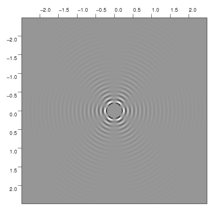
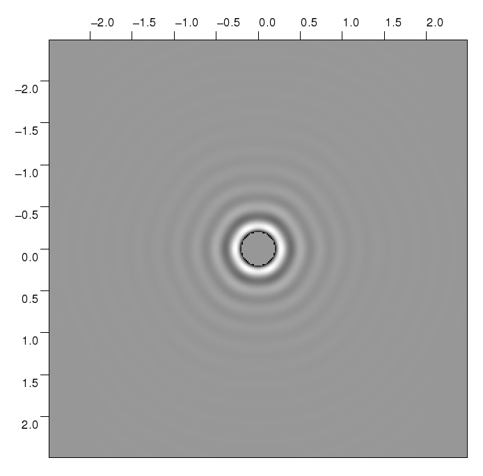
Figure 6: Intensity plot of the Friedel oscillations around a screened magnetic impurity at the edge of $\mathrm{Bi_{2}Te_{3}}$. Model parameters $v_{F}=2.55$ eVÅ and $\lambda=250$ eVų. We chose $T_{K}=100K$ and $T=10K$. From left to right, $\mu=340$ meV, $250$ meV, $120$ meV. Unit length: $R_{K}$. Short distances, $r<0.2R_{K}$, are not represented. Intensity in arbitrary units is represented by the darkness of the plots.

IV.2 Conclusion

We have shown that a magnetic impurity on the surface of a strong topological insulator will be fully screened by the surface modes unless the Fermi energy is exactly at the Dirac point. The result depends only on the time reversal invariance of the effective Hamiltonian of the surface modes and is valid in particular in the presence of warping of the Fermi surface. We have shown that Friedel oscillations are formed around the impurity and we have calculated the shape of these oscillations both without warping and with a weak warping that can be treated perturbatively. With warping, the symmetry of the Friedel oscillation pattern is broken from full rotational symmetry to a six-fold symmetry. In both cases, the pseudo period of the oscillations, $\pi R_{F}=\pi v_{F}/\mu$, is half the Fermi wave length of the surface modes, the short distance cut-off $R_{K}\propto v_{F}/T_{K}$ is determined by the Kondo temperature $T_{K}$, and the long distance cut-off $R_{T}=v_{F}/T$ results from thermal fluctuations. With warping, the amplitude of the fully rotationally symmetric part decreases as $1/r^{3}$, whilst the 6-fold symmetry term has an envelope decreasing more slowly, a $1/r^{2}$. As a consequence, a new length scale $R_{W}$ emerges, above which Friedel oscillations with six-fold symmetry may be observed. The crossover condition $R_{K}\approx R_{W}$ defines a chemical potential $\mu^{\star}$ associated to a doping $n_{S}^{\star}$ above which the Friedel oscillations are characterized by the six-fold symmetry even at shortest distances. Considering realistic values for the model parameters, we analyzed the observability and the symmetry of Friedel oscillations in the vicinity of magnetic impurities deposited at the surface of two compounds, $\mathrm{Bi_{2}Se_{3}}$ and $\mathrm{Bi_{2}Te_{3}}$. We identified large range of parameters where the crossover between the 6-fold and the fully rotational symmetries may be observed. We propose to use STM as an experimental probe for the variation of the local density of states.

Various questions remain to be addressed. First, it would be interesting to investigate the unstable fixed point that separates the regime with Kondo screening from the regime of decoupled impurities in the case of a system at half-filling. Second, an exact calculation of the Friedel oscillations could be performed using form factor expansion methodsmussardo_offcritical_review ; saleur_cambridge at zero temperature.

The single impurity model that we considered here could also be generalized to two or several impurities. In this case, the local Kondo screening will compete with the Ruderman-Kittel-Kasuya-Yosidaruderman1954 ; kasuya1956 ; yosida1957 (RKKY) inter-impurity screening as discussed by Doniachdoniach1977 in a general context. Here, we may expect the 6-fold symmetry of the Friedel oscillations to have signatures on the symmetry of the RKKY interaction.

Appendix A Details of the mean-field approximation

We start from the mean-field self-consistent relations (43):

$$|\Delta|^{2} = J_{K}\int_{-\infty}^{\infty}\frac{dE}{\pi}\frac{(E+\mu_{f})n_{F}(E)\Sigma^{\prime\prime}(E)}{[E+\mu_{f}-\Sigma^{\prime}(E)]^{2}+[\Sigma^{\prime\prime}(E)]^{2}}~{},$$ (79)

$$\frac{1}{2} = -\int_{-\infty}^{\infty}\frac{dE}{\pi}\frac{n_{F}(E)\Sigma^{\prime\prime}(E)}{[E+\mu_{f}-\Sigma^{\prime}(E)]^{2}+[\Sigma^{\prime\prime}(E)]^{2}}~{},$$ (80)

with the expression (42) of the imaginary part of the self energy:

$$\Sigma^{\prime\prime}(E) = -\pi|\Delta|^{2}\rho_{0}(\mu+E)~{}.$$ (81)

Introducing the Hilbert transform of the density of states:

$$\Phi(E)\equiv\int_{-\infty}^{\infty}d\epsilon\rho_{0}(\epsilon)\mathrm{P.V.}\left(\frac{1}{E-\epsilon}\right)~{},$$ (82)

the expression (41) of the real part of the self-energy can be written as:

$$\Sigma^{\prime}(E) = \pi|\Delta|^{2}\Phi(\mu+E)~{}.$$ (83)

A.1 Derivation of the Kondo temperature

When the temperature $T$ goes to $T_{K}$, the hybridization parameter $\Delta$ vanishes. In such limit, the Eq. (80) reduces to $n_{F}(-\mu_{F})=1/2$, yielding $\mu_{f}(T_{K})=0$. The Eq. (79) can then be cast into the Nagaoka-Suhl formnagaoka_resonance ; suhl_resonance :

$$-\frac{1}{J_{K}}=\mathrm{P.V.}\int_{-\infty}^{+\infty}\frac{dE}{E}n_{F}(E)\rho_{0}(\mu+E)$$ (84)

In the general $\mu>0$ case, we can rewrite Eq. (84):

$$-\frac{1}{J_{K}} = -\rho_{0}(\mu)\int_{0}^{D-\mu}\frac{dE}{2E}\tanh\left(\frac{E}{2T_{K}}\right)-\rho_{0}(\mu)\int_{D-\mu}^{D+\mu}\frac{dE}{E}n_{F}(-E)$$ (85)

$$+\int_{-D-\mu}^{D-\mu}\frac{dE}{E}[\rho_{0}(\mu+E)-\rho_{0}(\mu)]n_{F}(E)~{},$$

where $D$ is a bandwidth cutoff such that $\rho(E)=0$ when $|E|>D$. taking the limit of low Kondo temperature $T_{K}\ll D,\mu$, we obtain the following approximate equation:

$$\frac{1}{J_{K}}=\rho_{0}(\mu)\ln\left(\frac{2e^{\gamma_{E}}(D+\mu)}{\pi T}\right)-\int_{-D-\mu}^{0}\frac{dE}{E}[\rho_{0}(\mu+E)-\rho_{0}(\mu)]~{},$$ (86)

improving the prefactor in the expression of the Kondo temperature by taking into account the variation of the density of states with the energy.

A.2 Derivation of the resonance width

We have seen that both $\Gamma$ and $\mu_{f}$ vanish at and above the Kondo temperature. Hereafter, we will consider the limit of small Kondo coupling, and we will thus assume that $\Gamma$ and $\mu_{f}$ remain small compared to the non-interacting electron characteristic energy scales, even below the Kondo temperature where these quantities are not vanishing any more. If we take first the equation (80), and make the approximations $\Sigma^{\prime}(E)=0$, $\Sigma"(E)=\Sigma"(0)=-\Gamma$, we obtain:

$$\frac{1}{2}=\int_{-\infty}^{\infty}\frac{dE}{\pi}\frac{\Gamma}{(E+\mu_{f})^{2}+\Gamma^{2}}n_{F}(E)\simeq n_{F}(-\mu_{f})~{},$$ (87)

so we have to take also $\mu_{f}=0$. Inserting our approximations in the denominator of (79), we obtain a second equation:

$$-\frac{1}{J_{K}}=\int_{-\infty}^{\infty}dE\frac{En_{F}(E)\rho_{0}(\mu+E)}{E^{2}+\Gamma^{2}}~{}.$$ (88)

We introduce the bandwidth cutoff $D$ such that $\rho_{0}(E)=0$ if $|E|>D$. We can then rewrite Eq. (88) in the form:

$$-\frac{1}{J_{K}}=\rho_{0}(\mu)\int_{-D-\mu}^{D-\mu}dE\frac{En_{F}(E)}{E^{2}+\Gamma^{2}}+\int_{-D-\mu}^{D-\mu}dE\frac{En_{F}(E)[\rho_{0}(\mu+E)-\rho_{0}(\mu)]}{E^{2}+\Gamma^{2}}~{}.$$ (89)

In the rightmost integral of the right hand side, $\rho(\mu+E)-\rho(\mu)$ vanishes for $E=0$, so we can neglect $\Gamma$ in the denominator. This gives the final equation:

$$-\frac{1}{J_{K}\rho_{0}(\mu)}=\int_{-D-\mu}^{D-\mu}\frac{En_{F}(E)}{E^{2}+\Gamma^{2}}dE+\int_{-D-\mu}^{D-\mu}\frac{\rho(E+\mu)-\rho(\mu)}{\rho_{0}(\mu)}n_{F}(E)\frac{dE}{E}~{}.$$ (90)

With that approximation, and taking the zero temperature limit, we obtain:

$$\Gamma(T=0)=(D+\mu)\exp\left[-\frac{1}{J_{K}\rho_{0}(\mu)}-\int_{-D-\mu}^{0}\frac{dE}{E}\frac{\rho_{0}(\mu+E)-\rho_{0}(\mu)}{\rho_{0}(\mu)}\right]~{}.$$ (91)

We note that $\Gamma(T=0)/T_{K}=2e^{\gamma_{E}}/\pi\simeq 2.26$ for such level of approximation. For finite temperature, we can replace $n_{F}(E)$ with $\theta(-E)$ in the integral over the density of states in the right-hand side of Eq. (90). Using that approximation, we can write:

$$\ln\left(\frac{\Gamma(T=0)}{\Gamma(T)}\right)=\int_{-\infty}^{\infty}\frac{du}{4\cosh^{2}u}\ln\left(1+\frac{4T^{2}u^{2}}{\Gamma^{2}}\right)~{}.$$ (92)

These equations imply that $\Gamma(T)=\Gamma(T=0)\varphi(\Gamma(T=0)/T)$, so given the relation between $\Gamma(T=0)$ and $T_{K}$, $\Gamma(T)=\Gamma(T=0)\bar{\varphi}(T_{K}/T)$.

Appendix B Asymptotic approximation for the Green’s function in the presence of warping

The exact Green’s function of the surface electrons is:

$$G_{0}(\mathbf{r},i\nu_{n})=\int\frac{d^{2}\mathbf{k}}{(2\pi)^{2}}\frac{i\nu_{n}+\mu+v_{F}\mathbf{\hat{z}}\cdot(\boldsymbol{\sigma}\times\mathbf{k})+\frac{\lambda}{2}(k_{+}^{3}+k_{-}^{2})\sigma^{z}}{(i\nu_{n}+\mu)^{2}-v_{F}^{2}k^{2}-\left[\frac{\lambda}{2}(k_{+}^{3}+k_{-}^{2})\right]^{2}}e^{i\mathbf{k}\cdot\mathbf{r}}~{}.$$ (93)

Using polar coordinates, we can express the Green’s function (93) as a series:

$$G_{0}(r,\theta,i\nu_{n}) = \int\frac{kdk}{(2\pi)^{2}}\int d\phi\frac{iz+iv_{F}k(\sigma^{+}e^{-i\phi}-\sigma_{-}e^{i\phi})+\lambda k^{3}\cos(3\phi)\sigma^{z}}{\sqrt{(z^{2}+v_{F}^{2}k^{2})(z^{2}+v_{F}^{2}k^{2}+\lambda^{2}k^{6})}}e^{ikr\cos(\phi-\theta)}\times$$ (94)

$$\sum_{m=-\infty}^{\infty}\left(\frac{\lambda^{2}k^{6}}{(\sqrt{(z^{2}+v_{F}^{2}k^{2})}+\sqrt{(z^{2}+v_{F}^{2}k^{2}+\lambda^{2}k^{6})})^{2}}\right)^{|m|}(-e^{i6\phi})^{m}~{},$$

where $z=\nu_{n}-i\mu$. To obtain an asymptotic expansion of $G(r,\theta,i\nu_{n})$ to lowest order in $\lambda$ it is enough to consider the term $m=0$. We then have to consider the integral:

$$G_{0}(r,\theta,i\nu_{n})=\int\frac{kdk}{(2\pi)^{2}}\int d\phi\frac{iz+iv_{F}k(\sigma^{+}e^{-i\phi}-\sigma_{-}e^{i\phi})+\lambda k^{3}\cos(3\phi)\sigma^{z}}{\sqrt{(z^{2}+v_{F}^{2}k^{2})(z^{2}+v_{F}^{2}k^{2}+\lambda^{2}k^{6})}}e^{ikr\cos(\phi-\theta)}+\cdots~{},$$ (95)

where $\cdots$ denotes corrections of higher order in $\lambda$. After integration with respect to $\phi$ this expression gives:

$$G_{0}(r,\theta,i\nu_{n}) = \int_{0}^{\infty}dk\frac{izkJ_{0}(kr)-v_{F}k^{2}(\sigma^{+}e^{-i\theta}-\sigma_{-}e^{i\theta})J_{1}(kr)-i\lambda k^{4}\cos(3\theta)\sigma^{z}J_{3}(kr)}{2\pi\sqrt{(z^{2}+v_{F}^{2}k^{2})(z^{2}+v_{F}^{2}k^{2}+\lambda^{2}k^{6})}}$$

$$\equiv \frac{iz}{2\pi}I-\frac{v_{F}}{2\pi}(\sigma^{+}e^{-i\theta}-\sigma_{-}e^{i\theta})I^{\prime}-\frac{i\lambda}{2\pi}\cos(3\theta)\sigma^{z}I^{\prime\prime}~{}.$$ (97)

In the limit $\lambda\to 0$, we have from Eq. (11.4.44) in Ref. abramowitz_math_functions, :

$$I \to \int_{0}^{\infty}dk\frac{kJ_{0}(kr)}{z^{2}+v_{F}^{2}k^{2}}=\frac{1}{v_{F}^{2}}K_{0}\left(\frac{|\nu_{n}|-i\mu~{}\mathrm{sign}(\nu_{n})}{v_{F}}r\right)~{},$$ (98)

$$I^{\prime} \to \int_{0}^{\infty}dk\frac{k^{2}J_{1}(kr)}{z^{2}+v_{F}^{2}k^{2}}=\frac{|\nu_{n}|-i\mu~{}\mathrm{sign}(\nu_{n})}{v_{F}^{3}}K_{1}\left(\frac{|\nu_{n}|-i\mu~{}\mathrm{sign}(\nu_{n})}{v_{F}}r\right)~{},$$ (99)

with corrections of order $\lambda^{2}$. We are thus left with the evaluation of the integral:

$$I^{\prime\prime}=\int_{0}^{+\infty}\frac{k^{4}J_{3}(kr)dk}{\sqrt{(z^{2}+(v_{F}k)^{2})(z^{2}+(v_{F}k)^{2}+\lambda^{2}k^{6})}}~{}.$$ (100)

In the expression (100) we cannot take the limit $\lambda\to 0$ directly before integrating as we would obtain a divergent integral. Instead, we will first make integrations by parts using Eq. (9.1.30) in Ref. abramowitz_math_functions, to obtain an asymptotic expansion. The first integration by parts gives:

$$I^{\prime\prime} = \frac{1}{r}\int_{0}^{+\infty}dkk^{4}J_{4}(kr)\left[\frac{v_{F}^{2}k}{(z^{2}+v_{F}^{2}k^{2})^{3/2}(z^{2}+v_{F}^{2}k^{2}+\lambda^{2}k^{6})^{1/2}}+\frac{v_{F}^{2}k+3\lambda^{2}k^{5}}{(z^{2}+v_{F}^{2}k^{2})^{1/2}(z^{2}+v_{F}^{2}k^{2}+\lambda^{2}k^{6})^{3/2}}\right]~{}.$$

$$= \frac{v_{F}^{2}}{r}\int_{0}^{+\infty}dkk^{5}J_{4}(kr)\left[\frac{1}{(z^{2}+v_{F}^{2}k^{2})^{3/2}(z^{2}+v_{F}^{2}k^{2}+\lambda^{2}k^{6})^{1/2}}+\frac{1}{(z^{2}+v_{F}^{2}k^{2})^{1/2}(z^{2}+v_{F}^{2}k^{2}+\lambda^{2}k^{6})^{3/2}}\right]+\cdots~{},$$

where $\cdots$ denotes the third term in (LABEL:eq:annexe-Iseconde), which will be shown to be negligible in the limit $\lambda\to 0$ in App. C. Using another integration by parts, we thus have:

$$I^{\prime\prime} \simeq \frac{v_{F}^{2}}{r^{2}}\int_{0}^{+\infty}k^{5}J_{5}(kr)\left[\frac{3v_{F}^{2}k}{(z^{2}+v_{F}^{2}k^{2})^{5/2}(z^{2}+v_{F}^{2}k^{2}+\lambda^{2}k^{6})^{1/2}}+\frac{v_{F}^{2}k+3\lambda^{2}k^{5}}{(z^{2}+v_{F}^{2}k^{2})^{3/2}(z^{2}+v_{F}^{2}k^{2}+\lambda^{2}k^{6})^{3/2}}\right]$$ (103)

$$+\frac{v_{F}^{2}}{r^{2}}\int_{0}^{+\infty}k^{5}J_{5}(kr)\left[\frac{v_{F}^{2}k}{(z^{2}+v_{F}^{2}k^{2})^{3/2}(z^{2}+v_{F}^{2}k^{2}+\lambda^{2}k^{6})^{3/2}}+\frac{3(v_{F}^{2}k+3\lambda^{2}k^{5})}{(z^{2}+v_{F}^{2}k^{2})^{1/2}(z^{2}+v_{F}^{2}k^{2}+\lambda^{2}k^{6})^{5/2}}\right]$$

If we take the limit $\lambda\to 0$ (justification for this can be found in App. C) in the above expression, we obtain a convergent integral:

$$I^{\prime\prime}\to\frac{8v_{F}^{4}}{r^{2}}\int_{0}^{+\infty}\frac{k^{6}J_{5}(kr)}{(z^{2}+v_{F}^{2}k^{2})^{3}}=\frac{(|\nu_{n}|-i\mu~{}\mathrm{sign}(\nu_{n}))^{3}}{v_{F}^{5}}K_{3}\left(\frac{|\nu_{n}|-i\mu~{}\mathrm{sign}(\nu_{n})}{v_{F}}r\right)~{}.$$ (104)

We can check that the terms proportional to $\lambda^{2}$ give contributions that are vanishing in the limit $\lambda\to 0$.

Invoking the asymptotic expressions (98), (99), and (104) together in Eq. (97), we obtain the following approximation for the Green’s function in the limit of small warping:

$$G(r,\theta,i\nu_{n}) \simeq \frac{i\nu_{n}+\mu}{2\pi v_{F}^{2}}\left[K_{0}\left(\frac{|\nu_{n}|-i\mu~{}\mathrm{sign}(\nu_{n})}{v_{F}}r\right)+i(\sigma^{+}e^{-i\theta}-\sigma^{-}e^{i\theta})K_{1}\left(\frac{|\nu_{n}|-i\mu~{}\mathrm{sign}(\nu_{n})}{v_{F}}r\right)\mathrm{sign}(\nu_{n})\right.$$ (105)

$$+\left.\frac{\lambda}{v_{F}}\sigma^{z}\left(\frac{i\nu_{n}+\mu}{v_{F}}\right)^{2}K_{3}\left(\frac{|\nu_{n}|-i\mu~{}\mathrm{sign}(\nu_{n})}{v_{F}}r\right)\mathrm{sign}(\nu_{n})\cos 3\theta\right]~{}.$$

Appendix C Evaluation of the remainders

We consider the integral giving the remainder in Eq.(LABEL:eq:annexe-Iseconde):

$$I_{3}=\frac{3\lambda^{2}}{r}\int_{0}^{+\infty}dk\frac{k^{9}J_{4}(kr)}{(z^{2}+(vk)^{2})^{1/2}(z^{2}+(vk)^{2}+\lambda^{2}k^{6})^{3/2}}.$$ (106)

With the change of variables $k=\sqrt{v_{F}/\lambda}u$, the integral $I_{3}$ is rewritten:

$$I_{3}=\frac{3}{\lambda v_{F}r}\int_{0}^{+\infty}du\frac{u^{9}J_{4}(au)}{(b^{2}+u^{2})^{1/2}(b^{2}+u^{2}+u^{6})^{3/2}},$$ (107)

with $a=r(v_{F}/\lambda)^{1/2}$ and $b^{2}=\lambda z^{2}/v_{F}^{3}$. To obtain an upper bound for the integral, we use 3 successive integration by parts to rewrite:

$$I_{3}=\frac{3}{a^{3}\lambda v_{F}r}\int_{0}^{+\infty}du\frac{u^{7}J_{7}(ua)P(u)}{(b^{2}+u^{2})^{7/2}(b^{2}+u^{2}+u^{6})^{9/2}},$$ (108)

where the polynomial $P(u)$ has the expression:

$$P(u) = 480\,u^{22}+1200\,b^{2}\,u^{20}+1050\,b^{4}\,u^{18}-360\,u^{18}+315\,b^{6}\,u^{16}-3276\,b^{2}\,u^{16}-7200\,b^{4}\,u^{14}-6084\,b^{6}\,u^{12}-432\,b^{2}\,u^{12}$$ (109)

$$-1800\,b^{8}\,u^{10}-432\,b^{4}\,u^{10}+1152\,b^{6}\,u^{8}-96\,b^{2}\,u^{8}+1872\,b^{8}\,u^{6}-192\,b^{4}\,u^{6}+720\,b^{10}\,u^{4}+192\,b^{8}\,u^{2}+96\,b^{10}~{}.$$

The numerator in Eq. (108) is $O(u^{57/2})$ while the denominator is $O(u^{34})$ for $u\to\infty$ making the integral in (108) convergent. Moreover, an upper bound for the integral is given by:

$$\int_{0}^{+\infty}du\frac{|P(u)|}{\sqrt{2}(b^{2}+u^{2}+u^{6})^{9/2}}~{},$$ (110)

where we have used the inequalitiesabramowitz_math_functions $|J_{7}(u)|<1/\sqrt{2}$ and $(b^{2}+u^{2})^{-7/2}<u^{-7}$.We can them majorize the polynomial $P(u)$ by the sum of the absolute value of its monomials. For monomials of degree $n\geq 9$, we can also use the inequality $(b^{2}+u^{2}+u^{6})^{9/2}>u^{9}(1+u^{4})$ to obtain an upper bound larger than $b$. For the monomials of degree $n<8$, we obtain an upper bound of the form:

$$b^{m}\int_{0}^{+\infty}\frac{u^{n}du}{(b^{2}+u^{2}+u^{6})^{9/2}}<b^{m}\int_{0}^{+\infty}\frac{u^{n}du}{(b^{2}+u^{2})^{9/2}}=b^{n+m-8}\int_{0}^{+\infty}\frac{u^{n}du}{(1+u^{2})^{9/2}}~{}.$$ (111)

From the expression (109) of $P(u)$, we see that these terms contribute expressions $O(b^{2})$. In the case of $n=8$, we have to consider:

$$\int_{0}^{+\infty}\frac{u^{n}du}{(b^{2}+u^{2}+u^{6})^{9/2}}\leq\int_{0}^{1/b}du\frac{u^{8}}{(1+u^{2})^{9/2}}+\int_{1}^{+\infty}\frac{du}{u(1+u^{4})^{9/2}}~{}.$$ (112)

Inspecting the polynomial $P(u)$, we see that the contribution of the $u^{8}$ terms will be $O(b^{2}|\ln b|)$. Putting all contributions together, we see that:

$$I_{3} \leq \frac{3}{a^{3}\lambda v_{F}r}(C+O(b^{2}|lnb|))$$ (113)

$$\leq \frac{3}{v_{F}^{2}r^{3}}\sqrt{\frac{\lambda}{v_{F}}}(C+O(\lambda|\ln\lambda|)~{},$$ (114)

So $I_{3}=O(\lambda^{1/2})$ for $\lambda\to 0$. This establishes that this term gives a subdominant contribution to the Matsubara Green’s function.

We can apply the same method to the remainder integrals appearing in Eq. (103).

If we consider the integral:

$$I_{4}=\int_{0}^{\infty}\frac{\lambda^{2}k^{10}J_{5}(kr)}{(z^{2}+v_{F}^{2}k^{2})^{3/2}(z^{2}+v_{F}^{2}k^{2}+\lambda^{2}k^{6})^{3/2}}~{},$$ (115)

by the same change of variables $k=(v/\lambda)^{1/2}u$, we can transform it into:

$$I_{4}=\frac{1}{v_{F}^{7/2}\lambda^{1/2}}\int_{0}^{+\infty}\frac{u^{10}J_{5}(ua)}{(b^{2}+u^{2})^{3/2}(b^{2}+u^{2}+u^{6})^{3/2}}~{}.$$ (116)

Integrating by parts twice, we rewrite:

$$I_{4}=\frac{1}{v_{F}^{7/2}a^{2}\lambda^{1/2}}\int_{0}^{\infty}du\frac{u^{7}J_{7}(ua)P_{4}(u)}{(b^{2}+u^{2})^{7/2}(b^{2}+u^{2}+u^{6})^{7/2}}~{},$$ (117)

where:

$$P_{4}(u) = 80\,u^{17}+100\,b^{2}\,u^{15}+35\,b^{4}\,u^{13}+28\,u^{13}-84\,b^{2}\,u^{11}-204\,b^{4}\,u^{9}+8\,u^{9}-92\,b^{6}\,u^{7}-16\,b^{2}\,u^{7}-48\,b^{4}\,u^{5}$$ (118)

$$-16\,b^{6}\,u^{3}+8\,b^{8}\,u~{}.$$

We can show that the integral remains finite in the limit of $\lambda\to 0$, and as a result, $I_{4}=O(\lambda^{1/2})$.

Similarly, for the integral:

$$I_{5}=\int_{0}^{+\infty}\frac{\lambda^{2}k^{10}J_{5}(kr)}{(z^{2}+v_{F}^{2}k^{2})^{1/2}(z^{2}+v_{F}^{2}k^{2}+\lambda^{2}k^{6})^{5/2}}~{},$$ (119)

we can rewrite:

$$I_{5}=\frac{1}{v_{F}^{7/2}\lambda^{1/2}}\int_{0}^{+\infty}\frac{u^{10}J_{5}(ua)}{(b^{2}+u^{2})^{1/2}(b^{2}+u^{2}+u^{6})^{5/2}}~{},$$ (120)

and by integrating by parts twice, we find:

$$I_{5}=\frac{1}{a^{2}v_{F}^{7/2}\lambda^{1/2}}\int_{0}^{+\infty}\frac{u^{7}J_{7}(ua)P_{5}(u)}{(b^{2}+u^{2})^{5/2}(b^{2}+u^{2}+u^{6})^{9/2}}~{},$$ (121)

where:

$$P_{5}(u) = 168\,u^{17}+308\,b^{2}\,u^{15}+143\,b^{4}\,u^{13}+36\,u^{13}-108\,b^{2}\,u^{11}-308\,b^{4}\,u^{9}+8\,u^{9}-164\,b^{6}\,u^{7}-16\,b^{2}\,u^{7}-48\,b^{4}\,u^{5}$$ (122)

$$-16\,b^{6}\,u^{3}+8\,b^{8}\,u~{},$$

Repeating the previous reasoning, we again establish that $I_{5}=O(\lambda^{1/2})$.

It should be noted that the integrations by part can be iterated as long as the resulting integrals have a finite upper bound for small $\lambda$. This implies that our $O(\sqrt{\lambda})$ estimate for $I_{3}$, $I_{4}$ and $I_{5}$ is only a conservative one. If the integrations by part can be repeated indefinitely, the result of the process is that $I_{3,4,5}=O(\lambda^{n})$ for any $n>0$, a hint that the integrals may actually vanish with an essential singularity in the limit of $\lambda\to 0$.

References

• (1) M. Zahid Hasan and J. E. Moore, Annu. Rev. Cond. Matt. Phys. 2, 55 (2011), arXiv:1011.5462
• (2) M. Z. Hasan and C. L. Kane, Rev. Mod. Phys. 82, 3045 (2010)
• (3) X. Qi and S. Zhang, Rev. Mod. Phys. 83, 1057 (2011)
• (4) L. Fu, C. L. Kane, and E. J. Mele, Phys. Rev. Lett. 98, 106803 (2007), arXiv:cond-mat/0607699
• (5) J. E. Moore and L. Balents, Phys. Rev. B 75, 121306 (2007), arXiv:cond-mat/0607314
• (6) R. Roy, Phys. Rev. B 79, 195321 (2009)
• (7) A. H. Castro Neto, F. Guinea, N. M. R. Peres, K. S. Novoselov, and A. K. Geim, Rev. Mod. Phys. 81, 109 (2009)
• (8) H. Nielsen and M. Ninomiya, Physics Letters B 105, 219 (1981)
• (9) D. Hsieh, D. Qian, L. Wray, Y. Xia, Y. S. Hor, R. J. Cava, and M. Z. Hasan, Nature 452, 970 (2008), arXiv:0902.1356
• (10) H. Zhang, C. Liu, X. Qi, X. Dai, Z. Fang, and S. Zhang, Nat. Phys. 5, 438 (2009)
• (11) Y. L. Chen, J. G. Analytis, J. Chu, Z. K. Liu, S. Mo, X. L. Qi, H. J. Zhang, D. H. Lu, X. Dai, Z. Fang, S. C. Zhang, I. R. Fisher, Z. Hussain, and Z. Shen, Science 325, 178 (2009)
• (12) T. Sato, K. Segawa, H. Guo, K. Sugawara, S. Souma, T. Takahashi, and Y. Ando, Phys. Rev. Lett. 105, 136802 (2010)
• (13) C. Brüne, C. X. Liu, E. G. Novik, E. M. Hankiewicz, H. Buhmann, Y. L. Chen, X. L. Qi, Z. X. Shen, S. C. Zhang, and L. W. Molenkamp, Phys. Rev. Lett. 106, 126803 (2011)
• (14) C. Bouvier, T. Meunier, P. Ballet, X. Baudry, R. B. G. Kramer, and L. Lévy, “Strained HgTe: a textbook 3d topological insulator,” arXiv:1112.2092 (2011)
• (15) H. Ji, J. Allred, M. Fuccillo1, M. Charles, M. Neupane, L. Wray, M. Hasan, and R. Cava, Phys. Rev. B 85, 201103(R) (2012)
• (16) K. Kuroda, H. Miyahara, M. Ye, S. V. Eremeev, Y. M. Koroteev, E. E. Krasovskii, E. V. Chulkov, S. Hiramoto, C. Moriyoshi, Y. Kuroiwa, K. Miyamoto, T. Okuda, M. Arita, K. Shimada, H. Namatame, M. Taniguchi, Y. Ueda, and A. Kimura, Phys. Rev. Lett. 108, 206803 (2012)
• (17) S. Souma, K. Eto, M. Nomura, K. Nakayama, T. Sato, T. Takahashi, K. Segawa, and Y. Ando, Phys. Rev. Lett. 108, 116801 (2012)
• (18) M. Neupane, S.-Y. Xu, L. A. Wray, A. Petersen, R. Shankar, N. Alidoust, C. Liu, A. Fedorov, H. Ji, J. M. Allred, Y. S. Hor, T.-R. Chang, H.-T. Jeng, H. Lin, A. Bansil, R. J. Cava, and M. Z. Hasan, Phys. Rev. B 85, 235406 (2012)
• (19) H.-J. Zhang, S. Chadov, L. Müchler, B. Yan, X.-L. Qi, J. Kübler, S.-C. Zhang, and C. Felser, Phys. Rev. Lett. 106, 156402 (2011)
• (20) B. Yan, L. Müchler, X.-L. Qi, S.-C. Zhang, and C. Felser, Phys. Rev. B 85, 165125 (2012)
• (21) B. Yan and S.-C. Zhang, Rep. Prog. Phys. 75, 096501 (2012)
• (22) J. Kondo, Prog. Theor. Phys. 32, 37 (1964)
• (23) P. Nozieres, J. Low Temp. Phys 17, 31 (1974)
• (24) K. G. Wilson, Rev. Mod. Phys. 47, 773 (1975)
• (25) N. Andrei, K. Furuya, and J. H. Lowenstein, Rev. Mod. Phys. 55, 331 (1983)
• (26) C. Wu, B. A. Bernevig, and S. Zhang, Phys. Rev. Lett. 96, 106401 (2006), arXiv:cond-mat/0508273
• (27) Y. Tanaka, A. Furusaki, and K. A. Matveev, Phys. Rev. Lett. 106, 236402 (2011)
• (28) X. Feng, W. Chen, J. Gao, Q. Wang, and F. Zhang, Phys. Rev. B 81, 235411 (2010)
• (29) R. Žitko, Phys. Rev. B 81, 241414 (2010)
• (30) M.-T. Tran and K.-S. Kim, Phys. Rev. B 82, 155142 (2010)
• (31) A. K. Mitchell, D. Schuricht, M. Vojta, and L. Fritz, Phys. Rev. B 87, 075430 (2012)
• (32) X.-Y. Feng and F.-C. Zhang, J. Phys.: Condens. Matter 23, 105602 (2011), arXiv:1102.2947
• (33) A. C. Hewson, The Kondo Problem to Heavy Fermions, Cambridge Studies in Magnetism, Vol. 2 (Cambridge University Press, Cambridge, UK, 1997)
• (34) H.-J. Noh, J. Jeong, E.-J. Cho, H.-K. Lee, and H.-D. Kim, Europhys. Lett. 96, 47002 (2011)
• (35) L. A. Wray, S.-Y. Xu, Y. Xia, D. Hsieh, A. V. Fedorov, Y. S. Hor, R. J. Cava, A. Bansil, H. Lin, and M. Z. Hasan, Nature Physics 7, 32 (2011)
• (36) M. R. Scholz, J. Sánchez-Barriga, D. Marchenko, A. Varykhalov, A. Volykhov, L. V. Yashina, and O. Rader, Phys. Rev. Lett. 108, 256810 (2012)
• (37) L. R. Shelford, T. Hesjedal, L. Collins-McIntyre, S. S. Dhesi, F. Maccherozzi, and G. van der Laan, Phys. Rev. B 86, 081304 (2012)
• (38) M. Ye, S. V. Eremeev, K. Kuroda, E. E. Krasovskii, E. V. Chulkov, Y. Takeda, Y. Saitoh, K. Okamoto, S. Y. Zhu, K. Miyamoto, M. Arita, M. Nakatake, T. Okuda, Y. Ueda, K. Shimada, H. Namatame, M. Taniguchi, and A. Kimura, Phys. Rev. B 85, 205317 (2012)
• (39) T. Valla, Z.-H. Pan, D. Gardner, Y. S. Lee, and S. Chu, Phys. Rev. Lett. 108, 117601 (2012)
• (40) M. Dzero, K. Sun, P. Coleman, and V. Galitski, Phys. Rev. B 85, 045130 (2012)
• (41) M. Dzero, Eur. Phys. J. B 85, 297 (2012)
• (42) M.-T. Tran, T. Takimoto, and K.-S. Kim, Phys. Rev. B 85, 125128 (2012)
• (43) X. Zhang, H. Zhang, J. Wang, C. Felser, and S.-C. Zhang, Science 335, 1464 (2012)
• (44) X. Zhang, N. P. Butch, P. Syers, S. Ziemak, R. L. Greene, and J. Paglione, Phys. Rev. X 3, 011011 (2013)
• (45) J. Botimer, D. Kim, S. Thomas, T. Grant, Z. Fisk, and J. Xia, “Robust surface Hall effect and nonlocal transport in SmB6: Indication for an ideal topological insulator,” arXiv:1211.6769v2 (2012)
• (46) G. Binnig, H. Rohrer, C. Gerber, and E. Weibel, Phys. Rev. Lett. 49, 57 (1982)
• (47) G. Binnig and H. Rohrer, Rev. Mod. Phys. 59, 615 (1987)
• (48) V. Madhavan, W. Chen, T. Jamneala, M. F. Crommie, and N. S. Wingreen, Science 280, 567 (1998)
• (49) V. Madhavan, W. Chen, T. Jamneala, M. F. Crommie, and N. S. Wingreen, Phys. Rev. B 64, 165412 (2001)
• (50) N. Knorr, M. A. Schneider, L. Diekhöner, P. Wahl, and K. Kern, Phys. Rev. Lett. 88, 096804 (2002)
• (51) P. Wahl, L. Diekhöner, G. Wittich, L. Vitali, M. A. Schneider, and K. Kern, Phys. Rev. Lett. 95, 166601 (2005)
• (52) Y.-S. Fu, S.-H. Ji, X. Chen, X.-C. Ma, R. Wu, C.-C. Wang, W.-H. Duan, X.-H. Qiu, B. Sun, P. Zhang, J.-F. Jia, and Q.-K. Xue, Phys. Rev. Lett. 99, 256601 (2007)
• (53) O. Újsághy, J. Kroha, L. Szunyogh, and A. Zawadowski, Phys. Rev. Lett. 85, 2557 (2000)
• (54) P. Roushan, J. Seo, C. V. Parker, Y. S. Hor, D. Hsieh, D. Qian, A. Richardella, M. Z. Hasan, R. J. Cava, and A. Yazdani, Nature (London) 460, 1106 (2009), arXiv:0908.1247
• (55) H. Beidenkopf, P. Roushan, J. Seo, L. Gorman, I. Drozdov, Y. S. Hor, R. J. Cava, and A. Yazdani, Nature Physics 7, 939 (2011), arXiv:1108.2089
• (56) Z. Alpichshev, J. G. Analytis, J.-H. Chu, I. R. Fisher, and A. Kapitulnik, Phys. Rev. B 84, 041104 (2011), arXiv:1003.2233
• (57) Z. Alpichshev, R. R. Biswas, A. V. Balatsky, J. G. Analytis, J.-H. Chu, I. R. Fisher, and A. Kapitulnik, Phys. Rev. Lett. 108, 206402 (2012), arXiv:1108.0022
• (58) P. Cheng, T. Zhang, K. He, X. Chen, X. Ma, and Q. Xue, Physica E 44, 912 (2012)
• (59) M. L. Teague, H. Chu, F.-X. Xiu, L. He, K.-L. Wang, and N.-C. Yeh, Solid State Commun. 152, 747 (2012), arXiv:1201.5618
• (60) T. Zhang, N. Levy, J. Ha, Y. Kuk, and J. A. Stroscio, Phys. Rev. B 87, 115410 (2013)
• (61) I. Affleck, L. Borda, and H. Saleur, Phys. Rev. B 77, 180404 (2008)
• (62) A. A. Abrikosov, Physics 2, 5 (1965)
• (63) K. Kuroda, M. Arita, K. Miyamoto, M. Ye, J. Jiang, A. Kimura, E. E. Krasovskii, E. V. Chulkov, H. Iwasawa, T. Okuda, K. Shimada, Y. Ueda, H. Namatame, and M. Taniguchi, Phys. Rev. Lett. 105, 076802 (2010)
• (64) J. An and C. S. Ting, Phys. Rev. B 86, 165313 (2012)
• (65) N. Andrei, in Low-Dimensional Quantum Field Theories For Condensed Matter Physicists, edited by S. Lundqvist, G. Morandi, and L. Yu (World Scientific, Singapore, 1993) and references therein
• (66) P. Adroguer, D. Carpentier, J. Cayssol, and E. Orignac, New J. Phys. 14, 103027 (2012), arXiv:1205.5209
• (67) D. Withoff and E. Fradkin, Phys. Rev. Lett. 64, 1835 (1990)
• (68) P. W. Anderson, G. Yuval, and D. R. Hamann, Phys. Rev. B 1, 4464 (1970)
• (69) Y. Nagaoka, Phys. Rev. 138, A1112 (1965)
• (70) H. Suhl, Phys. Rev. 138, 515 (1965)
• (71) S. Burdin, A. Georges, and D. R. Grempel, Phys. Rev. Lett. 85, 1048 (2000)
• (72) S. Burdin and V. Zlatić, Phys. Rev. B 79, 115139 (2009)
• (73) M. Abramowitz and I. Stegun, Handbook of mathematical functions (Dover, New York, 1972)
• (74) M. Kuwabara, D. R. Clarke, and D. A. Smith, Appl. Phys. Lett. 56, 2396 (1990)
• (75) G. Mussardo, Phys. Rep. 218, 215 (1992)
• (76) H. Saleur, in New Theoretical Approaches to Strongly Correlated systems, NATO SCIENCE SERIES: II: Mathematics, Physics and Chemistry, Vol. 23, edited by A. M. Tsvelik (Kluwer Academic Publishers, Dordrecht, 2001) Chap. 3, p. 47
• (77) M. Ruderman and C. Kittel, Phys. Rev. 96, 99 (1954)
• (78) T. Kasuya, Prog. Theor. Phys. 16, 45 (1956)
• (79) K. Yosida, Phys. Rev. 106, 893 (1957)
• (80) S. Doniach, Physica B$\&$C 91, 231 (1977)