Properties of type Ia supernovae inside rich galaxy clusters

Abstract

We used the GMBCG galaxy cluster catalogue and SDSS–II supernovae data with redshifts measured by the BOSS project to identify 48 SNe Ia residing in rich galaxy clusters and compare their properties with 1015 SNe Ia in the field. Their light curves were parametrised by the SALT2 model and the significance of the observed differences was assessed by a resampling technique. To test our samples and methods, we first looked for known differences between SNe Ia residing in active and passive galaxies. We confirm that passive galaxies host SNe Ia with smaller stretch, weaker colour–luminosity relation [$\beta$ of 2.54(22) against 3.35(14)], and that are $\sim 0.1$ mag more luminous after stretch and colour corrections. We show that only 0.02 per cent of random samples drawn from our set of SNe Ia in active galaxies can reach these values. Reported differences in the Hubble residuals scatter could not be detected, possibly due to the exclusion of outliers. We then show that, while most field and cluster SNe Ia properties are compatible at the current level, their stretch distributions are different ($\sim 3\sigma$): besides having a higher concentration of passive galaxies than the field, the cluster’s passive galaxies host SNe Ia with an average stretch even smaller than those in field passive galaxies (at 95 per cent confidence). We argue that the older age of passive galaxies in clusters is responsible for this effect since, as we show, old passive galaxies host SNe Ia with smaller stretch than young passive galaxies ($\sim 4\sigma$).

1 Introduction

Type Ia supernovae (SNe Ia) have been an important cosmological tool as distance indicator, being used to constrain the acceleration of the universe (Perlmutter et al., 1999; Riess et al., 1998), especially after the establishment of relations between their light-curve shape, their colour and their absolute magnitude at peak (Phillips, 1993; Riess et al., 1996). These relations allow us to measure the luminosity distance with an average $\sim 0.15$ magnitude precision up to redshifts $z\sim 1$ (Conley et al., 2011).

In order to improve these distance measurements, considerable attention has been dedicated to develop and validate the standardisation of type Ia supernova luminosities, and recent studies have supported its correlation with host galaxy properties, spectral features and flux ratios (Kelly et al., 2010; Bailey et al., 2009; Chotard et al., 2011). Regarding the environmental influence on SNe Ia characteristics, many authors have recently reported that different galaxies host slightly different SNIa populations, and that accounting for this preference can further increase distance measurements precision (Hamuy et al., 1995; Riess et al., 1999; Hamuy et al., 2000; Sullivan et al., 2006; Gallagher et al., 2008; Sullivan et al., 2010; Lampeitl et al., 2010; Gupta et al., 2011; D’Andrea et al., 2011). This is likely to be an important issue for precise distance measurements in cosmology since galaxy population changes with redshift.

An example of such reports is given by Lampeitl et al. (2010), who analysed low redshift ($z<0.21$) data from the Sloan Digital Sky Survey-II (SDSS-II, York et al., 2000; Frieman et al., 2008) separating the SNe Ia by their host galaxy specific star formation rate, which was derived from photometry. Using this method, they showed that passive galaxies tend to host SNe Ia that are in many ways different from their counterparts in star-forming galaxies: (1) passive galaxy SNe Ia have faster-declining light curves; (2) the correlation between their colour and their luminosity is weaker; (3) after correcting for their colour and light-curve shape (where the colour correction is different from the other SNe Ia), they are intrinsically brighter by $\sim 0.1$ mag and their Hubble Residuals present less scatter. Sullivan et al. (2010) analysed the Supernova Legacy Survey (SNLS, Astier et al., 2006) data up to higher redshifts using host galaxy mass derived from photometry, and demonstrated that SNe Ia in massive hosts tend to have similar properties to the ones described above. Hicken et al. (2009) used the host galaxy morphology and found evidence that E/S0 galaxies tend to host brighter SNe Ia than Scd/Sd/Irr galaxies. D’Andrea et al. (2011) analysed spectra from low redshift ($z<0.15$) host galaxies and found that SNe Ia in high-metallicity hosts are $\sim 0.1$ magnitudes brighter than those in low-metallicity hosts (after light curve correction). The variety of methods and databases used in all those works indicate that the results are robust. In contrast, differences in SNe Ia colour have been more elusive. While Lampeitl et al. (2010) could not identify any differences between colours of SNe Ia in active and passive hosts, Sullivan et al. (2010) found weak evidences that passive galaxies host bluer SNe Ia than active galaxies, whereas Gupta et al. (2011) found that older galaxies may host redder SNe Ia, apparently an opposite result. Smith et al. (2012) addresses this issue and shows that this result might depend on a more precise classification of the hosts.

The dependence of SNIa properties on environment is also important for the study of SNIa rates, both for SNe in different host galaxy types and for SNe inside and outside galaxy clusters, since different properties can lead to different selection effects. Supernovae are a major source of metal enrichment for galaxies and clusters, and their rates and properties are crucial to constrain possible enrichment processes (e.g. Domainko et al., 2004). The study of SNIa rates and their delay time distribution (DTD) have also indicated the existence of two different populations, called ‘delayed’ and ‘prompt’ types, and papers on SNIa properties have correlated DTD with other properties such as light-curve stretch (Mannucci et al., 2006; Sullivan et al., 2006; Smith et al., 2012). Further understanding of this relation will require good assessment of variations observed in SNIa properties.

SNe Ia in clusters are also particularly interesting. Since the work of Zwicky (1951), it has been suspected that galaxy clusters possessed a population of intergalactic, free-floating stars which were probably torn from their host galaxies by tidal forces. Such stars could lead to hostless intracluster supernovae, and direct detection of these stars and supernovae were reported by Ferguson et al. (1998) and Gal-Yam et al. (2003), respectively. These SNe could present different properties from their intragalactic counterparts (for instance, due to the absence of host dust extinction). In addition, cosmological SNIa surveys which target clusters specifically (e.g. Dawson et al., 2009) may require a thorough understanding of such objects to avoid potential biases.

Primarily because of the lack of large enough samples, there have been no published investigations on property differences between SNe Ia inside and outside galaxy clusters. Papers that analysed SNe Ia inside clusters have been able to amass from 1 to 27 objects and focused on determining their rate (Gal-Yam et al., 2002; Graham et al., 2008; Mannucci et al., 2008; Dilday et al., 2010).

By making use of a larger galaxy cluster catalogue, the Gaussian Mixture Brightest Cluster Galaxy (GMBCG, Hao et al., 2010), and a larger photometrically-typed supernova sample possessing host galaxy spectroscopic redshifts (spec-z) from the Baryon Oscillation Spectroscopic Survey (BOSS, Eisenstein et al., 2011; Dawson et al., 2013), we present the first study on the properties of SNe Ia residing in rich galaxy clusters. Here we searched for possible statistical differences in SNIa parameters and in their correlation with host galaxy properties (derived from photometry spanning the ultraviolet, optical and near infrared bands) when comparing SNe Ia inside and outside GMBCG clusters. This work contributes to the study of SNIa rates, SNIa physics and of systematic effects on distance measurements.

This paper is organised as follows: in section 2 we describe the SNIa data, the galaxy cluster catalogue, the BOSS spectroscopic survey and the galaxy photometry used in this work; in 3.1 and 3.2 we present the methods used for fitting models and extracting parameters to SNe Ia and galaxies, along with the host galaxy identification method; in 3.3 we introduce our method for identifying SNe Ia residing in clusters and present a few crosschecks; and in 3.4 we describe our method for comparing different SNIa samples. In section 4 we recover known relations between SNe Ia and their hosts in order to validate our analysis and compare our results regarding the cluster SNe Ia, which are presented in section 5. Section 5.3 compares SNe Ia hosted by young and old passive galaxies. We verify in 6 how our results are affected by differences in our procedures, and in 6.4, in particular, the influence of a smaller angular separation between the supernova and the cluster centre. We conclude and summarise our findings in section 7. Appendix A gives details about our cluster SNIa selection, and Table LABEL:tab:fulltable presents the complete dataset for our cluster SNIa sample.

2 Dataset

2.1 Supernovae

The supernovae dataset used in this work was obtained by the Sloan Digital Sky Survey-II (SDSS-II) Supernova Survey over the region of the sky called Stripe 82, an equatorial stripe with declination $-1.26^{\circ}<\delta<+1.26^{\circ}$ and right ascension $-60^{\circ}<\alpha<+60^{\circ}$ (York et al., 2000; Frieman et al., 2008). The Stripe 82 was imaged on all ugriz filters every 4 days, on average, during the fall seasons of 2005–2007. The image processing pipeline and transient selection criteria is presented in Sako et al. (2008). The camera and photometric system used for collecting the data are described in Gunn et al. (1998) and Fukugita et al. (1996). This SNe dataset contains 504 spectroscopically confirmed SNe Ia and 752 SNe photometrically typed as Ias with spec-z of their hosts (Sako et al., 2008; Holtzman et al., 2008; Sako et al., 2013, in prep.), making a total of 1256 SNe Ia with spectroscopic redshifts.

The supernovae were photometrically typed using the psnid software (Sako et al., 2011). We did not make use of supernovae with only photometric redshifts because of the high contamination by type Ibc SNe, and we expect a $\sim 5$ per cent contamination by different SN types (especially Ibc) in the photometrically typed SNe Ia with spec-z (Sako et al., 2013, in prep.), resulting in $\sim 4$ per cent contamination for the whole sample.

Before fitting the light curves for its parameters, the following quality cuts were required from the data:

1. a minimum of 5 different observed epochs;

2. at least one observation after the light-curve peak;

3. at least one observation before 5 days after the light-curve peak, in the SN rest-frame;

4. at least two observations in different filters with signal-to-noise ratio (SNR) greater than 4.

These cuts reduced the number of SNe Ia to 451 spectroscopically and 679 photometrically typed. We also removed from the remaining ones 8 spectroscopically typed SNe Ia known to be peculiars, making a total of 1122 SNe Ia. Tighter constraints on light-curve measurements like those employed for cosmology fitting (e.g. Kessler et al., 2009a) were not used in order to maximize the amount of SNe Ia in our samples, although some extra cuts were applied after light curve fitting to minimize contamination and to remove outliers (sections 3.1 and 6.1).

The vast majority (87 per cent) of the host spec-z used in this work was measured by the BOSS project and its SNe host galaxy ancillary program (Dawson et al., 2013; Bolton et al., 2012), while the remaining was measured by the SDSS-II SN survey spectroscopic follow-up program (Frieman et al., 2008). BOSS is a part of SDSS-III collaboration (Eisenstein et al., 2011) aimed at measuring the redshift of 1.5 million luminous galaxies up to $z\sim 0.7$ and over 100,000 $z\sim 2$ quasars using a 1,000 fiber spectrograph mounted on the Sloan Foundation 2.5-meter telescope at Apache Point Observatory (Gunn et al., 2006; Smee et al., 2012). The project is expected be completed on 2014 and the latest data release (DR9) presented the spectra of 535,995 galaxies (Ahn et al., 2012). Its host galaxy ancillary program is already finished. For a description of the BOSS target selection for supernovae hosts, see Campbell et al. (2013, in prep.); Olmstead et al. (2013, in prep.).

2.2 Galaxy clusters

The galaxy clusters employed here were identified using the GMBCG algorithm (Hao et al., 2010) on the SDSS DR7 (Abazajian et al., 2009) galaxy catalogue. Only photometric information was used. The GMBCG algorithm relies on a typical charactistic of galaxy clusters: the presence of a number of galaxies with similar colour – called ‘red sequence galaxies’ – accompanied by a very bright, central galaxy, called ‘brightest cluster galaxy’ (BCG).

At a glance, the algorithm starts by selecting a bright galaxy from the galaxy catalogue (a potential BCG). Then, it selects all fainter galaxies within a projected 0.5 Mpc radius from the candidate BCG that fall inside a broad photo-z window ($\pm 0.25$) around it. Finally, it fits these galaxies colour distribution with two Gaussians. If the candidate BCG is likely to belong to the reddest Gaussian and the latter is sufficiently narrow (thus a potential red sequence), then a galaxy cluster centre is identified at the BCG’s position, unless this galaxy can be selected as member of a different, denser cluster.

To estimate the clusters richness $r$ (i.e., number of member galaxies), the algorithm basically counts the number of galaxies $N_{\mathrm{gals}}$ that: (1) are brighter than $0.4L^{*}$ and dimmer than the BCG ($L^{*}$ is the characteristic luminosity in the Schechter luminosity function); (2) can be considered members of the red sequence; and (3) sit inside a radius around the BCG in which the estimated density is $\sim 200$ times the critical density. Only clusters with $N_{\mathrm{gals}}\geq 8$ were included in the public catalogue we used; these systems are termed ‘rich clusters’. The purity and completeness of the catalogue were estimated for various bins of richness and redshift by applying the GMBCG algorithm to a mock catalogue. Its completeness is greater than 90 per cent for all bins and its purity ranges from $\sim 60$ per cent for clusters with $N_{\mathrm{gals}}=10$ to $\sim 90$ per cent or more for clusters with $N_{\mathrm{gals}}\geq 15$. For more details on the cluster catalogue construction and characteristics, see Hao et al. (2010).

The SDSS GMBCG cluster catalogue includes the Stripe 82 region, where 1905 rich clusters were identified. All clusters in the catalogue have a photometric redshift, and 576 of the clusters in the Stripe 82 region have the spectroscopic redshift of its BCG. A redshift distribution histogram for both the SNe Ia and the GMBCG clusters is presented in Fig. 1.

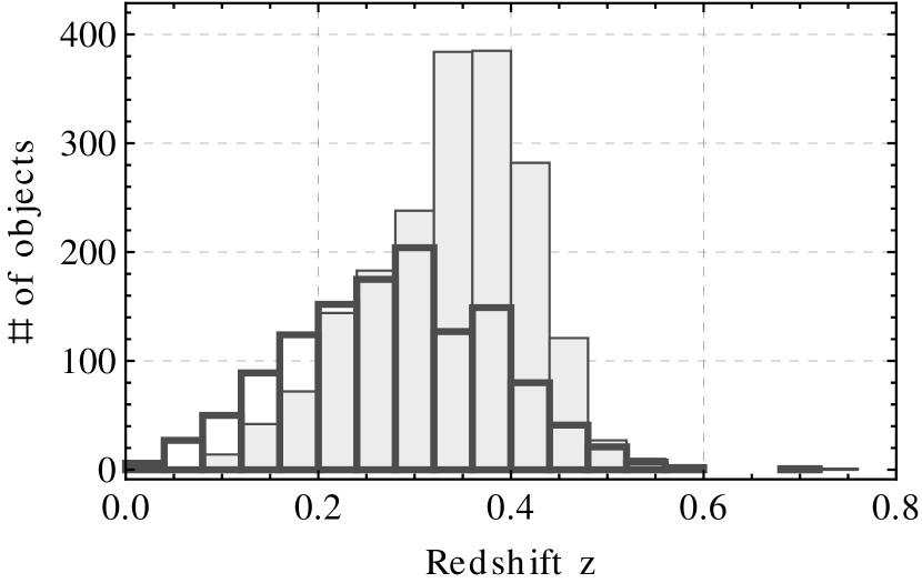
Figure 1: Histogram for the 1256 supernovae type Ia without any cuts (thick contours, no filling) and the 1905 GMBCG clusters (thin contours, gray filling) used in this paper.

2.3 Host galaxy photometry

The search for the SNe Ia’s host galaxy was done exclusively in the SDSS DR8 (Aihara et al., 2011) primary objects list, which includes the highest quality SDSS runs over the Stripe 82 region. Within the Stripe 82, approximately 5 million galaxies were detected. The evaluation of host galaxy properties was entirely photometric. When available, we supplemented SDSS DR8 photometry with ultraviolet and near infrared measurements taken by the Galaxy Evolution Explorer (GALEX, Martin et al., 2005) General Release 6 (GR6) and the UKIRT Infrared Deep Sky Survey (UKIDSS, Lawrence et al., 2007) Data Release 8 (DR8). GALEX has filters in far-UV and near-UV bands, while UKIDSS has filters in the YJHK bands (Hewett et al., 2006). We present our methods for identifying a SNIa’s host galaxy and for estimating its properties in section 3.2.

3 Methodology

3.1 SNIa model fitting

All supernovae type Ia were fitted using the SALT2 model (Guy et al., 2007) implemented by the publically available software snana (Kessler et al., 2009b). This SNIa light-curve model is based on five parameters: the redshift $z$, the time of maximum $T_{0}$, a overall normalisation $x_{0}$, a stretch or ‘light-curve width’ parameter $x_{1}$ and a colour parameter $c$. The normalisation $x_{0}$ is related to the apparent magnitude at peak in the B-band $m_{B}$ by:

$$m_{B}=10.635-2.5\log_{10}x_{0}\;.$$ (1)

The distance modulus $\mu\equiv 5\log_{10}(\frac{d_{\mathrm{L}}}{10\;\mathrm{pc}})$, where $d_{\mathrm{L}}$ is the luminosity distance, is calculated using corrections based on $x_{1}$ and $c$ that account for the fact that SNe Ia with wider light curves ($x_{1}>0$) tend to be brighter, and redder SNe Ia ($c>0$) tend to be dimmer:

$$\mu=m_{B}-M+\alpha x_{1}-\beta c\;.$$ (2)

In the equation above, $M$ (an average absolute magnitude), $\alpha$ and $\beta$ (often called ‘nuisance parameters’) are obtained from a sample of SNe Ia so that the $\chi^{2}$ for $\mu$ around the best-fit cosmology is minimized. When calculating $\chi^{2}$, in addition to the measurement errors, we included an intrinsic dispersion $\sigma_{\mathrm{int}}$ such that the minimum reduced $\chi^{2}$ is set to $\sim 1$, as commonly done by papers that use the SALT2 model (e.g. Sullivan et al., 2010; Lampeitl et al., 2010; Campbell et al., 2013).

For the determination of $\mu$, $M$, $\alpha$ and $\beta$ the software salt2mu in snana package was used (Marriner et al., 2011). While searching for the best $M$, $\alpha$ and $\beta$ values, instead of varying the cosmological density parameters for matter and dark energy ($\Omega_{m}$ and $\Omega_{\Lambda}$) or the dark energy equation of state, salt2mu uses a constant fiducial cosmological model and parametrizes deviations from it due to cosmology and other redshift dependent effects with different SNe Ia absolute magnitudes at different redshift ranges. Thus, even though we adopted throughout this work a fiducial flat $\mathrm{\Lambda CDM}$ cosmological model with $\Omega_{\mathrm{m}}=0.27$, $\Omega_{\mathrm{\Lambda}}=0.73$ and $H_{0}=70\;\mathrm{km\;s^{-1}\;Mpc^{-1}}$ (Kessler et al., 2009a), our nuisance parameters are not constrained by this particular model.

The Hubble residuals ($HR\equiv\mu_{\mathrm{SN}}-\mu_{z}$) are given by the difference between the distance modulus $\mu_{\mathrm{SN}}$ obtained from data via Eq. 2 and the expected distance modulus $\mu_{z}$ from our fiducial cosmology, thus they are the residuals after correction by colour and stretch.

After fitting the SNe Ia light curves, we removed 12 outliers from our 1122 SNe Ia based on their light curve properties: 9 with $|x_{1}|\geq 5$ and 3 extremely red SNe Ia with $c>0.45$. Furthermore, we excluded 37 SNe Ia whose SALT2 fit $\chi^{2}$ probability was smaller than 0.01. Lastly, we removed 10 outliers that were unusually off the Hubble diagram (more that 4$\sigma$), reducing our sample to 414 spectroscopically and 649 photometrically typed SNe Ia. Even for a large sample, these outliers alone can alter significantly the nuisance parameters and the intrinsic scatter, and we are interested in values that are representative of the whole sample.

3.2 Host galaxies

3.2.1 Identification of the host galaxy

The identification of a SNIa’s host galaxy was done by searching in the SDSS DR8 primary objects list for all galaxies within a 30 arcsec radius of the SNIa. We then selected as host the galaxy whose angular separation from the SNIa, normalised by the angular elliptical radius of the galaxy in the direction of the SNIa (called ‘directional light radius’), $d_{\mathrm{DLR}}$, was the smallest. To compute the elliptical radius we used the Petrosian half-light radius as a measure of the size of the galaxy and its Stokes parameters $Q$ and $U$ as a measure of its ellipticity and orientation, all in the $r$ band (Abazajian et al., 2009). When these parameters were unavailable the object in question was not considered a viable host. To avoid misidentifications we also imposed a maximum $d_{\mathrm{DLR}}$ of 4.

Of the 1063 SNe Ia selected in section 3.1, 1017 (96 per cent) have an associated host. More information about the host identification process is available on the SDSS-II Supernova Survey 3-Year Data Release paper (Sako et al., 2013, in prep.). A similar process of host identification was adopted in Sullivan et al. (2006).

3.2.2 Host galaxy properties

The host galaxy properties were estimated by fitting synthetic spectral energy distributions (SED) to the galaxy photometry obtained by the SDSS, GALEX and UKIDSS surveys. The matching among the surveys was done by selecting the object in UKIDSS and/or GALEX catalogues nearest (on the sky plane) to a SDSS galaxy, with a maximum angular separation of $5$ arcsec. Out of 1017 SNe Ia with identified SDSS host, 455 had matches in both GALEX and UKIDSS, 222 had a match only in UKIDSS, 239 only in GALEX and 101 had no matches in both catalogues. The magnitude measurements used were Model magnitudes for SDSS (Stoughton et al., 2002), Petrosian for UKIDSS and Kron-like elliptical aperture magnitude for GALEX (Petrosian, 1976; Kron, 1980). More information about our methods for combining photometry can be found in Gupta et al. (2011).

To generate the synthetic SEDs we used the Flexible Stellar Population Synthesis (FSPSv2.1) code (Conroy et al., 2009; Conroy & Gunn, 2010), with the same procedure as in Gupta et al. (2011) (with the sole difference in the cosmological parameters used). The basic inputs were the stellar spectral library BaSeL3.1 (Lejeune et al., 1997, 1998), the Padova stellar evolution model (Marigo & Girardi, 2007; Marigo et al., 2008), the Initial Mass Function (IMF) from Chabrier (2003) and the dust model from Charlot & Fall (2000). For more details, please refer to Conroy et al. (2009).

The SEDs were generated on a grid of four FSPS parameters: the time when star formation begins $t_{\mathrm{start}}$; a star formation rate (SFR) time scale $\tau_{\mathrm{SF}}$, where $\mathrm{SFR}(t)\propto e^{-t/\tau_{\mathrm{SF}}}$; the metallicity $\log(Z/Z_{\odot})$, assumed constant over time; and a coefficient $\tau_{\mathrm{dust}}$ for the optical depth $\tau(t)$ around the stars of age $t$, given by:

$$\tau(t)=\begin{cases}3\tau_{\mathrm{dust}}\left(\frac{\lambda}{5500\mathrm{\AA}}\right)^{-0.7}\,,&t\leq 10\;\mathrm{Myr}\,,\\ \tau_{\mathrm{dust}}\left(\frac{\lambda}{5500\mathrm{\AA}}\right)^{-0.7}\,,&t>10\;\mathrm{Myr\,.}\end{cases}$$ (3)

The model fluxes on the far-UV, near-UV, ugriz and YJHK bands were then calculated using these SEDs. The measured fluxes were corrected for galactic extinction using the Cardelli curve (Cardelli et al., 1989) and Milky Way dust maps (Schlegel et al., 1998), and the SDSS and UKIDSS magnitudes were corrected to the AB system using Kessler et al. (2009a) and Hewett et al. (2006), respectively. The best fit model was chosen by comparing these measured fluxes to the model fluxes using the least squares method. No requirements were made regarding the number of bands measured.

Three host galaxy properties were estimated from the fits: the stellar mass (amount of mass in the form of stars), the mass-weighted average age and the specific star formation rate (sSFR). The stellar mass was obtained by multiplying the de-reddened measured r band luminosity with the model mass-to-light ratio on the same band. The mass-weighted average age was calculated as:

$$\langle\mathrm{Age}\rangle=A-\frac{\int_{0}^{A}t\Psi(t)dt}{\int_{0}^{A}\Psi(t)dt}\,,$$ (4)

where $A$ is the age of the universe at the galaxy’s redshift minus $t_{\mathrm{start}}$ and $\Psi$ is the SFR. The sSFR was obtained by normalising $\Psi(t)$ over the period $A$ to unity, and taking the average over the interval $A-250\;\mathrm{Myr}<t<A$. To reduce the amount of noise in the host property analysis, we disconsidered hosts whose photometry fit presented a chi-square $p$-value smaller than 0.001. This reduced the number of available hosts from 1017 to 717, mainly due to the models in our grid being non-representative. Part of these exclusions may also be caused by matching the wrong objects through GALEX, UKIDSS and SDSS catalogues. A detailed description of the host galaxy’s properties estimation can be found in Gupta et al. (2011).

When necessary, we separated our hosts in two groups based on their sSFR ($\mathrm{sSFR}<-11.72$ are called ‘passive’ and $\mathrm{sSFR}>-10.5$, ‘active’). These sSFR limits were based on Lampeitl et al. (2010) – the -11.72 limit for passive galaxies is, on average, 1$\sigma$ below the active galaxies limit of -10.5 – and were chosen so the separation between these two classes is clean. 438 hosts galaxies were classified as active and 162 were classified as passive.

3.3 Selection of SNe Ia as members of clusters

With the purpose of classifying a SNIa as a member of a galaxy cluster we defined three criteria that should be fulfilled: their angular positions should be compatible, their redshifts should be compatible, and the cluster in the catalogue should be real and not a projection of field galaxies. For the last two criteria we adopted a probabilistic approach which combined them into a single condition described by Eq. 9. These criteria are described below in detail.

3.3.1 Selection of SNe Ia projected on clusters

In order to identify the SNe Ia that are inside SDSS GMBCG galaxy clusters, we started by selecting all supernovae type Ia within a projected $1.5\mathrm{Mpc}$ physical radius around any cluster, as done in previous studies of SNIa rate in galaxy clusters (see Mannucci et al., 2008; Dilday et al., 2010). For a given SNIa $s$ and a cluster $k$, this selection translates into obeying the following relation:

$$\cos\delta_{s}\cos\delta_{k}\cos\left(\alpha_{s}-\alpha_{k}\right)+\sin\delta_{s}\sin\delta_{k}\geq\cos\left(\theta_{\mathrm{max}}^{(k)}\right)\;,$$ (5)

$$\theta_{\mathrm{max}}^{(k)}\equiv\frac{1.5\mathrm{Mpc}(1+z_{k})}{c\int_{0}^{z_{k}}\frac{dz}{H(z)}}\;,$$ (6)

where $\theta_{\mathrm{max}}^{(k)}$ is the angular radius of the cluster $k$, $c$ is the speed of light, $\alpha_{s}$ and $\delta_{s}$ are the right ascension and declination of the SNIa, $\alpha_{k}$, $\delta_{k}$ and $z_{k}$ are the right ascension, declination and redshift of the cluster, respectively, and $H(z)$ is the Hubble parameter, given by:

$$H(z)=H_{0}\sqrt{\Omega_{\mathrm{m}}(1+z)^{3}+\Omega_{\mathrm{\Lambda}}}\;.$$ (7)

Of the 414 spectroscopically confirmed SNe Ia, 82 are projected onto clusters (21 of these on more than one); and of the 649 photometrically typed SNe Ia, 148 are projected, 32 being onto more than one cluster.

3.3.2 Redshift compatibility

The next step for determining if a SN belongs to a cluster was to check for redshift compatibility between the SN and the clusters onto which they were projected. Since galaxy clusters are gravitationally bound objects, there is no Hubble flow inside them, and if it were not for peculiar velocities of its members, all objects inside it would have the same redshift. Therefore, the tolerance on redshift difference between the supernova and the cluster arises from a combination of the velocity dispersion inside the cluster, which we assumed to be $\sigma_{v}=500$ $\mathrm{km\;s^{-1}}$, and measurement errors.

For each pair of cluster and projected SNIa we calculated the probability $p$ for their redshift difference to be inside a characteristic range. We assumed that the supernova and cluster redshift probability distribution were Gaussians $N(z_{s},\sigma_{s})$ and $N(z_{k},\sigma_{k})$, respectively, where $z_{s}$ and $\sigma_{s}$ ($z_{k}$ and $\sigma_{k}$) are the redshift assigned to the supernova (cluster) and its uncertainty. The probability distribution for the difference in redshift is then $N(z_{s}-z_{k},\;\sqrt{\sigma_{s}^{2}+\sigma_{k}^{2}})$, and the probability for compatible redshifts was calculated as:

$$p=\frac{1}{\sqrt{2\pi(\sigma_{s}^{2}+\sigma_{k}^{2})}}\int_{-z_{\mathrm{d}}}^{z_{\mathrm{d}}}e^{-\frac{[z-(z_{s}-z_{k})]^{2}}{2(\sigma_{s}^{2}+\sigma_{k}^{2})}}dz\;.$$ (8)

The choice of $z_{\mathrm{d}}$ depended on the type of redshift assigned to the cluster. For the 576 clusters with spectroscopically confirmed BCGs, the BCG spec-z was used, in which case the maximum redshift difference was $z_{\mathrm{d}}=0.005$, corresponding to a maximum velocity difference of $3\sigma_{v}=1500$ $\mathrm{km\;s^{-1}}$. For the 1329 remaining clusters with photometric redshifts only, the choice was $z_{\mathrm{d}}=0.030$. The process for choosing these values is described in Appendix A. No distinction was made on whether $z_{s}$ was the supernova’s redshift itself or its host galaxy’s redshift.

3.3.3 Cluster existence and final selection

For all clusters with SNe Ia projected onto them we calculated the probability $q$ of it being truly a cluster and not just a projection of field galaxies. We assumed that such probability is equal to the purity estimated by Hao et al. (2010) for the cluster catalogue in the redshift and richness range accessed by the cluster in question. These are presented in Table 1.

Table 1: Probability $q$ that a cluster in the redshift range given by the first column and in the richness range given by the first row is real. The values are based on the purity estimations made using mock catalogues.

	$r<15$	$15\leq r<20$	$20\leq r<25$	$r\geq 25$
$z<0.15$	0.78	0.96	1.00	0.99
$0.15<z<0.20$	0.70	0.92	0.98	0.98
$0.20<z<0.25$	0.70	0.89	0.98	0.98
$0.25<z<0.30$	0.55	0.82	0.92	0.96
$0.30<z<0.35$	0.48	0.81	0.91	0.95
$0.35<z<0.40$	0.62	0.89	0.92	0.98
$0.40<z<0.45$	0.51	0.84	0.93	0.94
$z>0.45$	0.78	0.90	0.90	0.97

The final step for selecting SNe Ia as cluster members was to pick from the projected ones those obeying the relation:

$$qp\geq P_{\mathrm{min}}\;,$$ (9)

where $P_{\mathrm{min}}=0.5$ is a minimum probability chosen through the procedure described in Appendix A. This equation states that a SNIa is only considered to be inside a cluster if the cluster is real and their redshifts are compatible. Assuming that these conditions are independent, the probability of fulfilling both criteria is equal to the product of $q$ and $p$.

After selecting for redshift compatibility with a real cluster, 6 (15) spectroscopically confirmed and 17 (10) photometrically typed SNe Ia were assigned to clusters with spectroscopic (photometric) redshifts, making a total of 48 cluster type Ia supernovae, which are presented in Table LABEL:tab:fulltable. As explained in Appendix A, the contamination by field SNe Ia was estimated as 29 per cent. The 1015 SNe Ia that did not pass this selection criteria were considered to be field SNe Ia. Since the small size of the cluster SNe Ia sample and its high contamination will dominate the noise during sample comparisons, more strict cuts on the field sample are unnecessary for our purposes. Table 2 summarises the number of SNe Ia obtained after each cut and cluster sample selection step were taken.

Table 2: Amount of SNe Ia selected in each step of the cluster sample formation and its sub-divisions by host galaxy type. The columns present, from left to right, the number of SNe Ia: spectroscopically typed; photometrically typed; total (sum of the two); and left outside the cluster sample (therefore, in the field sample). Apart from the last one, all lines are a sub-set of the previous one, and show the number of SNe that: were typed as Ias by psnid; passed light-curve cuts; were not known peculiars; had $|x_{1}|<5$ and $|c|<0.45$; their SALT2 fit $\chi^{2}$ probability was larger than 0.01; are not outliers in the Hubble residuals; are projected onto clusters; were selected as cluster members; has an identified host; its host fit passed the chi-square test; its host was classified as active; its host was classified as passive.

	Spec.	Phot.	Total	Field total
Initial	504	752	1256	–
LC cuts	451	679	1130	–
No peculiars	443	679	1122	–
$x_{1}$–$c$ cuts	439	671	1110	–
$P(\chi^{2})>0.01$	414	659	1073	–
$HR$ $4\sigma$ cut	414	649	1063	–
Projected	82	148	230	–
$qp\geq P_{\mathrm{min}}$	21	27	48	1015
w/ host	19	27	46	971
w/ host fit	11	21	32	685
Active	2	7	9	429
Passive	7	12	19	143

3.3.4 Selection crosschecks

We compared our supernova selection with the one done by Dilday et al. (2010) (hereafter, D10) using the maxBCG cluster catalogue (Koester et al., 2007). In this work we made use of BOSS redshifts for supernova hosts, an option not available for D10. This advantage drastically increased the number of SNe Ia with spectroscopic redshifts (by 652) and its precision, resulting in better typing and, in particular, better redshift comparison with galaxy clusters. Whereas the maxBCG cluster catalogue used the SDSS DR4 (Adelman-McCarthy et al., 2006) and only one colour to find the red sequence, GMBCG used DR7 and two colours, thereby increasing the redshift depth and the number of clusters detected in the Stripe 82 region from 492 to 1905. This changes are expected to make our cluster SNIa sample larger, and thus should include the majority of supernovae selected by D10. However, D10 only accounted for cluster contamination by field galaxy projections when calculating SNIa rates and not during SNIa selection. Furthermore, they did not eliminate outliers based on light-curve parameters. Therefore, a few D10 SNe Ia will be excluded by our method. The comparison can also be affected by differences in goal and methodology.

D10 found 27 SNe Ia in maxBCG clusters, 6 of which were not used in this work because of lack of spec-z or differences in the SN typing. Out of the remaining 21, 11 were also selected by our criteria, 2 would have been selected if we had not accounted for cluster catalogue contamination and 1 was eliminated because of its colour of $0.73\pm 0.07$. From the remaining 7, 2 did not have a projected GMBCG cluster, 3 were excluded because of differences in the cluster redshift, and 2 because of more restrictive requirements used for the redshift compatibility.

We found 37 cluster SNe Ia not selected by Dilday, 14 of which are beyond maxBCG redshift limit of 0.3. From the remaining 23, 6 had their redshifts measured only by BOSS, 8 were not projected onto a maxBCG cluster and 1 was projected on a cluster with a different redshift. The last 8 SNe Ia had compatible maxBCG clusters and the reasons why they were not included in D10 could not be traced. It is possible that they were eliminated as non-Ias or were excluded by data quality cuts. Since the majority of the differences between D10 sample and ours are due to SN typing and the cluster catalogue used, we considered our selection methods compatible.

Another consistency check for our cluster sample selection method was to compare its host galaxy properties with the ones obtained for the field sample (except for the redshift, no other host property was used during our selection). Galaxies inside clusters are expected to be older, more massive and to have less star formation. Figs. 2, 3 and 4 show that such expectancy is met, and a Kolmogorov–Smirnov test (K–S test, see Mood et al., 1974) indicated that the observed differences are significant: the probability that both samples were drawn from the same distribution was $1.7\times 10^{-3}$ for the mass, $8.1\times 10^{-4}$ for the hosts age and $8.3\times 10^{-6}$ for the sSFR. A comparison between the samples average properties is shown in Table 3 and also confirms the patterns we expected.

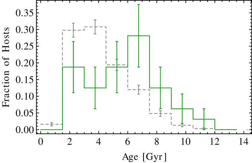
Figure 2: Histogram of the host galaxies mass-weighted average age for 32 cluster SNe Ia (green, solid line) and 685 field SNe Ia (gray, dashed line) that had good host fits. The cluster sample hosts are, on average, older than the hosts in the field sample.

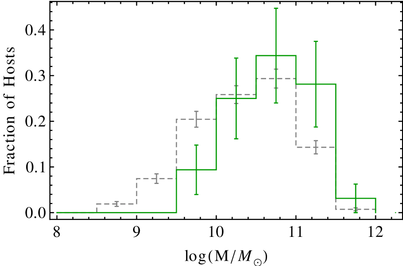
Figure 3: Histogram of the host galaxies stellar mass for 32 cluster SNe Ia (green, solid line) and 685 field SNe Ia (gray, dashed line) that had good host fits. The cluster sample host mass distribution is shifted to larger values.

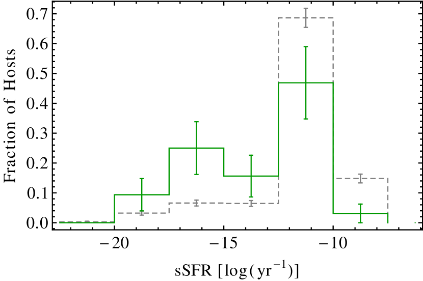
Figure 4: Histogram of the host galaxies specific star formation rate for 32 cluster SNe Ia (green, solid line) and 685 field SNe Ia (gray, dashed line) that had good host fits. Host galaxies in the cluster sample tend to present less star formation than those in the field sample.

Table 3: Average host properties for the subset of the cluster and field SNIa samples with good host fits (32 and 685 SNe Ia, respectively). The age, mass and specific star formation rate are given in Gyr, log of solar masses and log of mass fraction per year.

	Mean age	Mean mass	Mean sSFR
Cluster Sample	$5.82\pm 0.41$	$10.698\pm 0.087$	$-13.28\pm 0.52$
Field Sample	$4.22\pm 0.07$	$10.348\pm 0.023$	$-11.38\pm 0.11$
Difference	$1.60\pm 0.42$	$0.35\pm 0.09$	$-1.90\pm 0.53$

3.4 Comparing SNIa samples

To assess possible systematic differences between SNe Ia inside and outside galaxy clusters, we compared the $x_{1}$, $c$ and $HR$ distributions and their cross-correlations in both samples, along with their assigned $M$, $\alpha$, $\beta$ and $\sigma_{\mathrm{int}}$ parameters. The intrinsic scatter $\sigma_{\mathrm{int}}$ was obtained separately for each sample by making their Hubble residuals reduced $\chi^{2}$ go to $\sim 1$. For the $x_{1}$, $c$ and $HR$ distributions we computed their mean, median, standard deviation and median absolute deviation (MAD), which is defined for a sample $s=\{x_{1},x_{2},...,x_{N}\}$ as the median of $\{|x_{1}-x_{\mathrm{med}}|,|x_{2}-x_{\mathrm{med}}|,...,|x_{N}-x_{\mathrm{med}}|\}$ where $x_{\mathrm{med}}$ is the median of $s$. More attention was given to the median and MAD during the analysis since they are less sensitive to outliers.

To determine the significance of any difference observed on these properties, we used a resampling method of selecting from 5,000 to 20,000 random samples with the same size as the cluster sample from the combination of the field and cluster samples, and computing their properties. The fraction $P_{\mathrm{r}}$ of random samples presenting values equal to or more extreme than the ones obtained for cluster sample (known as $p$-value) yielded the probability that the difference observed is due to statistical fluctuations. In some cases, the SNIa set from which the random samples were drawn had a different composition. To avoid possible confusion, these cases are explained as they appear and its $P_{\mathrm{r}}$ are marked with special superscripts.

Differences in cross-correlations were assessed by fitting a linear model to the two parameters in question and comparing the line slope for both samples. The fitting was done minimising the $\chi^{2}$; this was accomplished after propagating the errors on the x-axis to the y-axis using a slope obtained from the data assuming equal weights to all data points. The significance of any slope difference was determined also by resampling.

We also searched for possible differences in correlations between SNIa parameters and host-galaxy properties – mass, age and specific star formation rate (sSFR) – using the same method described here. The errors for the host-galaxy parameters, especially sSFR and mass, are asymmetrical. In this case, the linear model fitting used an average of both errors.

4 Relations between SNe Ia and their host galaxies

To validate our methods and to have a basis for comparison when studying cluster SNIa properties, we first separated the SNe Ia by their host’s sSFR ($\mathrm{sSFR}<-11.72$ are called ‘passive’ and $\mathrm{sSFR}>-10.5$, ‘active’) and checked how reported relations between SNIa properties and that of their hosts appeared in our data. As mentioned in section 1, the best established reported relations between SNe Ia and their hosts are:

1. no clear difference in colour distribution was identified between SNe Ia in passive and active hosts;

2. SNe Ia in passive hosts have a faster-declining light-curve (smaller mean $x_{1}$);

3. the $\alpha$ parameter is the same regardless of the SNIa host;

4. the $\beta$ parameter for passive galaxies is lower than that for SNe Ia in active galaxies;

5. SNe Ia in passive galaxies are $\sim 0.1$ mag more luminous after corrections based on stretch and colour (their $M$ in Eq. 2 is more negative);

6. when fitted separately, SNe Ia in passive galaxies present less scatter on the Hubble residuals than SNe Ia in active galaxies.

When fitted with the same nuisance parameters, item 5 manifests itself through an offset on the Hubble diagram between the SNe Ia in passive and active galaxies, and through a correlation between Hubble residuals and host galaxy mass or age.

Figs. 5 and 6 show that while $c$ distributions for SNe Ia in passive and active galaxies do not present any significant differences, $x_{1}$ distributions are clearly different. A K–S test indicated that the probability that both $c$ samples are drawn from the same distribution is 0.47, while such probability is $3.4\times 10^{-12}$ for $x_{1}$. Table 4, however, presents some tension between the samples average colours, although this is not as significant as the difference in the average $x_{1}$. It is also possible to notice that the $x_{1}$ distribution in passive galaxies is significantly broader, a rarely reported result. It is in qualitative agreement with Smith et al. (2012, fig. 6), but in qualitative disagreement with Sullivan et al. (2006, fig. 12).

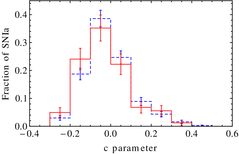
Figure 5: Histogram of the colour parameter $c$ distribution for SNe Ia in passive (solid red line) and active (blue dashed line) galaxies. Both histograms are consistent within the error bars.

Figure 6: Histogram of the stretch parameter $x_{1}$ distribution for SNe Ia in passive (solid red line) and active (blue dashed line) galaxies. The passive sample histogram is clearly shifted towards lower values of $x_{1}$. It also presents a larger scatter, probably due to its tails.

Table 4: Statistical measures for the $x_{1}$ and $c$ distributions of 162 and 438 SNe Ia in passive and active hosts. $P_{\mathrm{r}}^{\mathrm{*}}$ is the fraction of 20,000 random samples of SNe Ia in active galaxies, of same size as the passive sample, that present a value more extreme than the one observed for the passive sample.

$x_{1}$	Mean	Median	Std. Dev.	MAD
Passive	-0.328	-0.475	1.41	0.847
Active	0.382	0.381	1.18	0.695
$P_{\mathrm{r}}^{\mathrm{*}}$	$\la 5\times 10^{-5}$	$\la 5\times 10^{-5}$	$\la 5\times 10^{-5}$	0.001
$c$	Mean	Median	Std. Dev.	MAD
Passive	-0.0278	-0.0439	0.120	0.070
Active	-0.0135	-0.0294	0.117	0.066
$P_{\mathrm{r}}^{\mathrm{*}}$	0.027	0.024	0.320	0.217

When fitting for SNe Ia nuisance parameters separately in the passive and active sample, we obtained compatible values of $\alpha$ but significantly different values for $\beta$ and the average absolute magnitude $M$. Table 5 shows that our results are compatible with previously reported ones – items 3 to 5 above. The difference in Hubble residuals scatter, however, could not be detected. The MAD calculated for the active and passive sample were 0.167 and 0.152, with a probability $P_{\mathrm{r}}^{\mathrm{*}}$ for the active sample to reach the passive sample deviation of 0.241. A histogram of this distribution is shown in Fig. 7.

Table 5: Nuisance parameters, the Hubble residuals median absolute deviation $D_{\mathrm{HR}}$ and the intrinsic scatter obtained for the 162 and 438 SNe Ia in passive and active galaxies. $P_{\mathrm{r}}^{\mathrm{*}}$ was calculated from 5,000 random samples drawn from the active sample.

	$\alpha$	$\beta$	$M$	$D_{\mathrm{HR}}$	$\sigma_{\mathrm{int}}$
Active	0.180(18)	3.35(14)	-19.305(13)	0.167	0.17
Passive	0.206(20)	2.54(22)	-19.420(22)	0.152	0.16
$P_{\mathrm{r}}^{\mathrm{*}}$	0.229	$2\times 10^{-4}$	$\la 2\times 10^{-4}$	0.241	0.396

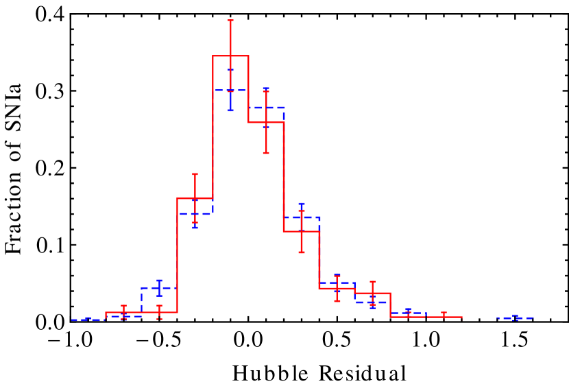
Figure 7: Histogram of the Hubble residuals for SNe Ia in passive (solid red line) and active (blue dashed line) galaxies obtained with each samples particular nuisance parameters. No clear difference can be noted.

The difference in the intrinsic scatter was not significant either, as Table 5 shows. This can also be noticed from Fig. 8, which presents the $\sigma_{\mathrm{int}}$ values obtained for the 5,000 randomly drawn samples of 162 SNe Ia hosted by active galaxies (the ‘active sample’). Given the large variability found for $\sigma_{\mathrm{int}}$ in these samples, even if the passive sample had a smaller value like $\sigma_{\mathrm{int}}=0.13$ (which could seem significant), it could still be achieved by 6.7 per cent of our active samples of same size.

The lack of detectable difference in the Hubble residuals scatter could be due to the exclusion of outliers through the 4$\sigma$ cut and to the use of the median absolute deviation instead of a standard deviation. In fact, when including the 10 outliers beyond 4$\sigma$ and comparing standard deviations, our active sample showed significantly larger scatter than the passive sample. However, we disregarded this result as it may be caused by non–Ia contamination.

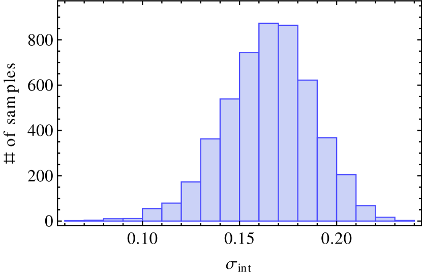
Figure 8: Histogram of the intrinsic scatter obtained for 5,000 randomly selected samples of 162 SNe Ia residing in active galaxies. For each random sample, $\sigma_{\mathrm{int}}$ was obtained by setting the minimum reduced chi-squared to $\sim 1$.

We compared our passive and active nuisance parameter values and intrinsic scatter with those obtained by Lampeitl et al. (2010) using the same resampling methodology. For instance, we selected, from our passive sample, 5,000 random samples containing 40 SNe Ia (same size as their passive sample) and counted the fraction that could reach their values. As Table 6 shows, all parameters were compatible for both samples.

Table 6: Nuisance parameters and intrinsic scatter obtained by Lampeitl et al. (2010) for a sample of 40 SNe Ia in passive hosts and 122 SNe Ia in active hosts, and the probability that our data could reach these values. $P_{\mathrm{r}}^{\mathrm{*}}$ was obtained from 5,000 random samples drawn from our active sample and $P_{\mathrm{r}}^{\mathrm{-}}$ was obtained from 5,000 random samples drawn from our passive sample. Their average magnitudes were corrected for the difference in the assumed $H_{0}$ and for the 10.635 offset between SALT2mu output and $B$ band AB magnitude.

	$\alpha$	$\beta$	$M$	$\sigma_{\mathrm{int}}$
Lampeitl’s Active	0.12(01)	3.09(10)	-19.30(01)	0.17
$P_{\mathrm{r}}^{\mathrm{*}}$	0.071	0.162	0.480	0.258
Lampeitl’s Passive	0.16(02)	2.42(16)	-19.39(03)	0.13
$P_{\mathrm{r}}^{\mathrm{-}}$	0.119	0.340	0.286	0.483

5 Cluster SNe Ia properties

5.1 Comparison with field sample

When comparing SNe Ia inside and outside rich galaxy clusters, no significant difference was found in the colour distribution (see Fig. 9 and Table 7). A K–S test, which returned a $p$-value of 0.74, did not indicate any differences either. However, there are several indications that the $x_{1}$ distribution in cluster SNe Ia differs from that of the field SNe Ia. A probability of 0.0021 was obtained from a K–S test with the null hypothesis that the two samples were drawn from the same distribution, and Table 7 shows that the cluster $x_{1}$ distribution is shifted to lower values. Furthermore, Fig. 10 suggests that the cluster sample $x_{1}$ distribution is bimodal, with the left peak consisting of mostly SNe Ia in passive hosts and the right peak consisting of mostly SNe Ia in active hosts. At least part of the SNe Ia in the right peak are actually contamination from the field, which has a high concentration of active galaxies ($\sim 63$ per cent in our sample).

The position of the left peak in Fig. 10, however, does not coincide with the position obtained for the passive sample depicted in Fig. 6: it is slightly more negative. To assess the significance of this difference, we compared the statistical properties of SNe Ia in passive hosts selected as being inside clusters with the full passive sample (see Fig. 11). The mean and median $x_{1}$ obtained for the former sample were -0.82 and -1.12, and the fraction of random samples of same size (19 SNe Ia) drawn from the full passive sample which could reach lower values were 0.05 and 0.006, respectively. This result indicates that the cluster environment may intensify the passive bias towards fast-declining SNe Ia, possibly by preferentially selecting very old hosts. This is investigated in section 5.3. A similar comparison was performed for the $x_{1}$ distribution of SNe Ia in active galaxies, but no significant difference was found.

Figure 9: Histogram of the SALT2 colour parameter for SNe Ia inside galaxy clusters (solid green line) and outside (gray dashed line). No significant difference is seen.

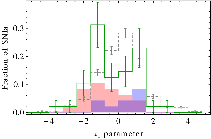
Figure 10: Histogram of the SALT2 stretch parameter for SNe Ia inside galaxy clusters (solid green line) and outside (gray dashed line). The difference between the distributions is significant and our cluster sample is bimodal in $x_{1}$. The red and blue shaded histograms present the cluster SNe Ia that had hosts typed as passive and active, respectively (their overlap is depicted in purple). Each shaded histogram is associated with a different cluster sample peak.

Table 7: Statistical measures for the $x_{1}$ and $c$ distributions of the 48 SNe Ia inside and 1015 outside clusters. $P_{\mathrm{r}}$ was obtained from 20,000 random samples.

$x_{1}$	Mean	Median	Std. Dev.	MAD
Field	0.142	0.202	1.27	0.763
Cluster	-0.398	-0.602	1.38	0.940
$P_{\mathrm{r}}$	$1.9\times 10^{-3}$	$2\times 10^{-4}$	0.232	0.104
$c$	Mean	Median	Std. Dev.	MAD
Field	-0.0113	-0.0270	0.121	0.069
Cluster	-0.0251	-0.0360	0.113	0.073
$P_{\mathrm{r}}$	0.218	0.301	0.311	0.332

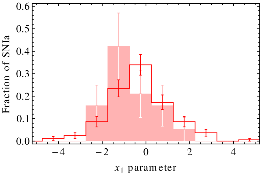
Figure 11: Comparison between $x_{1}$ distributions of the full passive sample (red contour, no filling) and the sub-sample of SNe Ia in passive galaxies inside rich galaxy clusters (no contour, red filling). The peak of the cluster histogram is shifted towards lower values of $x_{1}$.

For the nuisance parameters, Hubble residuals and intrinsic scatter, no significant difference could be identified between the cluster and the field sample, although $\beta$, $M$, $\sigma_{\mathrm{int}}$ and the Hubble residuals scatter follow the same trend as the full passive sample relative to the full active sample. As Table 8 shows, the probability $P_{\mathrm{r}}$ was fairly high for every parameter.

Table 8: Nuisance parameters, Hubble residuals median absolute deviation $D_{\mathrm{HR}}$ and the intrinsic scatter obtained for the cluster and field samples (containing 48 and 1070 SNe Ia, respectively). The quantity $P_{\mathrm{r}}$ was obtained from 5,000 random samples.

	$\alpha$	$\beta$	$M$	$D_{\mathrm{HR}}$	$\sigma_{\mathrm{int}}$
Field	0.180(09)	3.26(08)	-19.337(08)	0.155	0.16
Clusters	0.156(22)	2.46(32)	-19.389(30)	0.115	0.13
$P_{\mathrm{r}}$	0.320	0.085	0.129	0.104	0.556

Due to the small size of the sample (see Table 2), we did not perform a nuisance parameters fit for the sub-sample of SNe Ia in passive hosts in rich clusters. Such fits involve many parameters and thus the uncertainties would be quite large. We instead fitted for the whole passive sample and compared the mean values of the Hubble residuals for the SNe Ia belonging to clusters and to the field. Although the cluster sub-sample shows an offset from the field sub-sample of $-0.084$, 10 per cent of randomly selected samples of SNe Ia in passive hosts were able to mimic such difference. A larger cluster sample is necessary to determine if such offset is significant.

5.2 Comparison with mixed samples

Given that SNe Ia in passive and active hosts are known to differ, it is important to test if the cluster sample properties can be mimicked by samples with the same fraction of passive and active hosts, which we call ‘mixed samples’. Since 4.2 per cent of all SNe Ia did not have an identified host and 30.4 per cent of the remaining ones had hosts with bad fits, the composition of the cluster sample is not known precisely. Based on the fitted hosts, we estimated that the cluster sample should be composed of approximately 65 per cent passive and 35 per cent active hosts.

Comparisons were made to samples with a range of compositions, from 50 to 100 per cent of passive hosts. In all comparisons, the colour distribution and the nuisance parameters from both samples were compatible, while the $x_{1}$ distribution for the cluster sample had a mean and median value lower than every mixed sample. Since a higher fraction of passive hosts shifts the $x_{1}$ distribution to lower values, the compatibility of the $x_{1}$ distributions continually increases with the fraction of passive hosts in the mixed sample. As Table 9 and Fig. 12 show, it is unlikely that a mixed sample with a similar composition as the cluster sample could reach such a low value for the $x_{1}$ median. Ignoring the composition estimate for the cluster sample, it would be most compatible with the pure passive sample. An intermediate sample composition would probably be a better choice to explain the cluster sample. However, in section 6.4 we show that for SNe Ia closer to the cluster’s centre the difference in $x_{1}$ is significant even for samples with high passive host content.

Table 9: Average values obtained from 5,000 mixed samples composed by 70 per cent of passive and 30 per cent of active hosts (leftmost columns) and from 5,000 mixed samples composed by 100 per cent of passive hosts (rightmost columns). $P_{\mathrm{r}}^{70}$ and $P_{\mathrm{r}}^{-}$ give their respective fractions that could reach the cluster sample’s values.

0.7 passive	Value	$P_{\mathrm{r}}^{70}$	1.0 passive	Value	$P_{\mathrm{r}}^{-}$
$\alpha$	0.194	0.193	$\alpha$	0.221	0.072
$\beta$	2.88	0.224	$\beta$	2.64	0.355
$M$	-19.37	0.386	$M$	-19.43	0.215
HR MAD	0.16	0.049	HR MAD	0.16	0.038
$\sigma_{\mathrm{int}}$	0.13	0.446	$\sigma_{\mathrm{int}}$	0.12	0.488
$c$ median	-0.040	0.393	$c$ median	-0.042	0.426
$c$ MAD	0.067	0.279	$c$ MAD	0.069	0.344
$x_{1}$ median	-0.179	0.019	$x_{1}$ median	-0.458	0.241
$x_{1}$ MAD	0.86	0.241	$x_{1}$ MAD	0.80	0.129

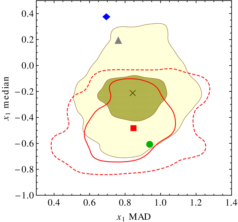
Figure 12: Comparison between samples $x_{1}$ median and MAD. The blue diamond and red square represent the active and passive samples, and the gray triangle and the green circle represent the field and cluster samples, respectively. The shaded regions represent the parameter space populated by 68 (dark shade) and 95 (light shade) per cent of the randomly selected mixed samples containing 70 per cent of passive hosts, and the cross indicate their mean value. The red contours represent the region populated by 68 (solid line) and 95 per cent (dashed line) of randomly selected samples from the passive sample. All random samples contain 48 SNe Ia. The cluster sample is barely consistent with samples with 70 per cent of passive hosts. A higher passive fraction is preferred.

5.3 The role of the host age

The relationship between galaxy age and environment density is a well established fact: passive galaxies in high-density regions – such as rich clusters – are, on average, $\sim 2$ Gyr older than passive galaxies in low-density regions, as shown by Thomas et al. (2005) using spectra of 54 early-type galaxies in high-density and 70 in low-density environments. Based only in our photometric data, we searched for age differences between passive galaxies inside and outside rich clusters, and Figure 13 shows that the cluster sample passive hosts were estimated to be, on average, older than the field passive hosts. However, the significance of such result is low since a K–S test returned a $p$-value of 0.157. Moreover, by resampling 20,000 times from the passive sample, we obtained 1206 (6 per cent) samples that could reach an average age higher than the cluster sample. The lack of significance in this detection is probably due to larger errors in the classification of galaxies and in the determination of their ages.

Figure 13: Comparison between host age distributions of the full passive sample (red contour, no filling) and the sub-sample of SNe Ia in passive galaxies inside rich galaxy clusters (no contour, red filling). The distribution for the cluster sample is shifted to larger values, although its significance is low.

The indication that passive galaxies inside rich clusters may host SNe Ia with smaller stretch than passive galaxies outside clusters prompted us to study possible causes for such difference. First of all, significant trends between SNIa stretch and host age have been reported by Gupta et al. (2011), that showed that older galaxies host SNe Ia with smaller $x_{1}$. While this result may be attributed to the differences presented in section 4 (since older galaxies are usually passive), such trend seems to remain within passive galaxies: Gallagher et al. (2008) have pointed out that early-type galaxies older than 5 Gyr host SNe Ia that are $\sim 1$ mag fainter than those in younger early-type galaxies. This result means that the stretch of SNe Ia in old passive galaxies should populate lower values than those in young passive galaxies. This conclusion was confirmed by our passive sample, as Fig. 14 shows. While the difference is still significant for the age cut of 5 Gyr proposed by Gallagher et al. (2008), our results are stronger using a separation at 8 Gyr, which created samples containing 132 (host age $<8$ Gyr, called ‘young’) and 30 (host age $>8$ Gyr, called ‘old’) SNe Ia. A K–S test between SNe Ia $x_{1}$ distribution in young and old passive galaxies returned a $p$–value of $3.4\times 10^{-5}$.

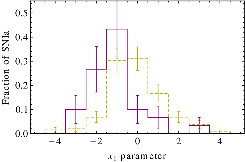
Figure 14: Comparison between $x_{1}$ distributions of SNe Ia hosted by old ($>8$ Gyr) passive galaxies (solid purple line) and of SNe Ia hosted by young ($<8$ Gyr) passive galaxies (dashed yellow line). SNe Ia in old passive galaxies have, on average, a smaller stretch than those in young passive galaxies.

5.4 Correlation with host galaxy mass

Many authors have shown the correlation between SNIa Hubble residuals and their host galaxy’s mass (e.g. Gupta et al., 2011; Lampeitl et al., 2010). Fig. 15 presents the correlation obtained for our sample of field and cluster SNe Ia; both groups present this same trend and they are compatible, since a probability $P_{\mathrm{r}}$ for the cluster sample slope was calculated at 7.5 per cent, not a high significance level.

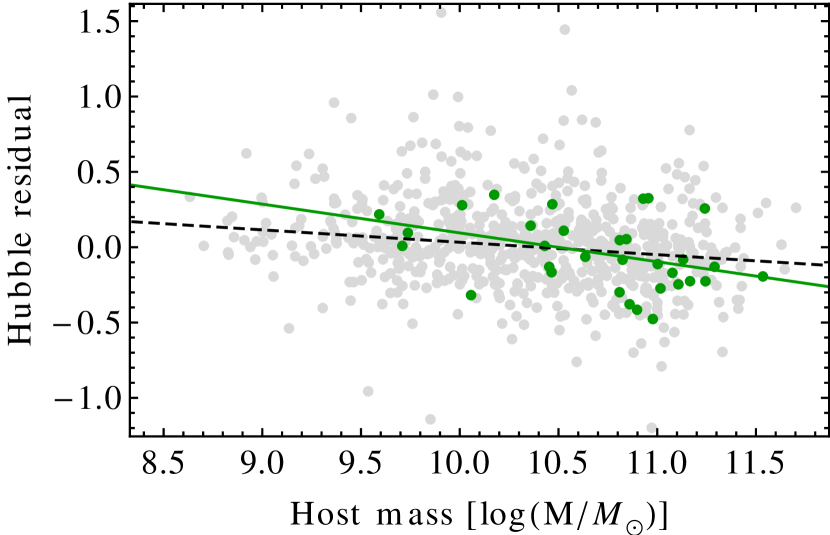
Figure 15: Correlation between SNIa Hubble residuals and its host mass for the field (gray dots) and cluster (green dots) samples. The black dashed and green solid lines are linear fits adjusted to the field and cluster samples, with slopes $-0.082\pm 0.015$ and $-0.191\pm 0.078$, respectively. Both samples show anti-correlations that are compatible at 7.5 per cent. The errors bars were hidden to facilitate visualisation.

6 Robustness tests

To verify how our conclusions depend on our methods, we tested how the use of stringent cuts on $x_{1}$ and $c$ parameters, the cluster sample redshift distribution, the assumed cluster radius and the host galaxy photometry used could affect our findings.

6.1 $x_{1}$ and $c$ cuts

To test whether our results depend on the core or on the tails of SNe Ia distributions in $x_{1}$ and $c$ and to further remove contamination by non–Ia SNe, we repeated our analysis after applying the elliptical cut suggested by Campbell et al. (2013). This cut – presented in Fig. 16 – was chosen through simulations and is expected to remove a larger fraction of non–Ia than of Ia SNe. Table 10 presents the sample sizes after this cut.

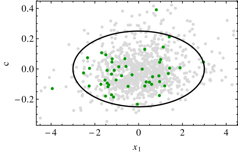
Figure 16: Distribution of SNe Ia on the $x_{1}$–$c$ parameter space and the region chosen to be analysed separately (black line). The ellipse is centred in ($x_{1}=0,c=0$) and has semi-major axis $a_{x_{1}}=3$ and semi-minor axis $a_{c}=0.25$. The gray and green dots represent field and cluster SNe Ia, respectively.

Table 10: Amount of SNe Ia in the cluster and field samples after selecting those inside the ellipse depicted in Fig. 16.

	SNe Ia	w/ host fit	Active	Passive
Cluster	45	30	8	19
Field	896	602	385	122

This cut did not affect any of our conclusions since the significance of the parameters difference did not change much. One more subtle result was the comparison between the passive and active samples $x_{1}$ distribution width. After the cut, this difference was only noticeable in the distribution’s standard deviation, as $P_{\mathrm{r}}^{*}$ for the MAD got to 0.199. This result corroborates the hypothesis that the passive sample include some extra SNe Ia on its $x_{1}$ distribution’s tails, but which are still present in the $-3\la x_{1}\la 3$ range.

When comparing the full passive sample with its sub-sample residing in rich clusters, the significance of the difference between the $x_{1}$ mean and median values was slightly strengthened: the fractions $P_{\mathrm{r}}^{-}$ of random samples drawn from SNe Ia in passive galaxies that could surpass the cluster sub-samples $x_{1}$ mean and median were 0.011 and 0.002, indicating that such difference is not caused by non–Ia contamination. All other $x_{1}$ comparisons maintained similar significance levels.

6.2 Redshift dependence

Even though the redshift distribution of the cluster and field samples are not very different, we checked if our results could be caused by redshift selection. For that we counted the number of cluster SNe Ia in 0.05 wide redshift bins and randomly selected the same number of SNe Ia in each bin from our full sample, creating 5,000 random samples with same size and redshift distribution as the cluster sample, which we called ‘same–z samples’. Our significance analysis was then repeated using these samples.

All the results from section 5.1 were reobtained at very similar significance levels. We did not perform this test for the comparison between the cluster sample and the mixed samples since the passive sample is not big enough to adequately sample the parameter space after being broken into bins of redshift.

As a consistency check, we also looked for possible differences between the same–z samples and the original full sample. Not a single property was found to differ significantly, as for all of them, at least 10 per cent of the same–z samples were able to achieve the full sample values. This test shows that the effect of redshift selection is unlikely to cause the differences we observed.

6.3 Only optical photometry

Since combining host galaxy photometry from different surveys might cause a few problems like matching wrong objects across the catalogues and small differences in the magnitude aperture and calibration, we also performed our analysis using host properties obtained from the SDSS photometry alone. The effects of excluding GALEX and UKIDSS from the galaxy properties determination was investigated in Gupta et al. (2011) and in general it increases the errors for all host parameters, specially for sSFR. In addition, it compresses the estimated ages to a smaller range centred around 6 Gyr. Such effects were also verified in this work. The elimination of GALEX and UKIDSS photometry can only affect analysis involving host galaxy properties, therefore all conclusions regarding the differences between the field and cluster samples remains unaltered.

While the significance levels of our results changed when using SDSS photometry only, these changes were small and, for most cases, did not affect our conclusions. All differences between the active and passive sample remained significant, as well as the difference in the $x_{1}$ distribution for SNe Ia in old and young passive galaxies. The difference in $x_{1}$ median between the cluster (using the maximum separation of 1.5 Mpc) and the mixed samples, however, lost its significance since the fraction of mixed samples with 70 per cent passive hosts that could surpass the cluster sample $x_{1}$ median was 0.07. This result is, therefore, dependent on the use of GALEX and UKIDSS photometry. When comparing the sample closer to the cluster core (within 1.0 Mpc from the centre – see section 6.4) to the mixed samples, the significance of this difference remained.

6.4 Cluster radius

We repeated our analysis using a physical radius of 1.0 Mpc during the projection test described in section 3.3.1, which reduced the cluster sample to 31 SNe Ia. This change can only affect analysis involving the cluster sample, thus comparisons between the active and passive sample and between SNe Ia inside old and young passive galaxies were not affected. Most of the results related to the cluster sample were consistent with the ones obtained using 1.5 Mpc. Few exceptions appeared in the form of an intensification of previous signals, which may indicate that some contamination from the field can be eliminated with a smaller radius, or that SNe Ia closer to the core of clusters are the ones responsible for the differences seen between the field and cluster samples. It is important to note that, with the reduction of the radius, the estimated fraction of passive galaxies increase to approximately 75 per cent. This corroborates our conclusion that the SNe Ia responsible for the differences observed reside in passive galaxies. Moreover, the strengthening of previous signals presented in this section qualitatively agrees with the connection between host age and SNe Ia properties presented in section 5.3, since older galaxies are expected to populate the inner, denser regions of clusters (Balogh et al., 1999; Thomas et al., 2005).

The cluster sample $x_{1}$ distribution got shifted to smaller values, increasing the difference when compared to the field and mixed samples. Its mean and median got to -0.75 and -1.12, respectively, and the probability $P_{\mathrm{r}}$ for getting this same result from the full SNe Ia sample was $10^{-4}$ for the mean and less than that for the median. When comparing with the full passive sample, $P_{\mathrm{r}}$ was calculated as 0.026 for the $x_{1}$ mean and $6\times 10^{-4}$ for the $x_{1}$ median. Table 11 compares the values obtained for the 1.5 and the 1.0 Mpc cluster radius and their probabilities $P_{\mathrm{r}}$ and $P_{\mathrm{r}}^{-}$ for drawing these values from the full and the passive samples, respectively.

Table 11: Mean and median SALT2 parameters $x_{1}$ and $c$ obtained for the field sample, the passive sample, and the cluster sample using 1.5 and 1.0 Mpc physical radius during the projection test described in section 3.3.1. Following each cluster sample values, we present the probabilities $P_{\mathrm{r}}$ and $P_{\mathrm{r}}^{-}$ that a more extreme value could be reached by random selections from the full SNe Ia sample and the passive sample.

	$x_{1}$ mean	$x_{1}$ median	$c$ mean	$c$ median
Field	0.142	0.202	-0.0113	-0.0270
Passive	-0.328	-0.475	-0.0278	-0.0439
1.5 Mpc	-0.398	-0.602	-0.0251	-0.0360
$P_{\mathrm{r}}$	$1.9\times 10^{-3}$	$2\times 10^{-4}$	0.218	0.301
$P_{\mathrm{r}}^{-}$	0.347	0.241	0.426	0.347
1.0 Mpc	-0.750	-1.118	-0.0410	-0.0454
$P_{\mathrm{r}}$	$10^{-4}$	$\la 10^{-4}$	0.081	0.224
$P_{\mathrm{r}}^{-}$	0.026	$6\times 10^{-4}$	0.246	0.431

7 Conclusions and summary

We used SDSS photometrically and spectroscopically typed SNe Ia, galaxy photometry from SDSS, GALEX and UKIDSS, and the GMBCG optical cluster catalogue to study the properties of SNe Ia residing in rich galaxy clusters. Their light curves were parametrized by the SALT2 model.

To test our samples and methods, we first analysed the properties of SNe Ia residing in active and passive galaxy hosts and compared our results to the literature (see section 4). We confirm previously reported differences between these SNe Ia, namely that passive galaxies host SNe Ia that: (a) have smaller average $x_{1}$ (see Fig. 6); (b) are $\sim 0.1$ mag brighter after corrections based on $x_{1}$ and $c$; and (c) have a smaller SALT2 $\beta$ parameter. Moreover, (d) the consistency between SALT2 $\alpha$ parameters obtained for SNe Ia in active and passive galaxies was also confirmed. Contrary to previous works, we (e) could not detect a significant difference in the Hubble residual scatter: even though the Hubble residual intrinsic scatter and median absolute deviation were smaller in passive galaxies, they were considered consistent with those obtained for SNe Ia in active galaxies. This indicates that any differences that might be observed are due to a few objects in the active sample that present high dispersion. Items (b) through (e) are summarised in Table 5. We also report that the $x_{1}$ distribution of our passive sample is significantly broader than that of our active sample (see Table 4).

We then analysed SNe Ia residing in rich galaxy clusters, and concluded that their SALT2 $x_{1}$ distribution is different from that of their counterparts in the field (see Fig. 10 and Table 7): it is shifted to lower values, and the probability that a lower median could be obtained from a randomly selected SNe Ia sample was estimated as $2\times 10^{-4}$. Although this could be explained by a higher content of passive galaxies SNe Ia than the estimated one (of 65 per cent, see section 5.2), this explanation is not sufficient for regions closer to the core of the cluster (see section 6.4). Moreover, we found evidence that passive galaxies inside rich clusters may host SNe Ia with smaller $x_{1}$ than passive galaxies outside them (see Fig. 11). This difference could be due to a higher content of old passive galaxies in clusters as shown by Thomas et al. (2005). As demonstrated in section 5.3, old passive galaxies host SNe Ia with smaller $x_{1}$ than young passive galaxies (see Fig. 14), a result compatible with the findings by Gallagher et al. (2008).

Other cluster SNe Ia parameters – their colour distribution, nuisance parameters and Hubble residual scatter – were found to be consistent with those of field SNe Ia, although they all followed the same trends as SNe Ia in passive galaxies do when compared to SNe Ia in active galaxies. To verify if differences exist in these parameters, larger samples are required. Current and near-future projects like DES, Pan-STARRS and J-PAS are expected to increase the SNIa sample sizes by a factor of 5 or more. The combination of the SDSS dataset with other datasets, provided these overlap with a cluster catalogue, would also increase sample sizes. However, this combination might encounter difficulties due to possible systematic differences between the datasets. An interesting possibility to better constrain these results would be to assess host properties using spectroscopy, which exists for all SNe Ia used here, thanks to the BOSS project.

Appendix A Determining sample requirements

A.1 Derivation of a guiding formula

When deciding the requirements SNe Ia must fulfill in order to be considered members of galaxy clusters, one must face a trade-off between completeness and purity. Highly restrictive requirements will result in a small but pure sample, while low requirements will result in a large but contaminated sample. In order to guide our decision on the best type of sample to address our problem, suppose that some SNIa property $X$ has the average value $\bar{X}_{S}$ for SNe Ia in one sample $S$ and $\bar{X}_{S^{\prime}}$ in a different sample $S^{\prime}$. One way to determine if $S$ and $S^{\prime}$ have distinct properties is by applying a difference test such as the Z-test (Sprinthall, 1990):

$$Z=\frac{\bar{X}_{S}-\bar{X}_{S^{\prime}}}{\sqrt{\sigma_{\bar{X}_{S}}^{2}+\sigma_{\bar{X}_{S^{\prime}}}^{2}}}\;,$$ (10)

where $\sigma_{\bar{X}_{S}}^{2}$ and $\sigma_{\bar{X}_{S^{\prime}}}^{2}$ are the variances of the mean of $X$ for the $S$ and $S^{\prime}$ sample. High $Z$ values indicate that the samples in question represent different populations.

Now consider that sample $S$ ($S^{\prime}$) contains $N_{S}=N_{\mathrm{C}}+N_{\mathrm{F}}$ ($N_{S^{\prime}}=N_{\mathrm{C}}^{\prime}+N_{\mathrm{F}}^{\prime}$) SNe Ia, where $N_{\mathrm{C}}$ ($N_{\mathrm{C}}^{\prime}$) supernovae are actually in clusters and $N_{\mathrm{F}}$ ($N_{\mathrm{F}}^{\prime}$) are in field galaxies. Assuming that the variances for the cluster and the field population are the same ($\sigma_{X_{\mathrm{C}}}^{2}=\sigma_{X_{\mathrm{F}}}^{2}=\sigma_{X}^{2}$), that

$$\sigma_{\bar{X}_{S}}^{2}=\frac{\sigma_{X_{S}}^{2}}{N_{S}}=\frac{\sum_{i=1}^{N_{S}}(X_{i}-\bar{X}_{S})^{2}}{N_{S}(N_{S}-1)}\simeq\frac{\bar{X^{2}}_{S}-\bar{X}_{S}^{2}}{N_{S}}\;,$$ (11)

and that

$$\bar{X}_{S}\simeq \frac{N_{\mathrm{C}}\bar{X}_{\mathrm{C}}+N_{\mathrm{F}}\bar{X}_{\mathrm{F}}}{N_{S}}\;,$$ (12)

$$\bar{X}_{S^{\prime}}\simeq \frac{N_{\mathrm{C}}^{\prime}\bar{X}_{\mathrm{C}}+N_{\mathrm{F}}^{\prime}\bar{X}_{\mathrm{F}}}{N_{S^{\prime}}}\;,$$

$$\bar{X^{2}}_{S}\simeq \frac{N_{\mathrm{C}}\bar{X^{2}}_{\mathrm{C}}+N_{\mathrm{F}}\bar{X^{2}}_{\mathrm{F}}}{N_{S}}\;,$$

$$\bar{X^{2}}_{S^{\prime}}\simeq \frac{N_{\mathrm{C}}^{\prime}\bar{X^{2}}_{\mathrm{C}}+N_{\mathrm{F}}^{\prime}\bar{X^{2}}_{\mathrm{F}}}{N_{S^{\prime}}}\;,$$

where $\bar{X}_{\mathrm{C}}$, $\bar{X^{2}}_{\mathrm{C}}$, $\bar{X}_{\mathrm{F}}$ and $\bar{X^{2}}_{\mathrm{F}}$ are the true $X$ and $X^{2}$ average values for the cluster and field populations, we arrive at the formula:

$$Z\simeq\frac{(1-\phi_{S}-\phi_{S^{\prime}})}{\sqrt{\frac{1}{N_{S}}+\frac{1}{N_{S^{\prime}}}+\delta^{2}\left[\frac{\phi_{S}(1-\phi_{S})}{N_{S}}+\frac{\phi_{S^{\prime}}(1-\phi_{S^{\prime}})}{N_{S^{\prime}}}\right]}}\delta\;,$$ (13)

$$\delta\equiv\frac{\bar{X}_{\mathrm{C}}-\bar{X}_{\mathrm{F}}}{\sigma_{X}}\;,$$ (14)

where $\phi_{S}\equiv\frac{N_{\mathrm{F}}}{N_{S}}$ and $\phi_{S^{\prime}}\equiv\frac{N_{\mathrm{C}}^{\prime}}{N_{S^{\prime}}}$. If we try to construct $S$ ($S^{\prime}$) mainly from cluster (field) SNe Ia, $\phi_{S}$ ($\phi_{S^{\prime}}$) is interpreted as a contamination fraction by field (cluster) supernovae. In our case, our tentative cluster SNIa sample $S$ will dominate both contamination and Poisson noise since $N_{S}\ll N_{S^{\prime}}$ and cluster SNIa is a rarer event than field SNIa. We then approximate Eq. 13 to:

$$Z\simeq\frac{(1-\phi_{S})\sqrt{N_{S}}}{\sqrt{1+\phi_{S}(1-\phi_{S})\delta^{2}}}\delta\;.$$ (15)

For a given $\delta$, we must find the sample $S$ membership requirements (in this work, the maximum angular separation $\theta_{\mathrm{max}}^{(k)}$, maximum redshift difference $z_{\mathrm{d}}$ and minimum probability of compatible redshift with a true cluster $P_{\mathrm{min}}$) which maximize $Z$. To accomplish this task, we must estimate how the requirements influences the contamination $\phi_{S}$.

A.2 Estimating sample contamination

For clusters with spectroscopic redshifts

The choice of $\theta_{\mathrm{max}}^{(k)}$ was based on previous studies (see Dilday et al., 2010; Mannucci et al., 2008) and set to a maximum projected physical separation of 1.5 Mpc. In this work we did not assess how the choice of $\theta_{\mathrm{max}}^{(k)}$ affected the contamination, and assumed that SNe Ia within this angular separation are necessarily projected onto the cluster. The maximum redshift difference $z_{\mathrm{d}}$ for clusters with spec-z was set to $0.005$, corresponding to a 1500 $\mathrm{km\;s^{-1}}$ maximum difference in cluster member velocities. For a Gaussian velocity dispersion with $\sigma_{v}=500\mathrm{km\;s^{-1}}$, this corresponds to a maximum difference of $3\sigma_{v}$.

The contamination of our cluster SNIa sample by field SNe Ia, $\phi_{S}$, was calculated as:

$$\phi_{S}=\sum_{n=1}^{N_{S}}\left[(1-q_{n})+q_{n}(1-p_{n})+q_{n}p_{n}\Pi_{n}\right]\;,$$ (16)

where $q_{n}$ is the probability given by Table 1 that the cluster onto which the supernova $n$ is projected is real, $p_{n}$ is the probability that the supernovae $n$ belonging the the sample $S$ has a compatible redshift with the cluster, obtained by Eq. 8. Every SNIa in this sample must have $q_{n}p_{n}>P_{\mathrm{min}}$ (besides a angular separation less than $\theta_{\mathrm{max}}^{(k)}$); thus $P_{\mathrm{min}}$ controls both $N_{S}$ and $\phi_{S}$.

The $q_{n}p_{n}\Pi_{n}$ term accounts for the fact that redshift compatibility between the supernova and the cluster does not necessarily mean that they are bound, since the observed redshift difference may be due to cosmic expansion and thus reflect a comoving separation of $\sim$20 Mpc. Therefore, the quantity $\Pi_{n}$ is the probability that a field SNIa is able to fulfill our cluster membership requirements, and was estimated based on reported SNIa rates, cluster luminosities and galaxy luminosity function (Dilday et al., 2010; Blanton et al., 2003). Given the higher rates per luminosity of clusters and its higher luminosity when compared with the field galaxies inside the volume comprised by $\theta_{\mathrm{max}}^{(k)}$ and $z_{\mathrm{d}}$, this term is negligible when compared to the sum of $(1-q_{n})$, which is the probability for the cluster to be a projection of field galaxies, and $q_{n}(1-p_{n})$, which is the probability that the cluster is real but SNIa $n$ does not have a compatible redshift.

For clusters with photometric redshift

The choice of $\theta_{\mathrm{max}}^{(k)}$ was the same as for clusters with spectroscopic redshift, while $z_{\mathrm{d}}$ and $P_{\mathrm{min}}$, in this case, were both determined by maximising $Z$ in Eq. 15. The contamination $\phi_{s}$ was determined by using the sample of SNe Ia in clusters with spectroscopic redshift as a fiducial catalogue and counting how many previously rejected SNe Ia were admitted using the photometric redshift. The resulting values for $z_{\mathrm{d}}$ and $P_{\mathrm{min}}$ were then used as requirements for the clusters without spectroscopic redshift.

A.3 Results for sample requirements

The maximisation of $Z$ in Eq. 15 was done separately for the different types of cluster redshift, and in both cases it was performed using the values $\delta\simeq 0$ as well as $\delta=1$. In all cases the value of $P_{\mathrm{min}}=0.50$ would maximize $Z$. This value is reassuring since it includes in our sample SNe Ia with a marginally higher change of belonging to a cluster and excludes them otherwise. The contamination by field SNe Ia in the spec-z cluster sub-sample was estimated as 18 per cent.

For clusters with only a photometric redshift, the difference in $\delta$ also did not affect the choice of $z_{\mathrm{d}}$, which was set to 0.030, resulting in a contamination of 42 per cent. The combination of both sub-samples was found to increase $Z$ and the final contamination rate for the cluster sample was estimated at 29 per cent.

Table 12: All SNe Ia in the cluster sample. The columns are, from left to right: the SNIa’s candidate ID, its right ascension $\alpha_{\mathrm{sn}}$, declination $\delta_{\mathrm{sn}}$ (J2000), redshift $z_{\mathrm{sn}}$, typing kind; the identifier (the SDSS objID of its BCG) of the GMBCG cluster hosting the SNIa; the SNIa’s SALT2 ’stretch’ parameter $x_{1}$, its SALT2 colour $c$, its Hubble Residual (HR) obtained with the full sample (cluster + field) nuisance parameters; the SDSS-DR8 objID of its host galaxy; its host’s mass-weighted average age (in Gyr), mass (in log of solar masses) and specific star formation rate (sSFR) (in log of $\mathrm{yr}^{-1}$).

CID	$\alpha_{\mathrm{sn}}$	$\delta_{\mathrm{sn}}$	$z_{\mathrm{sn}}$	Tp1	Cluster BCG ID	$x_{1}$	$c$	HR	Host ID2	Age3	Mass3	sSFR3
822	40.5608	-0.8622	0.2376	B	587731511541563584	-0.48(53)	-0.115(45)	0.28(23)	1237657584950379049	$4.55^{+1.96}_{-1.77}$	$10.01^{+0.15}_{-0.14}$	$-10.30^{+0.24}_{-0.46}$
1166	9.3556	0.9733	0.3821	S	588015510347186388	1.4(1.1)	0.005(64)	-0.23(31)	1237663716555293384	$6.60^{+2.10}_{-2.40}$	$11.166^{+0.073}_{-0.11}$	$-16.1^{+3.8}_{-24.6}$
2855	16.1753	-0.3564	0.2451	B	588015508739522825	0.64(45)	-0.051(43)	0.01(23)	1237663783667630515	$3.91^{+1.89}_{-1.31}$	$9.71^{+0.11}_{-0.11}$	$-10.20^{+0.16}_{-0.15}$
5717	17.8959	-0.0058	0.2517	S	587731512605409559	1.36(36)	-0.030(28)	0.22(19)	1237666339189555766	$2.64^{+1.00}_{-0.54}$	$9.592^{+0.098}_{-0.075}$	$-10.03^{+0.05}_{-0.09}$
6300	37.4116	-0.5501	0.3581	B	587731512077058240	-3.95(04)	-0.130(25)	-0.27(19)	1237657070089732863	$4.92^{+1.99}_{-2.51}$	$11.017^{+0.142}_{-0.138}$	$-11.51^{+0.40}_{-0.87}$
6560	-38.5534	0.8498	0.2733	B	587730848501727276	-1.24(88)	-0.034(79)	0.09(28)	1237663458852078081	$2.64^{+1.16}_{-0.52}$	$9.737^{+0.098}_{-0.075}$	$-10.06^{+0.10}_{-0.09}$
6743	-19.1357	-0.3667	0.3621	B	587734304344244570	-1.7(1.0)	-0.101(94)	0.05(32)	1237663478725214894	$5.10^{+2.27}_{-1.76}$	$10.81^{+0.17}_{-0.15}$	$-12.8^{+2.1}_{-15.7}$
7802	-14.4239	0.7292	0.4076	B	587731187271336219	-0.06(89)	-0.233(57)	0.32(27)	1237663462604997493	$5.50^{+1.99}_{-2.11}$	$10.93^{+0.21}_{-0.17}$	$-12.2^{+1.7}_{-14.6}$
8160	33.7651	-1.1004	0.4082	B	587731511538614462	-0.6(1.2)	0.07(11)	-0.48(32)	1237663782601556483	$3.53^{+2.13}_{-1.15}$	$10.98^{+0.10}_{-0.12}$	$-12.5^{+1.7}_{-10.0}$
9467	-31.0486	1.1808	0.2203	S	587731187800932733	-1.24(46)	-0.171(50)	0.27(22)	1237678595929407536	-	-	-
11172	-37.5873	-0.2022	0.1362	P	587730846891573582	-1.21(42)	0.067(50)	0.35(21)	1237663543142646320	$2.93^{+0.45}_{-0.00}$	$10.174^{+0.026}_{-0.001}$	$-10.079^{+0.000}_{-0.029}$
12971	6.6485	-0.3021	0.2352	S	588015508735459404	0.96(38)	-0.084(34)	-0.06(20)	1237663783663436008	-	-	-
13511	40.6124	-0.7941	0.2374	S	587731511541563584	-1.40(43)	-0.117(38)	0.26(21)	1237663783141441728	$5.05^{+2.08}_{-1.51}$	$11.241^{+0.164}_{-0.032}$	$-11.58^{+0.34}_{-0.51}$
13689	4.0161	0.8075	0.2518	S	588015510344892595	1.19(42)	-0.112(33)	0.11(20)	1237657191980728518	-	-	-
13757	-9.8769	-1.1578	0.2890	S	588015507654377685	0.95(46)	-0.176(42)	0.18(22)	-	-	-	-
13952	4.6345	0.7886	0.3294	B	587731187279659200	3.0(1.3)	0.045(72)	0.65(37)	1237657191980990962	-	-	-
14340	-14.1734	-0.8553	0.2774	P	587731185123983494	-0.58(52)	0.017(50)	-0.19(23)	1237656906348888177	$6.54^{+2.00}_{-3.00}$	$11.535^{+0.065}_{-0.143}$	$-16.1^{+3.5}_{-20.1}$
14444	-23.2984	-0.8157	0.2459	B	587731185119986013	-1.15(36)	-0.186(39)	0.33(21)	1237656567585768071	$7.45^{+2.40}_{-2.60}$	$10.955^{+0.080}_{-0.102}$	$-16.4^{+3.5}_{-25.5}$
14624	-36.5587	0.3459	0.4349	B	587731186724831882	1.89(85)	0.008(63)	-0.08(30)	1237663543679976707	-	-	-
14984	-46.1664	-0.0928	0.1840	S	587731173306007979	1.01(37)	0.063(33)	0.14(21)	1237663543138911569	$2.86^{+0.80}_{-0.35}$	$10.359^{+0.053}_{-0.034}$	$-10.074^{+0.043}_{-0.064}$
15287	-36.0403	-1.0574	0.2377	S	587730845818421799	0.92(30)	-0.045(29)	0.11(19)	1237656567043327064	$8.03^{+1.96}_{-2.10}$	$10.527^{+0.073}_{-0.091}$	$-16.4^{+4.0}_{-30.1}$
15354	6.7737	-0.1260	0.2221	S	587731186206900338	-2.34(38)	0.074(51)	-0.30(22)	1237657190908166490	$8.69^{+1.50}_{-2.00}$	$10.809^{+0.056}_{-0.070}$	$-18.3^{+4.5}_{-29.0}$
15648	-46.2816	-0.1948	0.1750	S	587731173306007979	-1.50(42)	0.094(51)	-0.13(20)	1237663543138845573	$11.19^{+0.40}_{-0.60}$	$11.290^{+0.003}_{-0.030}$	$-18.7^{+1.7}_{-39.4}$
15803	18.2708	-0.6718	0.4293	B	588015508203634864	-1.4(1.1)	-0.106(97)	-0.03(37)	1237663783131676936	-	-	-
15897	11.6815	-1.0329	0.1749	S	588015507663814778	-2.52(31)	-0.026(40)	-0.08(20)	1237657189836587309	$9.60^{+1.60}_{-2.00}$	$10.824^{+0.074}_{-0.060}$	$-17.9^{+4.3}_{-35.9}$
16021	13.8437	-0.3888	0.1246	S	588015508738539674	-0.30(18)	-0.039(25)	-0.08(17)	1237663783666581814	-	-	-
16103	-47.0249	-1.0501	0.2024	P	587730845813638207	-1.44(31)	-0.093(34)	0.01(19)	1237656567038543385	$7.40^{+2.04}_{-2.10}$	$10.430^{+0.074}_{-0.106}$	$-13.3^{+2.0}_{-21.9}$
16160	24.7646	-0.9524	0.3204	B	587731511534682250	-1.7(1.0)	0.11(10)	-0.17(36)	1237657069547356652	$6.24^{+2.06}_{-2.50}$	$11.077^{+0.076}_{-0.146}$	$-13.1^{+1.5}_{-21.3}$
16213	8.9710	0.2584	0.2500	S	588015509273313434	0.28(51)	-0.113(35)	0.09(21)	-	-	-	-
16467	-31.4143	0.1183	0.2212	B	587734304875676035	-2.25(50)	0.004(52)	-0.28(22)	1237663479256711274	-	-	-
16473	-31.3879	0.5885	0.2175	S	587734305412612580	-1.51(76)	-0.179(43)	-0.05(19)	1237663479793583244	-	-	-
16482	-31.2905	0.9336	0.2108	S	587734305949483196	-1.03(97)	-0.073(42)	0.06(23)	1237678617404113136	-	-	-
17820	16.1397	-0.4665	0.3407	B	587731512067752240	0.49(56)	-0.087(56)	-0.13(26)	1237666338651898752	$7.56^{+2.00}_{-2.13}$	$10.453^{+0.080}_{-0.099}$	$-17.3^{+4.0}_{-25.0}$
18301	-11.0333	0.8163	0.3316	B	588015510338273460	1.12(98)	0.145(79)	-0.23(33)	1237663462606504597	$3.46^{+1.89}_{-1.15}$	$11.244^{+0.066}_{-0.127}$	$-10.19^{+0.16}_{-0.43}$
18325	8.9058	0.3700	0.2587	S	587731186744688861	0.34(40)	-0.086(42)	0.07(21)	1237657191445954792	-	-	-
18362	10.1366	-0.1820	0.2363	B	588015508736901265	-0.91(43)	0.015(52)	-0.06(22)	1237657190909673715	$7.41^{+1.68}_{-2.16}$	$10.636^{+0.064}_{-0.065}$	$-11.24^{+0.33}_{-0.43}$
18375	11.5165	-0.0104	0.1105	S	588015509274427469	0.96(16)	0.044(23)	-0.17(18)	1237657190910263423	$6.659^{+1.11}_{-1.96}$	$10.468^{+0.046}_{-0.152}$	$-10.528^{+0.062}_{-0.173}$
18389	34.1498	0.2295	0.2449	B	587731513149358332	0.81(63)	0.391(60)	-0.38(25)	1237666408457371795	$2.11^{+0.03}_{-0.00}$	$10.860^{+0.009}_{-0.000}$	$-9.990^{+0.006}_{-0.000}$
18606	-12.9881	0.4823	0.3385	B	588015509800550549	0.28(94)	0.129(74)	-0.32(31)	1237663277922058907	$2.80^{+1.77}_{-1.01}$	$10.057^{+0.111}_{-0.102}$	$-10.06^{+0.13}_{-0.22}$
18767	4.5346	0.8087	0.3302	B	587731187279659200	-1.54(75)	-0.074(81)	-0.30(31)	1237657191980925614	-	-	-
19341	15.8603	0.3314	0.2368	S	587731513141362889	-1.44(39)	-0.009(43)	-0.11(21)	1237666339725508846	$7.54^{+1.40}_{-2.60}$	$11.002^{+0.055}_{-0.092}$	$-16.4^{+3.6}_{-25.8}$
19708	42.1729	0.6547	0.2374	B	587731513689768062	-0.78(36)	-0.045(39)	-0.42(19)	1237657587098583274	$7.04^{+2.90}_{-2.10}$	$10.898^{+0.070}_{-0.097}$	$-16.4^{+4.0}_{-25.8}$
20111	-5.6056	0.2481	0.2442	S	587731186738266460	0.16(74)	-0.001(44)	0.05(22)	1237666408439940055	$7.07^{+1.94}_{-1.20}$	$10.844^{+0.060}_{-0.066}$	$-11.97^{+0.53}_{-0.93}$
20232	7.0833	-0.0581	0.2177	B	587731186207031493	-1.12(58)	-0.009(40)	-0.25(20)	1237657190908297506	$9.24^{+0.90}_{-2.00}$	$11.107^{+0.039}_{-0.062}$	$-13.82^{+2.11}_{-29.30}$
20723	41.2188	-0.1074	0.3773	B	587731512615633103	-2.26(82)	-0.113(97)	-0.08(33)	1237657070628306973	$5.64^{+2.00}_{-2.40}$	$11.131^{+0.095}_{-0.112}$	$-16.2^{+4.3}_{-20.4}$
20757	43.6217	0.2215	0.3655	B	587731513153487020	1.4(1.6)	0.212(81)	-0.44(35)	1237657586562302517	-	-	-
20768	40.6259	-0.9711	0.2383	S	587731511541563584	-1.2(1.1)	0.046(63)	0.24(26)	1237657584950379205	-	-	-
20882	16.9923	0.4637	0.3144	B	588015509813657766	0.59(94)	-0.102(56)	0.29(26)	1237663784741700254	$4.32^{+2.11}_{-1.13}$	$10.47^{+0.12}_{-0.10}$	$-13.2^{+1.7}_{-12.8}$
1 S – spectroscoscopic typing; P – photometric typing with host’s spec-z from SDSS-II; B – photometric typing with host’s spec-z from BOSS.
2 Rows with no value correspond to SNIa with no identifiable host.
3 Rows with no value correspond to hosts that did not pass the chi-squared minimum probability cut.

References

- Abazajian et al. (2009) Abazajian K. N., et al., 2009, ApJS, 182, 543
- Adelman-McCarthy et al. (2006) Adelman-McCarthy J. K., et al., 2006, ApJS, 162, 38
- Ahn et al. (2012) Ahn C. P., et al., 2012, ApJS, 203, 21
- Aihara et al. (2011) Aihara H., et al., 2011, ApJS, 193, 29
- Astier et al. (2006) Astier P., et al., 2006, A&A, 447, 31
- Bailey et al. (2009) Bailey S., et al., 2009, A&A, 500, L17
- Balogh et al. (1999) Balogh M. L., Morris S. L., Yee H. K. C., Carlberg R. G., Ellingson E., 1999, ApJ, 527, 54
- Blanton et al. (2003) Blanton M. R., et al., 2003, ApJ, 592, 819
- Bolton et al. (2012) Bolton A. S., et al., 2012, AJ, 144, 144
- Campbell et al. (2013) Campbell H., et al., 2013, ApJ, 763, 88
- Cardelli et al. (1989) Cardelli J. A., Clayton G. C., Mathis J. S., 1989, ApJ, 345, 245
- Chabrier (2003) Chabrier G., 2003, PASP, 115, 763
- Charlot & Fall (2000) Charlot S., Fall S. M., 2000, ApJ, 539, 718
- Chotard et al. (2011) Chotard N., et al., 2011, A&A, 529, L4
- Conley et al. (2011) Conley A., et al., 2011, ApJS, 192, 1
- Conroy & Gunn (2010) Conroy C., Gunn J. E., 2010, ApJ, 712, 833
- Conroy et al. (2009) Conroy C., Gunn J. E., White M., 2009, ApJ, 699, 486
- D’Andrea et al. (2011) D’Andrea C. B., et al., 2011, ApJ, 743, 172
- Dawson et al. (2009) Dawson K. S., et al., 2009, AJ, 138, 1271
- Dawson et al. (2013) Dawson K. S., et al., 2013, AJ, 145, 10
- Dilday et al. (2010) Dilday B., et al., 2010, ApJ, 715, 1021
- Domainko et al. (2004) Domainko W., Gitti M., Schindler S., Kapferer W., 2004, A&A, 425, L21
- Eisenstein et al. (2011) Eisenstein D. J., et al., 2011, AJ, 142, 72
- Ferguson et al. (1998) Ferguson H. C., Tanvir N. R., von Hippel T., 1998, Nat, 391, 461
- Frieman et al. (2008) Frieman J. A., et al., 2008, AJ, 135, 338
- Fukugita et al. (1996) Fukugita M., Ichikawa T., Gunn J., Doi M., Shimasaku K., Schneider D. P., 1996, AJ, 111, 1748
- Gal-Yam et al. (2003) Gal-Yam A., Maoz D., Guhathakurta P., Filippenko A. V., 2003, AJ, 125, 1087
- Gal-Yam et al. (2002) Gal-Yam A., Maoz D., Sharon K., 2002, MNRAS, 332, 37
- Gallagher et al. (2008) Gallagher J. S., Garnavich P. M., Caldwell N., Kirshner R. P., Jha S. W., Li W., Ganeshalingam M., Filippenko A. V., 2008, ApJ, 685, 752
- Graham et al. (2008) Graham M. L., et al., 2008, AJ, 135, 1343
- Gunn et al. (1998) Gunn J. E., et al., 1998, AJ, 116, 3040
- Gunn et al. (2006) Gunn J. E., et al., 2006, AJ, 131, 2332
- Gupta et al. (2011) Gupta R. R., et al., 2011, ApJ, 740, 92
- Guy et al. (2007) Guy J., et al., 2007, A&A, 46, 11
- Hamuy et al. (1995) Hamuy M., Phillips M. M., Maza J., Suntzeff N. B., Schommer R. A., Aviles R., 1995, AJ, 109, 1
- Hamuy et al. (2000) Hamuy M., Trager S. C., Pinto P. A., Phillips M. M., Schommer R. A., Ivanov V., Suntzeff N. B., 2000, AJ, 120, 1479
- Hao et al. (2010) Hao J., et al., 2010, ApJS, 191, 254
- Hewett et al. (2006) Hewett P. C., Warren S. J., Leggett S. K., 2006, MNRAS, 367, 454
- Hicken et al. (2009) Hicken M., Wood-Vasey W. M., Blondin S., Challis P., Jha S., Kelly P. L., Rest A., Kirshner R. P., 2009, ApJ, 700, 1097
- Holtzman et al. (2008) Holtzman J. A., et al., 2008, AJ, 136, 2306
- Kelly et al. (2010) Kelly P. L., Hicken M., Burke D. L., Mandel K. S., Kirshner R. P., 2010, ApJ, 715, 743
- Kessler et al. (2009a) Kessler R., et al., 2009a, ApJS, 185, 32
- Kessler et al. (2009b) Kessler R., et al., 2009b, PASP, 121, 1028
- Koester et al. (2007) Koester B. P., et al., 2007, ApJ, 660, 239
- Kron (1980) Kron R. G., 1980, ApJS, 43, 305
- Lampeitl et al. (2010) Lampeitl H., et al., 2010, ApJ, 722, 566
- Lawrence et al. (2007) Lawrence A., et al., 2007, MNRAS, 379, 1599
- Lejeune et al. (1997) Lejeune T., Cuisinier F., Buser R., 1997, A&AS, 125, 229
- Lejeune et al. (1998) Lejeune T., Cuisinier F., Buser R., 1998, A&AS, 130, 65
- Mannucci et al. (2008) Mannucci F., Maoz D., Sharon K., Botticella M. T., Valle M. D., Gal-Yam A., Panagia N., 2008, MNRAS, 383, 1121
- Mannucci et al. (2006) Mannucci F., Valle M. D., Panagia N., 2006, MNRAS, 370, 773
- Marigo & Girardi (2007) Marigo P., Girardi L., 2007, A&A, 469, 239
- Marigo et al. (2008) Marigo P., Girardi L., Bressan A., Groenewegen M. A., Silva L., Granato G. L., 2008, A&A, 482, 883
- Marriner et al. (2011) Marriner J., et al., 2011, ApJ, 740, 72
- Martin et al. (2005) Martin D. C., et al., 2005, ApJ, 619, L1
- Mood et al. (1974) Mood A. M., Graybill F. A., Boes D. C., 1974, Introduction to the Theory of Statistics, 3rd edn. Mcgraw-Hill College, New York, USA
- Olmstead et al. (2013) Olmstead M. D., et al., 2013
- Perlmutter et al. (1999) Perlmutter S., et al., 1999, ApJ, 517, 565
- Petrosian (1976) Petrosian V., 1976, ApJ, 209, L1
- Phillips (1993) Phillips M. M., 1993, ApJ, 413, L105
- Riess et al. (1998) Riess A. G., et al., 1998, AJ, 116, 1009
- Riess et al. (1999) Riess A. G., et al., 1999, AJ, 117, 707
- Riess et al. (1996) Riess A. G., Press W. H., Kirshner R. P., 1996, ApJ, 473, 88
- Sako et al. (2008) Sako M., et al., 2008, AJ, 135, 348
- Sako et al. (2011) Sako M., et al., 2011, ApJ, 738, 162
- Sako et al. (2013) Sako M., et al., 2013
- Schlegel et al. (1998) Schlegel D. J., Finkbeiner D. P., Davis M., 1998, ApJ, 500, 525
- Smee et al. (2012) Smee S., et al., 2012, AJ, (submitted)
- Smith et al. (2012) Smith M., Nichol R. C., Dilday B., Marriner J., Kessler R., Bassett B., Cinabro D., Frieman J., Garnavich P., Jha S. W., Lampeit H., Sako M., Schneider D. P., Sollerman J., 2012, ApJ, 755, 61
- Sprinthall (1990) Sprinthall R. C., 1990, Basic statistical analysis, 7th edn. Prentice Hall, New Jersey, USA
- Stoughton et al. (2002) Stoughton C., et al., 2002, AJ, 123, 485
- Sullivan et al. (2006) Sullivan M., et al., 2006, ApJ, 648, 868
- Sullivan et al. (2010) Sullivan M., et al., 2010, MNRAS, 406, 782
- Thomas et al. (2005) Thomas D., Maraston C., Bender R., de Oliveira C. M., 2005, ApJ, 621, 673
- York et al. (2000) York D. G., et al., 2000, AJ, 120, 1579
- Zwicky (1951) Zwicky F., 1951, PASP, 63, 61