Explicit secular equations for piezoacoustic surface waves:
Rayleigh modes.

Abstract

The existence of a two-partial Rayleigh wave coupled to an electrical field in 2mm piezoelectric crystals is known but has rarely been investigated analytically. It turns out that the $Z$-cut $X$-propagation problem can be fully solved, up to the derivation of the secular equation as a polynomial in the squared wave speed. For the metallized (unmetallized) boundary condition, the polynomial is of degree 10 (48). The relevant root is readily identified and the full description of the mechanical and electrical fields follows. The results are illustrated in the case of the superstrong piezoelectric crystal, Potassium niobate, for which the effective piezoelectric coupling coefficient is calculated to be about 0.1

1 Introduction

This article prolongs and complements papers by the present authors [1] and by others [2, 3, 4, 5, 6, 7, 8] where the propagation of a Shear-Horizontal (SH) surface acoustic wave, decoupled from a two-partial Rayleigh surface acoustic wave, was considered for piezoelectric crystals. Those papers examined situations (cuts, propagation directions) where the interaction between acoustic fields and piezoelectric fields concerns the SH wave exclusively and not the Rayleigh wave, which remains purely elastic. In the present paper, the situation is reversed: the interaction occurs solely between the electric field and the mechanical displacement lying in the sagittal plane (the plane containing the direction of propagation and the direction of attenuation), leading to a piezoacoustic two-partial (elliptically polarized) Rayleigh surface wave.

The properties of a two-partial Rayleigh surface wave complement those of a SH surface wave and one wave’s loss is the other’s gain. Hence SH surface waves are particularly suited for immersed crystals (liquid sensing, biosensors, etc.) because the mechanical displacement is polarized horizontally with respect to the interface, which leads to low loss of acoustic power in the fluid; conversely, two-partial Rayleigh surface waves are used extensively for non-destructive surface evaluation[9] and for free surface sensors[10], because their propagation is highly sensitive to anything present on the interface which might perturb their vertical displacement. To take but one example it is possible, using Rayleigh surface waves, to design a mass microbalance with a mass resolution of 3 picograms[11].

This context reveals the importance of studying the analytical properties of such waves. The cuts allowing for the propagation of two-partial Rayleigh waves coupled to an electric field were identified and classified by Maerfeld and Lardat [12]; these waves were also investigated numerically [13, 14] and experimentally [15], as is best recalled in the textbook by Royer and Dieulesaint [16] (see also Mozhaev and Weihnacht [8] for pointers to more recent contributions.) In general, the problem treatment however falls short of a full analytical resolution, and the wave speed is usually found from a trial-and-error procedure which goes back and forth between the propagation condition and the boundary condition, until a certain determinant is minimized to a required degree of accuracy [19] (alternatively, Abbudi and Barnett [18] proposed a numerical scheme based on the surface-impedance matrix.) The present paper shows that a secular equation can be derived explicitly as a polynomial of which the wave speed is a root, for the $Z$-cut $X$-propagation problem.

This feat is achieved by use of some fundamental equations (II) satisfied by the 6-vector whose components are the mechanical displacements and tractions and the electrical potential and induction at the interface. Albeit powerful, the method based on the fundamental equations has one drawback because the polynomial secular equation possesses several spurious roots. Hence for the metallized boundary condition (III.A), it is a polynomial of degree 10 in the squared wave speed, and for the unmetallized boundary condition (III.B), it is a polynomial of degree 48! Nevertheless, finding the numerical roots of a polynomial is almost an instantaneous process for a computer. Also, it is expected that among all the 10 or 48 possible roots, one gives exactly the surface wave speed. Consequently, that root satisfies the boundary condition exactly, whereas none of the spurious roots does. Once the relevant root is thus properly identified, all the quantities of interest follow naturally: the attenuation coefficients, the depth profiles, the electromagnetic coupling coefficient, etc. Here, the method is applied to the superstrong piezoelectric crystal, Potassium niobate KNO₃, for which the effective electromagnetic coupling coefficient for the piezoacoustic surface wave is found to be about 0.1.

2 Basic equations

2.1 Constitutive equations and equations of motion

Consider a piezoelectric crystal with two mirror planes (orthorhombic 2mm, tetragonal 4mm, or hexagonal 6mm). For this type of crystal, the elasto-piezo-dielectric matrix[20] is of the form,

$$\begin{array}[]{|c c c c c c | c c c |}\hline\cr\bullet&\bullet&\bullet&&&&&&\bullet\\ \bullet&\bullet&\bullet&&&&&&\bullet\\ \bullet&\bullet&\bullet&&&&&&\bullet\\ &&&\bullet&&&&\bullet&\\ &&&&\bullet&&\bullet&&\\ &&&&&\bullet&&&\\ \hline\cr&&&&\bullet&&\bullet&&\\ &&&\bullet&&&&\bullet&\\ \bullet&\bullet&\bullet&&&&&&\bullet\\ \hline\cr\end{array}$$ (1)

Now consider the $Z$-cut, $X$-propagation of a surface acoustic wave that is, a motion with speed $v$ and wave number $k$ where the displacement field $\boldsymbol{u}$ and the electric potential $\phi$ are of the form,

$$\{\boldsymbol{u},\phi\}(x_{1},x_{2},x_{3},t)=\{\boldsymbol{U}(kx_{3}),\varphi(kx_{3})\}\text{e}^{ik(x_{1}-vt)},$$ (2)

(say), with

$$\boldsymbol{U}(\infty)=0,\quad\varphi(\infty)=0.$$ (3)

Here the $x_{1}$, $x_{2}$, $x_{3}$ axes are aligned with the crystallographic axes, and the crystal occupies the $x_{3}\geq 0$ region.

It follows from the constitutive equation Eq. (1) that the tractions $\sigma_{ij}$ and the electric induction $D_{i}$ are of a similar form,

$$\{\sigma_{ij},D_{i}\}(x_{1},x_{2},x_{3},t)=ik\{t_{ij}(kx_{3}),d_{i}(kx_{3})\}\text{e}^{ik(x_{1}-vt)},$$ (4)

(say) with $t_{22}=-ic_{23}U_{3}^{\prime}-ie_{32}\varphi^{\prime}+c_{12}U_{1}$, $d_{2}=-ie_{24}U_{2}^{\prime}$,

$$t_{11}=-ic_{13}U_{3}^{\prime}-ie_{31}\varphi^{\prime}+c_{11}U_{1},$$

$$t_{13}=-ic_{55}U_{1}^{\prime}+c_{55}U_{3}+e_{15}\varphi,$$

$$t_{33}=-ic_{33}U_{3}^{\prime}-ie_{33}\varphi^{\prime}+c_{13}U_{1},$$

$$t_{23}=-ic_{44}U^{\prime}_{2}+c_{46}U_{2},\quad t_{12}=-ic_{46}U^{\prime}_{2}+c_{66}U_{2},$$

$$d_{1}=-ie_{15}U_{1}^{\prime}+e_{11}U_{1}+e_{15}U_{3}-\epsilon_{11}\varphi,$$

$$d_{3}=-ie_{33}U_{3}^{\prime}+i\epsilon_{33}\varphi^{\prime}+e_{31}U_{1},$$ (5)

where the prime denotes differentiation with respect to $kx_{3}$. Also, the surface wave vanishes away from the interface, so that

$$t_{ij}(\infty)=0,\quad d_{i}(\infty)=0.$$ (6)

The classical equations of piezoacoustics, $\sigma_{ij,j}=\rho u_{i,tt}$, $D_{i,i}=0$ (where $\rho$ is the mass density of the crystal), reduce to

$$-t_{11}+it^{\prime}_{13}=-\rho v^{2}U_{1},\quad -t_{12}+it^{\prime}_{23}=-\rho v^{2}U_{2},$$

$$-t_{13}+it^{\prime}_{33}=-\rho v^{2}U_{3},\quad -d_{1}+id^{\prime}_{3}=0.$$ (7)

Clearly, the second equation Eq. (7)₂ involves only the function $U_{2}$ and is decoupled from the three others, which involve the functions $U_{1}$, $U_{3}$, and $\varphi$. It reads: $c_{44}U_{2}^{\prime\prime}-(c_{66}-\rho v^{2})U_{2}=0$. A simple analysis shows that there are no functions $U_{2}$ solution to this second-order ordinary differential equation such that $U_{2}(\infty)=0$ and $t_{23}(0)=-ic_{44}U^{\prime}_{2}(0)=0$, except the trivial one. Hence, the piezoelastic equations, coupled with free surface boundary condition, lead to plane strain: $U_{2}=0$, which in turn leads to (generalized) plane stress: $t_{12}=t_{23}=d_{2}=0$ by Eqs. (2.1)_4,6,8.

Now the remaining constitutive equations and piezoacoustic equations can be arranged as a first-order linear differential system. It develops as:

$$\mbox{\boldmath$\xi$}^{\prime}=i\boldsymbol{N}\mbox{\boldmath$\xi$},$$ (8)

where (using the notation of Ting[27])

$$\mbox{\boldmath$\xi$}(kx_{2})=\begin{bmatrix}U_{1}\\ U_{3}\\ \varphi\\ t_{31}\\ t_{33}\\ d_{3}\end{bmatrix},\quad\boldsymbol{N}=\begin{bmatrix}0&-1&-s_{6}&n_{66}&0&0\\ -r_{4}&0&0&0&n_{22}&n_{24}\\ -r_{2}&0&0&0&n_{24}&n_{44}\\ X-\eta&0&0&0&-r_{4}&-r_{2}\\ 0&X&0&-1&0&0\\ 0&0&-\mu&-s_{6}&0&0\end{bmatrix}.$$ (9)

Lothe and Barnett[21] established the explicit expressions for the components of the real matrix $\boldsymbol{N}$ in the general case (general anisotropy, general piezoelectricity). In the present context, they are given by

$$X=\rho v^{2},\quad\delta^{2}=\epsilon_{33}c_{33}+e_{33}^{2},$$

$$s_{6}=e_{15}/c_{55},\quad r_{4}=(\epsilon_{33}c_{13}+e_{31}e_{33})/\delta^{2},\quad r_{2}=(c_{13}e_{33}-e_{31}c_{33})/\delta^{2},$$

$$n_{66}=1/c_{55},\quad n_{22}=\epsilon_{33}/\delta^{2},\quad n_{24}=e_{33}/\delta^{2},\quad n_{44}=-c_{33}/\delta^{2},$$

$$\eta=c_{11}-[c_{13}(\epsilon_{33}c_{13}+2e_{31}e_{33})-c_{33}e_{31}^{2}]/\delta^{2},\quad\mu=-(\epsilon_{11}+e_{15}^{2}/c_{55}).$$ (10)

2.2 General solution

The solution to the linear system with constant coefficients Eq. (8) is of exponential form. Indeed, taking $\xi$ as: $\mbox{\boldmath$\zeta$}e^{ikqx_{3}}$ where $\zeta$ is a constant vector and $q$ a decay coefficient, leads to the eigenvalue problem: $(\boldsymbol{N}-q\boldsymbol{I_{6}})\mbox{\boldmath$\zeta$}=\boldsymbol{0}$ where $\boldsymbol{I_{6}}$ is the $6\times 6$ identity matrix. Hence, $q$ is a root (with positive imaginary part, to ensure decay) to the propagation condition: $\text{det}(\boldsymbol{N}-q\boldsymbol{I_{6}})=0$, which is a cubic for $q^{2}$,

$$q^{6}-\omega_{4}q^{4}+\omega_{2}q^{2}-\omega_{0}=0,$$ (11)

where

$$\omega_{4}=n_{22}X+n_{66}(X-\eta)-n_{44}\mu+2r_{2}s_{6}+2r_{4},$$

$$\omega_{2}=\{(X-c_{55})[\epsilon_{33}(X-c_{11})-e_{31}^{2}]$$

$$\phantom{123456}-\epsilon_{11}[X(c_{33}+c_{55})-c_{11}c_{33}+c_{13}(c_{13}+2c_{55})]$$

$$\phantom{123456789012}-e_{15}[X(e_{15}+2e_{31})+2e_{33})-2e_{33}c_{11}+2(e_{15}+e_{31})c_{13})]\}$$

$$\phantom{123456789012345678}/[c_{55}(\epsilon_{33}c_{33}+e_{33}^{2})],$$

$$\omega_{0}=-(X-c_{11})(X\epsilon_{11}-e_{15}^{2}-\epsilon_{11}c_{55})/[c_{55}(\epsilon_{33}c_{33}+e_{33}^{2})].$$ (12)

Here of course, it must be realized that the propagation condition Eq. (11) can be solved for $q$ only once the speed of the surface wave (and hence $X=\rho v^{2}$) is known. The next subsection and the next section show how $X$ can be found as a root of the secular equation. Once $X$ is known, the propagation condition gives six roots, out of which only three are kept: $q_{1}$, $q_{2}$, $q_{3}$ say, the three roots with positive imaginary roots ensuring exponential decay (if for a given $X$, the propagation condition fails to deliver three such roots, then no surface wave can propagate at speed $\sqrt{X/\rho}$.)

Let $\zeta^{1}$, $\zeta^{2}$, $\zeta^{3}$ be the corresponding eigenvectors: $\boldsymbol{N}\mbox{\boldmath$\zeta^{i}$}=q_{i}\mbox{\boldmath$\zeta^{i}$}$ ($i=1,2,3$), obtained for example as the third column of the matrix adjoint to $\boldsymbol{N}-q_{i}\boldsymbol{I_{6}}$. Explicitly they are of the form,

$$\mbox{\boldmath$\zeta^{i}$}=[a_{i},b_{i},\dfrac{e_{15}}{\epsilon_{33}}c_{i},c_{55}f_{i},c_{55}g_{i},\epsilon_{0}\dfrac{e_{15}}{\epsilon_{33}}h_{i}]^{T},$$ (13)

where the non-dimensional quantities $a_{i}$, $g_{i}$, $h_{i}$ contain only even powers of $q$, and the non-dimensional quantities $c_{i}$, $f_{i}$, $g_{i}$ contain only odd powers of $q$:

$$\epsilon_{33}c_{33}a_{i}=-(\epsilon_{33}c_{33}+e_{33}^{2})q^{4}+[\epsilon_{33}(X-c_{55})-\epsilon_{11}c_{33}-2e_{15}e_{33}]q^{2}$$

$$\phantom{123456789}+\epsilon_{11}(X-c_{55})-e_{15}^{2},$$

$$\epsilon_{33}c_{33}b_{i}=[(c_{13}+c_{55})\epsilon_{33}+e_{33}(e_{15}+e_{31})]q^{3}+[(c_{13}+c_{55})\epsilon_{11}+e_{15}(e_{15}+e_{31})]q,$$

$$e_{15}c_{33}c_{i}=-[c_{33}(e_{15}+e_{31})+e_{33}(c_{13}+c_{55})]q^{3}+[e_{15}(X+c_{13})+e_{31}(X-c_{55})]q,$$

$$\epsilon_{33}c_{33}c_{55}f_{i}=-c_{55}(\epsilon_{33}c_{33}+e_{33}^{2})q^{5}$$

$$\phantom{12345}+[\epsilon_{33}c_{55}(X+c_{13})-c_{33}(\epsilon_{11}c_{55}+e_{15}^{2}+e_{15}e_{31})+e_{33}(e_{15}c_{13}+e_{31}c_{55})]q^{3}$$

$$\phantom{1234567}+[(\epsilon_{11}c_{55}+e_{15}^{2})(X+c_{13})+Xe_{15}e_{31}]q,$$

$$\epsilon_{33}c_{33}c_{55}g_{i}=-c_{55}(\epsilon_{33}c_{33}+e_{33}^{2})q^{4}+[(\epsilon_{33}c_{13}+e_{33}e_{31})(X-c_{55})$$

$$\phantom{123456789}+e_{15}e_{33}(X-c_{13})+c_{33}(\epsilon_{11}c_{55}+e_{15}^{2}+e_{15}e_{31})]q^{2}$$

$$\phantom{1234567890123}+c_{13}[\epsilon_{11}(X-c_{55})-e_{15}^{2}],$$

$$e_{15}\epsilon_{0}c_{33}h_{i}=e_{15}(\epsilon_{33}c_{33}+e_{33}^{2})q^{4}$$

$$\phantom{12345}-[\epsilon_{33}e_{15}(X+c_{13})-e_{33}(\epsilon_{11}c_{55}+e_{15}^{2}-e_{15}e_{31})+\epsilon_{11}(e_{31}c_{33}-e_{33}c_{13})]q^{2}$$

$$\phantom{1234567}+e_{31}[\epsilon_{11}(X-c_{55})-e_{15}^{2}].$$ (14)

Then the general solution to the equations of motion Eqs. (8) is

$$\mbox{\boldmath$\xi$}(kx_{3})=\gamma_{1}\mbox{\boldmath$\zeta^{1}$}e^{ikq_{1}x_{3}}+\gamma_{2}\mbox{\boldmath$\zeta^{2}$}e^{ikq_{2}x_{3}}+\gamma_{3}\mbox{\boldmath$\zeta^{3}$}e^{ikq_{3}x_{3}},$$ (15)

where $\gamma_{1}$, $\gamma_{2}$, $\gamma_{3}$, are constants.

Depending on the type of boundary conditions, a given homogeneous system of three linear equations for $\gamma_{1}$, $\gamma_{2}$, $\gamma_{3}$ is derived. The corresponding determinantal equation is the boundary condition. In general for surface waves, the interface $x_{3}=0$ remains free of tractions: $t_{31}(0)=t_{33}(0)=0$. From these two equations, $\gamma_{2}$ and $\gamma_{3}$ can be expressed in terms of $\gamma_{1}$ as

$$\dfrac{\gamma_{2}}{\gamma_{1}}=\dfrac{f_{3}g_{1}-f_{1}g_{3}}{f_{2}g_{3}-f_{3}g_{2}},\quad\dfrac{\gamma_{3}}{\gamma_{1}}=\dfrac{f_{1}g_{2}-f_{2}g_{1}}{f_{2}g_{3}-f_{3}g_{2}}.$$ (16)

To sum up: first the speed of the surface wave must be computed as a root of the secular equation (Section III), obtained thanks to the fundamental equations presented below (Section II.C). Next the appropriate decay coefficients are computed as roots with positive imaginary parts from the propagation condition Eq. (11). Then it must be checked that the boundary condition (Section III) is indeed satisfied. If it is, then the complete solution is given by Eqs. (2), (9)₁, (15), (16).

2.3 Fundamental equations

Now some fundamental equations are presented, from which the secular equation is found. Their derivation is short and is given in Refs. [22, 23, 24]; they represent a generalization to interface waves of works by Currie[25] and by Taziev[26] for elastic surface waves (see also Ting[27] for a review.) They read

$$\overline{\mbox{\boldmath$\xi$}}(0)\cdot\boldsymbol{M^{(n)}}\mbox{\boldmath$\xi$}(0)=0,\quad\text{where}\quad\boldsymbol{M^{(n)}}=\begin{bmatrix}\boldsymbol{0}&\boldsymbol{I_{3}}\\ \boldsymbol{I_{3}}&\boldsymbol{0}\end{bmatrix}\boldsymbol{N}^{n},$$ (17)

and $n$ is any positive or negative integer. By computing the integer powers $\boldsymbol{N}^{n}$ of $\boldsymbol{N}$ (at $n=-2,-1,1,2,3$, say), it is a simple matter to check that the $6\times 6$ matrix $\boldsymbol{M^{(n)}}$ is symmetric and that its form depends on the parity of $n$. Hence $\boldsymbol{M^{(n)}}$ is of the forms,

$$\begin{bmatrix}0&*&*&*&0&0\\ *&0&0&0&*&*\\ *&0&0&0&*&*\\ *&0&0&0&*&*\\ 0&*&*&*&0&0\\ 0&*&*&*&0&0\end{bmatrix},\quad\begin{bmatrix}*&0&0&0&*&*\\ 0&*&*&*&0&0\\ 0&*&*&*&0&0\\ 0&*&*&*&0&0\\ *&0&0&0&*&*\\ *&0&0&0&*&*\end{bmatrix},$$ (18)

when $n=-2,2$, and when $n=-1,1,3$, respectively.

3 $Z$-cut, $X$-propagation

3.1 Metallized boundary condition

For metallized (short-circuit) boundary conditions, the mechanically free interface $x_{3}=0$ is covered with a thin metallic film, grounded to potential zero, and so

$$\mbox{\boldmath$\xi$}(0)=\gamma_{1}\begin{bmatrix}a_{1}\\ b_{1}\\ \dfrac{e_{15}}{\epsilon_{33}}c_{1}\\ c_{55}f_{1}\\ c_{55}g_{1}\\ \epsilon_{0}\dfrac{e_{15}}{\epsilon_{33}}h_{1}\end{bmatrix}+\gamma_{2}\begin{bmatrix}a_{2}\\ b_{2}\\ \dfrac{e_{15}}{\epsilon_{33}}c_{2}\\ c_{55}f_{2}\\ c_{55}g_{2}\\ \epsilon_{0}\dfrac{e_{15}}{\epsilon_{33}}h_{2}\end{bmatrix}+\gamma_{3}\begin{bmatrix}a_{3}\\ b_{3}\\ \dfrac{e_{15}}{\epsilon_{33}}c_{3}\\ c_{55}f_{3}\\ c_{55}g_{3}\\ \epsilon_{0}\dfrac{e_{15}}{\epsilon_{33}}h_{3}\end{bmatrix}=\begin{bmatrix}U_{1}(0)\\ U_{3}(0)\\ 0\\ 0\\ 0\\ d_{3}(0)\end{bmatrix}.$$ (19)

Two possibilities arise for the roots with positive imaginary part of the bicubic Eq. (11). Either (a) $q_{i}=i\hat{q}_{i}$ ($\hat{q}_{i}>0$) or (b) $q_{1}=-\overline{q_{2}}$, $q_{3}=i\hat{q}_{3}$ ($\hat{q}_{3}>0$). In case (a), it is clear from Eqs. (2.2) that $a_{i}$, $g_{i}$, $h_{i}$, are real numbers and that $b_{i}$, $c_{i}$, $f_{i}$ are pure imaginary numbers. Then, separating the real part from the imaginary part in the third, fourth, and fifth lines in Eq. (19)₂, it is found that $[\gamma_{1},\gamma_{2},\gamma_{3}]^{T}$ is parallel to a real vector. It follows from Eq. (19)₁ that $\mbox{\boldmath$\xi$}(0)$ is of the form

$$\mbox{\boldmath$\xi$}(0)=U_{1}(0)[1,i\alpha_{2},0,0,0,\beta_{1}]^{T},$$ (20)

where $i\alpha_{2}:=U_{3}(0)/U_{1}(0)$ is pure imaginary ($\alpha_{2}$ is real) and $\beta_{1}:=d_{3}(0)/U_{1}(0)$ is real. In case (b) a slightly lengthier study shows that $\mbox{\boldmath$\xi$}(0)$ is also of this form (see Ting[27] and Destrade[24] for proofs in different, but easily transposed, contexts.)

Now substituting this expression Eq. (20) for $\mbox{\boldmath$\xi$}(0)$ into the fundamental equations Eq. (17)₁ leads to a trivial identity when $n=-2,2$, and to the following set of three equations when $n=-1,1,3$,

$$\begin{bmatrix}M^{(-1)}_{22}&M^{(-1)}_{16}&M^{(-1)}_{66}\\ M^{(1)}_{22}&M^{(1)}_{16}&M^{(1)}_{66}\\ M^{(3)}_{22}&M^{(3)}_{16}&M^{(3)}_{66}\end{bmatrix}\begin{bmatrix}\alpha_{2}^{2}\\ 2\beta_{1}\\ \beta_{1}^{2}\end{bmatrix}=\begin{bmatrix}-M^{(-1)}_{11}\\ -M^{(1)}_{11}\\ -M^{(3)}_{11}\end{bmatrix}.$$ (21)

Note that the components of the $3\times 3$ matrix and of the right hand-side column vector above are easily computed from their definition Eq. (17)₂; for instance, $M^{(1)}_{22}=X$, $M^{(1)}_{16}=-r_{6}$, $M^{(1)}_{66}=n_{44}$, $M^{(1)}_{11}=X-\eta$.

Cramer’s rule applied to the system above reveals that $2\beta_{1}=\Delta_{2}/\Delta$, $\beta_{1}^{2}=\Delta_{3}/\Delta$ (where $\Delta$ is the determinant of the $3\times 3$ matrix in Eq. (21) and $\Delta_{2}$, $\Delta_{3}$ are the determinants of the matrix obtained from this matrix by replacing the 2${}^{\text{nd}}$ and 3${}^{\text{rd}}$ columns by the right hand-side column in Eq. (21), respectively) and so, that

$$\Delta_{2}^{2}-4\Delta\Delta_{3}=0.$$ (22)

This is the explicit secular equation for the speed of a two-partial Rayleigh piezoacoustic surface wave propagating in a metallized mm2 (or 4mm, or 6mm) crystal.

Its expression is too lengthy to reproduce here but has been obtained using Maple. It turns out that the secular equation is a polynomial of degree 10 in $X$. Note also that the solution to the system Eq. (21) for the unknown $\alpha_{2}^{2}$ plays no role in the final expression of the secular equation. Hence the equation is only valid in the presence of piezoelectric coupling through the solutions of Eq. (21) for $2\beta_{1}(=2d_{3}(0)/U_{1}(0))$ and for $\beta_{1}^{2}$, and it does not cover the Rayleigh cubic function for purely elastic surface waves in orthorhombic crystals. Moreover, in the present context the in-plane piezoacoustic surface wave is entirely decoupled from its anti-plane counterpart (which does not exist, as seen in II.A) , and so the secular equation Eq. (22) cannot cover the case of a Bleustein-Gulyaev SH wave. Hence in many respects, this new secular equation is unique and stands alone, with no link whatsoever with previously established secular equations.

Selecting the correct root or roots out of the 10 possible given by the secular equation is quite a simple matter. First the root $X$ must be real and positive; then it must be such that the propagation condition Eq. (11) written at $X$ yields three roots $q_{1}$, $q_{2}$, $q_{3}$ with positive imaginary part; finally it must be such that the boundary conditions Eqs. (19)₂ are satisfied, that is

$$\dfrac{1}{(q_{1}-q_{2})(q_{2}-q_{3})(q_{3}-q_{4})}\begin{vmatrix}c_{1}&c_{2}&c_{3}\\ f_{1}&f_{2}&f_{3}\\ g_{1}&g_{2}&g_{3}\end{vmatrix}=0.$$ (23)

For Potassium niobate[28] (KNbO₃, 2mm), the relevant constants are the following. Elastic constants ($10^{11}$ N m^-2): $c_{11}=2.26$, $c_{13}=0.68$, $c_{33}=1.86$, $c_{55}=0.25$; Piezoelectric constants (C m^-2): $e_{15}=5.16$, $e_{31}=2.46$, $e_{33}=4.4$; Dielectric constants ($10^{-12}$ F m^-1): $\epsilon_{11}=34\epsilon_{0}$, $\epsilon_{33}=24\epsilon_{0}$, $\epsilon_{0}=8.85416$ ; Mass density (kg m^-3): $\rho=4630$. The secular equation has six complex roots and four real positive roots in $X$; out of these four, only two are such that the propagation condition yields suitable attenuation coefficients; out of these two, only one is such that the boundary condition is verified. The numerical values for the wave speed $V_{\text{m}}$ (say) and for the attenuation coefficients are listed on the second line of Table I. A 8 digit precision is given, although the calculations were conducted with a 30 digit precision; the left hand-side in Eq. (23) was found to be smaller than $5\times 10^{-22}$. The complete solution is found by taking the real part of the right hand-side in Eq. (2) and Eq. (4). Specifically, the mechanical displacement $u_{1}$ is in phase quadrature with the mechanical displacement $u_{3}$ and the electric potential,

$$u_{1}=\hat{U}_{1}(kx_{3})\cos k(x_{1}-vt),$$

$$u_{3}=\hat{U}_{3}(kx_{3})\sin k(x_{1}-vt),$$

$$\phi=\hat{\varphi}(kx_{3})\sin k(x_{1}-vt),$$ (24)

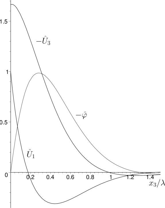
Figure 1: Depth profiles of the mechanical displacements (Å) and the electric potential (V) for the piezoelectric Rayleigh wave in KNbO₃, $Z$-cut $X$-propagation with metallized boundary conditions.

where $\hat{U}_{1}:=\Re\{U_{1}\}$, $\hat{U}_{3}:=\Im\{U_{3}\}$, $\hat{\varphi}:=\Im\{\phi\}$ are the amplitude functions. Figure 1 shows their variations with the scaled depth $x_{3}/\lambda$, where $\lambda=2\pi/k$ is the wavelength. The vertical scaling is such that $U_{1}(0)=1$Å. The axes of the polarization ellipse are along the $x_{1}$ and $x_{3}$ axes. At the interface, $\hat{U}_{1}(0)>0$, $\hat{U}_{3}(0)<0$, and $|\hat{U}_{3}(0)|>|\hat{U}_{1}(0)|$, so that the major axis of the ellipse is along $x_{3}$ and the minor axis is along $x_{1}$; there, the ellipse is spanned in the retrograde sense with time. The ellipse becomes more and more oblong with depth, and is linearly polarized at a depth of about 0.174$\lambda$. Further down the substrate, it becomes elliptically polarized again, but is now spanned in the direct sense. It is circularly polarized at a depth of about 1.183$\lambda$, and then again linearly polarized at a depth of about 0.987$\lambda$.

3.2 Unmetallized boundary condition

For the unmetallized (free) boundary condition, the free surface is in contact with the vacuum (permeability: $\epsilon_{0}$), and so[1],

$$\mbox{\boldmath$\xi$}(0)=\gamma_{1}\begin{bmatrix}a_{1}\\ b_{1}\\ \dfrac{e_{15}}{\epsilon_{33}}c_{1}\\ c_{55}f_{1}\\ c_{55}g_{1}\\ \epsilon_{0}\dfrac{e_{15}}{\epsilon_{33}}h_{1}\end{bmatrix}+\gamma_{2}\begin{bmatrix}a_{2}\\ b_{2}\\ \dfrac{e_{15}}{\epsilon_{33}}c_{2}\\ c_{55}f_{2}\\ c_{55}g_{2}\\ \epsilon_{0}\dfrac{e_{15}}{\epsilon_{33}}h_{2}\end{bmatrix}+\gamma_{3}\begin{bmatrix}a_{3}\\ b_{3}\\ \dfrac{e_{15}}{\epsilon_{33}}c_{3}\\ c_{55}f_{3}\\ c_{55}g_{3}\\ \epsilon_{0}\dfrac{e_{15}}{\epsilon_{33}}h_{3}\end{bmatrix}=\begin{bmatrix}U_{1}(0)\\ U_{3}(0)\\ \varphi(0)\\ 0\\ 0\\ i\epsilon_{0}\varphi(0))\end{bmatrix}.$$ (25)

Similarly to the previous case, the form of $\mbox{\boldmath$\xi$}(0)$ can be found, whatever the form of the $q_{i}$ is. Namely,

$$\mbox{\boldmath$\xi$}(0)=\varphi(0)[i\alpha_{2},\beta_{1},1,0,0,i\epsilon_{0}]^{T},$$ (26)

where $i\alpha_{2}=U_{1}(0)/\varphi(0)$ is pure imaginary ($\alpha_{2}$ is real) and $\beta_{1}=U_{3}(0)/\varphi(0)$ is real. Substitution into the fundamental equations Eqs. (17) at $n=-2,2$ leads to the trivial identity. At $n=-1,1,3$ it leads to

$$M^{(n)}_{33}+\epsilon_{0}^{2}M^{(n)}_{66}+2\epsilon_{0}M^{(n)}_{16}\alpha_{2}+2M^{(n)}_{23}\beta_{1}+M^{(n)}_{11}\alpha_{2}^{2}+M^{(n)}_{22}\beta_{1}^{2}=0,$$ (27)

which are three equations for two unknowns $\alpha_{2}$ and $\beta_{1}$. Formally, solving two equations and substituting the result into the third equation yields the secular equation. Note however that these equations Eqs. (27) are nonlinear (quadratic) in the unknowns. Their resolution is somewhat lengthy, although possible as is now seen.

First take advantage of the identity $M^{(1)}_{23}\equiv N_{56}=0$ to solve Eqs. (27) at $n=1$ for $\beta_{1}^{2}$:

$$\beta_{1}^{2} =-[M^{(1)}_{33}+\epsilon_{0}^{2}M^{(1)}_{66}+2\epsilon_{0}M^{(1)}_{16}\alpha_{2}+M^{(1)}_{11}\alpha_{2}^{2}]/M^{(1)}_{22}$$

$$=[\mu-n_{44}\epsilon_{0}^{2}+2r_{2}\epsilon_{0}\alpha_{2}+(\eta-X)\alpha_{2}^{2})]/X.$$ (28)

Next, solve Eqs. (27) at $n=-1,3$ for $\beta_{1}$:

$$-2\beta_{1}=[M^{(n)}_{33}+\epsilon_{0}^{2}M^{(n)}_{66}+2\epsilon_{0}M^{(n)}_{16}\alpha_{2}+M^{(n)}_{11}\alpha_{2}^{2}+M^{(n)}_{22}\beta_{1}^{2}]/M^{(n)}_{23},$$ (29)

$n=-1,3$. Now square both sides and substitute the expression for $\beta_{1}^{2}$ just obtained to derive two polynomials of fourth degree in $\alpha_{2}$. Having $\alpha_{2}$ as a common root, these two polynomials have a resultant equal to zero, a condition which is the explicit secular equation for the speed of a two-partial Rayleigh piezoacoustic surface wave propagating in an unmetallized 2mm (or 4mm, or 6mm) crystal.

Of course, the resulting polynomial is rather formidable, here of degree 48 in $X$ according to Maple. Nevertheless, finding numerically the roots of a polynomial is a quasi-instantaneous task for a computer. For instance in the case of KNbO₃, it is found that there are 10 positive real roots in $X$ to the polynomial, out of which 6 yield three attenuation factors with positive imaginary part. Out of these 6, only one satisfies the boundary conditions Eqs. (25)₂, that is

$$\dfrac{1}{(q_{1}-q_{2})(q_{2}-q_{3})(q_{3}-q_{4})}\begin{vmatrix}f_{1}&f_{2}&f_{3}\\ g_{1}&g_{2}&g_{3}\\ h_{1}-ic_{1}&h_{2}-ic_{2}&h_{3}-ic_{3}\end{vmatrix}=0.$$ (30)

Hence, at the speed $V_{\text{u}}$ (say) and attenuation factors listed on the third line of Table I (obtained with a 40 digits precision), the determinant in Eq. (30) was found to be smaller than $5\times 10^{-23}$. Note by comparison of the second line and the third line of Table I that when the free surface is metallized, the wave propagates at a slower speed, and is slightly more localized, than when the surface is unmetallized. Figure 2 shows the variations of the amplitude functions with the scaled depth $x_{3}/\lambda$ in the unmetallized boundary conditons case. The depth curves are similar to those in the metallized case, with the differences that the boundary condition forces the electrical potential to be about 0.596 V at the interface, and that the nature of the polarization ellipse changes at depths which are slightly less than the corresponding depths with metallized boundary conditions.

Finally, recall that it is usual to take the quantity $2(V_{\text{u}}-V_{\text{m}})/V_{\text{u}}$ as a measure of the crystal’s ability to transform an electric signal into an elastic surface wave by means of interdigital electrode transducers although, as proved by Royer and Dieulesaint [16], the demonstration is far from obvious. This quantity is often referred to as the effective piezoacoustic coupling coefficient for surface waves and is expected to be positive. In the present example of KNbO₃, the speeds of the second column in Table I give a value of 0.1037, far greater than the corresponding values[13] for GaAS, Bi₁₂GeO₂₀, ZnO, and CdS, and more than twice that [29] for LiNbO₃. Note that Mozhaev and Weihnacht [17] reported negative values for this quantity corresponding to special cuts and propagation direction in KNbO₃.

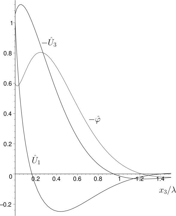
Figure 2: Depth profiles of the mechanical displacements (Å) and the electric potential (V) for the piezoelectric Rayleigh wave in KNbO₃, $Z$-cut $X$-propagation with unmetallized boundary conditions.

References

- [1] B. Collet and M. Destrade, “Explicit secular equations for piezoacoustic surface waves: Shear-Horizontal modes.”, J. Acoust. Soc. Am. 116, 3432–3442 (2004).
- [2] J. L. Bleustein, “A new surface wave in piezoelectric materials”, Appl. Phys. Lett. 13, 412–413 (1968).
- [3] Yu. V. Gulyaev, “Electroacoustic surface waves in piezoelectric materials”, JETP Lett. 9, 37–38 (1969).
- [4] C. -C. Tseng, “Piezoelectric surface waves in cubic crystals”, J. Appl. Phys. 41, 2270–2276 (1970).
- [5] G. G. Koerber and R. F. Vogel, “SH-mode piezoelectric surface waves on rotated cuts”, IEEE Trans. Sonics Ultrason. su-20, 10–12 (1973).
- [6] L. S. Braginskiĭ and I. A. Gilinskiĭ, “Generalized shear surface waves in piezoelectric crystals”, Sov. Phys. Solid State 21, 2035–2037 (1979).
- [7] V. M. Bright and W. D. Hunt, “Bleustein-Gulyaev waves in Gallium Arsenide and other piezoelectric cubic crystals”, J. Appl. Phys. 66, 1556–1564 (1989).
- [8] V. G. Mozhaev and M. Weihnacht, “Sectors of nonexistence of surface acoustic waves in potassium niobate”, IEEE Ultrasonics Symp. Proc. 1, 391–395 (2002).
- [9] I. A. Viktorov, Rayleigh and Lamb waves: physical theory and applications. (Plenum Press, 1967).
- [10] B. Drafts, “Acoustic wave technology sensors”, IEEE Trans. Microw. Theory Tech. 49, 795–802 (2001).
- [11] W. D. Bowers, R. L. Chuan, and T.M. Duong, “A 200 MHz surface acoustic wave resonator mass microbalance”, Rev. Sci. Instrum. 62, 1624–1629 (1991).
- [12] C. Maerfeld and C. Lardat, “Ondes de Love et de Rayleigh dans les milieux piézoélectriques stratifiés (Love and Rayleigh waves in layered piezoelectric media)”, C. R. Acad. Sc. B270, 1187–1190 (1970).
- [13] J. J. Campbell and W. R. Jones, “Propagation of piezoelectric surface waves on cubic and hexagonal crystals”, J. Appl. Phys. 41, 2796–2801 (1970).
- [14] M. Moriamez, E. Bridoux, J. -M. Desrumaux, J. -M. Rouvaen, and M. Delannoy, “Propagation des ondes acoustiques superficielles dans les crystaux piézoélectriques (Propagation of acoustic surface waves in piezoelectric crystals)”, Rev. Phys. Appl. 6, 333–339 (1971).
- [15] E. Bridoux, J. M. Rouvaen, C. Coussot, and E. Dieulesaint, “Rayleigh-Wave Propagation on Bi12GeO20”, Appl. Phys. Lett. 19, 523–524 (1971).
- [16] D. Royer and E. Dieulesaint, Elastic Waves in Solids I: Free and Guided Propagation. (Springer-Verlag, New York, 2000).
- [17] V. G. Mozhaev and M. Weihnacht, “Incredible negative values of effective electromechanical coupling coefficient for surface acoustic waves in piezoelectrics”, Ultrasonics 37 687–691 (2000).
- [18] M. Abbudi and D. M. Barnett, “On the existence of interfacial (Stoneley) waves in bonded piezoelectric half-spaces”, Proc. Roy. Soc. London A 429, 587–611 (1990).
- [19] G. A. Coquin and H. F. Tiersten, “Analysis of excitation and detection of piezoelectric surface waves in quartz by means of surface electrodes”, J. Acoust. Soc. Am. 41, 921–939 (1967).
- [20] The Institute of Electrical and Electronics Engineers, “IEEE Standard on Piezoelectricity”, ANSI/IEEE Std 176-1987.
- [21] J. Lothe and D. M. Barnett, “Integral formalism for surface waves in piezoelectric crystals. Existence considerations”, J. Appl. Phys. 47, 1799–1807 (1976).
- [22] M. Destrade, “Elastic interface acoustic waves in twinned crystals”, Int. J. Solids Struct. 40, 7375–7383 (2003) .
- [23] M. Destrade, “Explicit secular equation for Scholte waves over a monoclinic crystal”, J. Sound Vibr. 273, 409–414 (2004).
- [24] M. Destrade, “On interface waves in misoriented pre-stressed incompressible elastic solids”, IMA J. Appl. Math. 70, 3–14 (2005).
- [25] P. K. Currie, “The secular equation for Rayleigh waves on elastic crystals”, Quart. J. Mech. Appl. Math. 32, 163–173 (1979).
- [26] R. M. Taziev, “Dispersion relation for acoustic waves in an anisotropic elastic half-space”, Sov. Phys. Acoust. 35, 535–538 (1989).
- [27] T.C.T. Ting, “The polarization vector and secular equation for surface waves in an anisotropic elastic half-space”, Int. J. Solids Struct. 41, 2065–2083 (2004).
- [28] M. Zgonik, R. Schlesser, I. Biaggio, E. Voit, J. Tscherry, ans P. Gunter, “Materials constants of KNbO3 relevant for electro- and acousto-optics”, J. Appl. Phys. 74, 1287–1297 (1993).
- [29] G.W. Farnell, “Types and properties of surface waves”, in: A.A. Oliner (ed.) Acoustic Surface Waves, Topics in Applied Physics 24, pp. 13–60 (Springer, Berlin, 1978).
Table I. Wave speed (m s-1) and attenuation coefficients for a two-partial piezoacoustic surface wave in KNbO3.