In-plane electric field effect on a spin-orbit coupled two-dimensional electron system in presence of magnetic field

Abstract

The effect of in-plane electric field on Landau level spacing, spin splitting energy, average spin polarization and average spin current in the bulk as well as at the edges of a two-dimensional electron system with Rashba spin-orbit coupling are presented here. The spin splitting energy for a particular magnetic field is found to be reduced by the external in-plane electric field. Unlike the case of a two-dimensional electron system without Rashba spin-orbit interaction, here the Landau level spacing is electric field dependent. This dependency becomes stronger at the edges in comparison to the bulk. The average spin polarization vector rotates anti-clockwise with the increase of electric field. The average spin current also gets influenced significantly by the application of the in-plane electric field.

I Introduction

The proposal of the possible application of the spin degree of freedom in electronic devices has emerged as a new field called spintronics das1 ; appl1 ; appl2 ; appl3 . The experimental realization of the spin-orbit interaction which lifts the spin degeneracy even in absence of magnetic field has boosted research interest in this field. The Rashba spin-orbit interaction (RSOI) is the particular interest of this field as it’s strength can be enhanced significantly by applying a suitable gate voltage tech ; matsu . The origin of the RSOI is due to the lack of structural inversion symmetry in the semiconductor heterostructures rashba ; rashba1 . The RSOI provides a proficient way to control the electron’s spin degree of freedom. The electric field perpendicular to a two-dimensional electron system (2DES) can enhance the Rashba spin-orbit coupling tech . The RSOI has manifested itself through some remarkable new features in different transport properties dutta ; prl99 ; prl06 ; wang ; wang1 ; firoz . Moreover, spin Hall effect (SHE) is one of the most important consequences of the RSOI in a two-dimensional electron system (2DES). In SHE, electrons with opposite spin polarizations get scattered in transverse direction of the applied electric field even in absence of magnetic field. There have been several theoretical prl99 ; prl06 ; raimondi as well as experimental kato ; sinova works on SHE. The successful detection of spin accumulation kato ; sinova at the edges has made the study of spin current interesting.

The effect of an uniform in-plane electric field on the Landau levels in a two-dimensional system has been always an interesting quantum mechanical problem. The 2DES formed at the semiconductor heterostructure junction, which is also called conventional 2DES and graphene monolayer are two important examples of two-dimensional systems. The spacing between two consecutive Landau levels of a conventional 2DES is independent of electric field. On the other hand, the Landau level spacing in a graphene monolayer depends on the transverse electric field and it can be collapsed under suitable strength of the electric field lukose ; lukose1 ; ngu . These two results are obtained by exact analytical calculation. The Landau levels of the Rashba spin-orbit coupled 2DES show two different energy branches with unequal level spacing wang . The analytical derivation of Landau levels under in-plane electric field seems to be impossible. Therefore, we solve this problem by exact numerical calculation.

The quantum Hall effect has been remained an attractive topic for physicists. The edge states and edge charge currents play very important role in exploring details about quantum Hall effect halperin ; macdonald ; henrik . The spatially well separated left- and right-moving edge states give rise to non-dissipative transport muller ; chang . In presence of the spin-orbit interaction, the transport of the spin-polarized edge channels may provide rich physics. Several theoretical analysis of the spin edge states in a Rashba system has been also reported badalyan ; rose . The crucial role played by the edge states in magnetization zhang and spin polarization bao in 2DES with RSOI has been studied extensively.

In this work, we present the effect of in-plane electric field on Landau level spacing (LLS), spin splitting energy, average spin polarization and average spin current in the bulk as well as at the edges numerically. We find the Landau level spacing and the spin splitting energy decreases with increase of the electric field. The average spin polarization rotates anti-clockwise as we increase electric field. The average spin current is modified due to the presence of the in-plane electric field.

This paper is organized as follows. In Sec. II, we formulate the numerical method to solve the Hamiltonian of a single electron confined in a finite size 2DES with RSOI in presence of crossed electric and magnetic fields. We also discuss the spin-split Landau levels, Landau level spacing, average spin polarization and average spin current of an infinite 2DES with RSOI in presence of magnetic field. In Section III, we present numerical results and discussion of the effect of the transverse electric field on the spin splitting energy, LLS, average spin polarization and average spin current. However, as the energy becomes different at the edges in comparison to the bulk for a finite system, the study of above mentioned properties will also be covered at the edge with electric field. We present summary of our work in Section IV.

II Formalism for Numerical calculation

We consider a spin-orbit coupled 2DES in a $xy$ plane of area $L_{x}\times L_{y}$ which is subjected to an in-plane electric filed $\vec{E}=E\hat{i}$ and magnetic field $\vec{B}=B\hat{z}$. The single-electron Hamiltonian with electronic charge $q=-e$ is given by

$$H = \Big{[}\frac{({\bf p}+e{\bf A})^{2}}{2m^{*}}+V(x)+eEx\Big{]}\sigma_{0}$$ (1)

$$+ \frac{\alpha}{\hbar}[\sigma_{x}(p_{y}+eA_{y})-\sigma_{y}p_{x}]+\frac{g}{2}\mu_{B}B\sigma_{z},$$

where $m^{*}$ is the effective mass of an electron, $\sigma_{0}$ is the $2\times 2$ identity matrix, $\sigma_{i}$ ($i=x,y,z$) are the Pauli matrices, $\alpha$ is the Rashba spin-orbit coupling constant and $V(x)=0$ for $|x|\leq L_{x}/2$ and otherwise infinity is the hard-wall confining potential along the $x$ direction. Also, $g$ is the effective Lande $g$-factor and $\mu_{B}=e\hbar/(2m_{e})$ is the Bohr magneton with $m_{e}$ is the free electron mass. Here, we have chosen the Landau gauge $\vec{A}=Bx\hat{j}$.

Before presenting numerical results, we shall review the bulk Landau levels of a 2DES with RSOI in absence of the electric field. The energy spectrum in the bulk can be obtained analytically by diagonalizing the Hamiltonian wang . The RSOI mixes the two spin components. For $s=0$, there is only one level, same as the lowest Landau level without SOI, with energy $E_{0}^{+}=E_{0}=(\hbar\omega_{c}-g\mu_{B}B)/2$ with $\omega_{c}=eB/m^{*}$. The corresponding wave function is

$$\Psi_{0,k_{y}}^{+}({\bf r})=\frac{e^{ik_{y}y}}{\sqrt{L_{y}}}\phi_{0}(x+x_{0})\left(\begin{array}[]{c}0\\ 1\end{array}\right),$$ (2)

where $x_{0}=k_{y}l_{0}^{2}$ with magnetic length scale $l_{0}=\sqrt{\hbar/(eB)}$. For a given quantum number $s\geq 1$ there are two spin-split branches of energy levels, denoted by $+$ and $-$ with energies

$$E_{s}^{\pm}=s\hbar\omega_{c}{\pm}\sqrt{E_{0}^{2}+sE_{\alpha}\hbar\omega_{c}},$$ (3)

where $E_{\alpha}=2m^{\ast}\alpha^{2}/\hbar^{2}$. The corresponding wave function for $+$ branch is

$$\Psi_{s,k_{y}}^{+}({\bf r})=\frac{e^{ik_{y}y}}{\sqrt{L_{y}A_{s}}}\left(\begin{array}[]{r}D_{s}\phi_{s-1}(x+x_{0})\\ \phi_{s}(x+x_{0})\end{array}\right)\text{,}$$ (4)

and for $-$ branch is

$$\Psi_{s,k_{y}}^{-}({\bf r})=\frac{e^{ik_{y}y}}{\sqrt{L_{y}A_{s}}}\left(\begin{array}[]{r}\phi_{s-1}(x+x_{0})\\ -D_{s}\phi_{s}(x+x_{0})\end{array}\right)\text{,}$$ (5)

where $A_{s}=1+D_{s}^{2}$ with $D_{s}=\sqrt{sE_{\alpha}\hbar\omega_{c}}/[E_{0}+\sqrt{E_{0}^{2}+sE_{\alpha}\hbar\omega_{c}}]$ and $\phi_{s}(x)=(1/\sqrt{\sqrt{\pi}2^{s}s!l_{0}})e^{-x^{2}/2l_{0}^{2}}H_{s}(x/l_{0})$ is the normalized harmonic oscillator wave function. Here, $s$ is the Landau level index.

When both the hard-wall confining potential and the electric field are included, the Hamiltonian given by Eq. (1) has to be solved numerically. To solve the Hamiltonian numerically we choose the following wave function $\Psi(x,y)=(1/\sqrt{L_{y}})e^{ik_{y}y}\phi(x)$ with the function $\phi(x)$ expanded in the basis of the infinite potential well as

$$\phi(x)=\sqrt{\frac{2}{L_{x}}}\sum_{n}\sin\Big{\{}\frac{n\pi}{L_{x}}\Big{(}x+\frac{L_{x}}{2}\Big{)}\Big{\}}\begin{bmatrix}a_{n}\\ b_{n}\end{bmatrix}.$$ (6)

Now, using the time-independent Schrödinger equation, we get the following matrix equations for the spinors:

$$\Big{[} \frac{\hbar^{2}\pi^{2}l^{2}}{2m^{*}L_{x}^{2}}+\frac{g}{2}\mu_{B}\sigma_{z}B\Big{]}\begin{bmatrix}a_{l}\\ b_{l}\end{bmatrix}$$ (7)

$$+ \sum_{n}\Big{[}\sigma_{x}F_{ln}+i\sigma_{y}G_{ln}+M_{ln}+K_{ln}\Big{]}\begin{bmatrix}a_{n}\\ b_{n}\end{bmatrix}=0.$$

Here, the matrix elements are given by

$$F_{ln} = \frac{2\alpha L_{x}}{(\pi l_{0})^{2}}\int_{-\pi/2}^{\pi/2}\sin\Big{\{}l\Big{(}\theta+\frac{\pi}{2}\Big{)}\Big{\}}(\theta+\theta_{0})$$ (8)

$$\times \sin\Big{\{}n\Big{(}\theta+\frac{\pi}{2}\Big{)}\Big{\}}d\theta,$$

$$G_{ln}=\frac{2\alpha n}{L_{x}}\int_{-\pi/2}^{\pi/2}\sin\Big{\{}l\Big{(}\theta+\frac{\pi}{2}\Big{)}\Big{\}}\cos\Big{\{}n\Big{(}\theta+\frac{\pi}{2}\Big{)}\Big{\}}d\theta,$$ (9)

$$M_{ln} = \frac{m^{*}\omega_{c}^{2}L_{x}^{2}}{\pi^{3}}\int_{-\pi/2}^{\pi/2}\sin\Big{\{}l\Big{(}\theta+\frac{\pi}{2}\Big{)}\Big{\}}(\theta+\theta_{0})^{2}$$ (10)

$$\times \sin\Big{\{}n\Big{(}\theta+\frac{\pi}{2}\Big{)}\Big{\}}d\theta$$

and

$$K_{ln}=\frac{2eEL_{x}}{\pi^{2}}\int_{-\pi/2}^{\pi/2}\sin\Big{\{}l\Big{(}\theta+\frac{\pi}{2}\Big{)}\Big{\}}\theta\sin\Big{\{}n\Big{(}\theta+\frac{\pi}{2}\Big{)}\Big{\}}d\theta,$$ (11)

where $\theta=\pi x/L_{x}$, $\theta_{0}=\pi x_{0}/L_{x}$.

We solve these equations numerically in a truncated Hilbert space by considering $400\times 400$ matrix Hamiltonian and confirmed that first thirty eigenvalues in the bulk with ${\bf E}=0$ exactly match with the results obtained from the analytical expression. Also, the probability density of the corresponding low-energy states are in excellent agreement with the analytical results. We have numerically checked that in presence of the electric field $E$, the cyclotron center $x_{0}$ in the bulk is displaced by $x_{E}=eE/(m^{*}\omega_{c}^{2})$ from right to left side. For low-lying Landau levels, the electric field induced displacement $x_{E}$ is almost independent of $s$. When $x_{0}\approx 0$ the states are far away from the boundary and called bulk states. When $x_{0}\approx\pm L_{x}/2$ the states are close to the boundary and called edge states.

We define the spin splitting energy for a given Landau level $s$ as $\Delta_{s}=E_{s}^{+}-E_{s}^{-}$. In the bulk with $E=0$, $\Delta_{s}=2\sqrt{E_{0}^{2}+sE_{\alpha}\hbar\omega_{c}}$. It implies that the spin splitting energy $\Delta_{s}$ is increasing with increase of $s$, $\alpha$ and $B$. The LLS between two consecutive Landau levels is defined as $\Delta E_{s}^{\pm}=E_{s+1}^{\pm}-E_{s}^{\pm}$. The total of the LLS for spin-up and spin-down branches is $\Delta E_{s}=\Delta E_{s}^{+}+\Delta E_{s}^{-}=2\hbar\omega_{c}$. This is independent of $\alpha$ and Landau level index $s$.

The components of the average spin polarization are defined as

$$P_{s}^{\lambda,S_{i}}(k_{y})=\frac{\hbar}{2}\int d^{2}r\Big{[}\Psi_{s,k_{y}}^{\lambda}({\bf r})\Big{]}^{\dagger}\sigma_{i}\Psi_{s,k_{y}}^{\lambda}({\bf r}),$$ (12)

where $i=x,y,z$ and $\lambda=\pm$ represents the spin-up and spin-down components. The $y$ component of the average spin polarization is always zero. In absence of the electric field, the average spin polarization components can be evaluated analytically. In the bulk, the average spin polarization of the ground state ($s=0$) is along the +$z$ axis. In the excited states ($s\geq 1$), the average spin polarization in the bulk is $P_{s}^{\lambda,S_{z}}=\lambda(\hbar/2)(1-|D_{s}|^{2})/A_{s}$. For a given $s$, the spin polarization of $+$ branch is anti-parallel to that of the $-$ branch.

The spin current density for a given Landau level $s$ is given by $J_{s,y}^{\lambda,S_{i}}({\bf r})=[\Psi_{s,y}^{\lambda}]^{\dagger}\hat{J}_{y}^{S_{i}}\Psi_{s,y}^{\lambda}$, where $\hat{J}_{y}^{S_{i}}$ are the spin current operators with $i=x,y,z$. We use the conventional definition of the spin current operator as $\hat{J}_{y}^{S_{x}}=\hbar\hat{v}_{y}\sigma_{x}/2$ and $\hat{J}_{y}^{S_{z}}=\hbar(\hat{v}_{y}\sigma_{z}+\sigma_{z}\hat{v}_{y})/4$. The $y$ component of the velocity operator is given by $\hat{v}_{y}=(x+x_{0})\omega_{c}\sigma_{0}+\frac{\alpha}{\hbar}\sigma_{x}$. The average spin current is defined as $\langle J_{s,y}^{S_{i}}\rangle=\sum_{\lambda}J_{s,y}^{\lambda,S_{i}}=\sum_{\lambda}\int d^{2}rJ_{s,y}^{\lambda,S_{i}}({\bf r})$. In absence of the electric field, the average $x$-component spin current carried by a given Landau level can be easily obtained and it is given by $\langle J_{s,y}^{S_{x}}\rangle=\alpha$, independent of the Landau level index $s$. On the other hand, $z$ component of average spin current is $\langle J_{s,y}^{S_{z}}\rangle=0$. A point to be noted here that average spin current is linearly dependent on $\alpha$ and independent of magnetic field strength. On the other hand, the total spin current in absence of magnetic field is cubic in $\alpha$ sonin . Following Ref.bao , one can easily show that even in presence of electric field the spin current $J_{s,y}^{\lambda,S_{z}}$ is proportional to $P_{s}^{\lambda,S_{x}}$: $J_{s,y}^{\lambda,S_{z}}=-\frac{g\hbar\mu_{B}B}{2m^{*}}P_{s}^{\lambda,S_{x}}$. This kind of relation does not hold between $J_{s,y}^{\lambda,S_{x}}$ and $P_{s}^{\lambda,S_{z}}$.

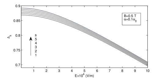
Figure 1: Plots of the spin splitting energy in the bulk versus electric field for few $s$ values.

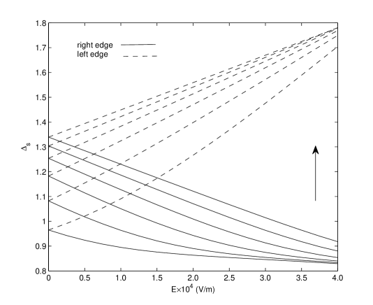
Figure 2: Plots of the spin splitting energy at the edges versus electric field for few $s$ values.

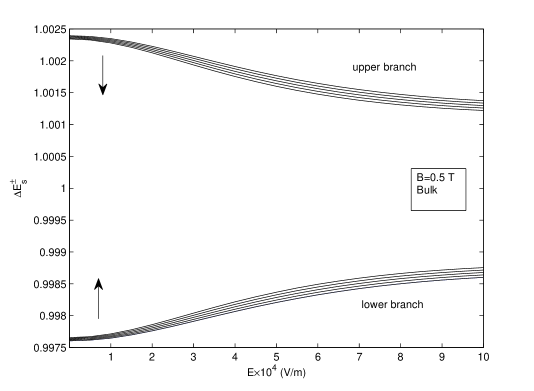
Figure 3: Plots of the Landau level spacing in the bulk versus electric field for few $s$ values.

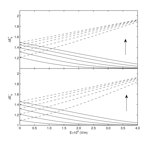
Figure 4: Plots of the Landau level spacing versus electric field for few $s$ values. Here, dashed and solid lines represent left and right edges.

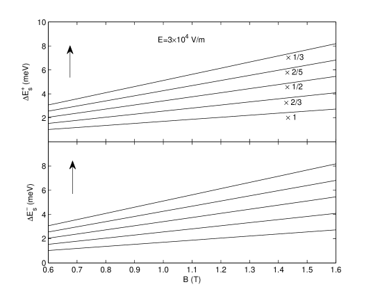
Figure 5: Plots of the Landau level spacing in the bulk versus magnetic field for the fixed electric field. For better visualization, each curve is magnified by a suitable constant number as indicated in the figure.

III Numerical result and analysis

For the numerical calculation, we use the following parameters: system size $L_{x}=L_{y}=1200$ nm, electron’s effective mass $m^{*}=0.068m_{e}$, Rashba spin-orbit coupling constant $\alpha=0.1\alpha_{0}$ with $\alpha_{0}=10^{-11}$ eV-m. Selective numerical parameters have been chosen to satisfy the following conditions: cyclotron radius $R_{c}\sim l_{0}<L_{x}/2$ and the shift of the cyclotron orbit’s center due to the maximum applied electric field $(x_{E})_{\rm max}+x_{0}<L_{x}$. Here, $(x_{E})_{\rm max}=154$ nm for maximum $E=5\times 10^{4}$ V/m and $B=0.5$ T. To describe the left and right edge states, we have taken $k_{y}=\pm 0.44L_{x}/l_{0}^{2}$. Therefore, the left and right edges are far away from each other in real space. We have also taken $k_{y}=0$ to describe the bulk states.

III.1 Spin splitting and Landau level spacing

In the previous section, we have seen that the spin splitting energy and the LLS in the bulk can be controlled by tuning the magnetic field. Here, we will see these quantities can also be controlled by the transverse electric field. The spin splitting energy and LLS are plotted in units of $\hbar\omega_{c}$. In Fig. 1, we show how $\Delta_{s}$ in the bulk varies with $E$. Figure 1 shows that the spin splitting energy is diminishing with the increase of the applied transverse electric field. It implies that electric field effectively reduces the effect of the RSOI in presence of the perpendicular magnetic field. In Fig. 2, we plot $\Delta_{s}$ at the two edges versus electric field. Comparing Fig. 1 and Fig. 2, it is seen that the spin splitting energy at the edges is large compared to that of the bulk region when $E=0$. The spin splitting energy at the left edge is increasing with increase of electric field. On the other hand, $\Delta_{s}$ at the right edge is decreasing with increase of $E$. This is due to the fact that cyclotron orbit shifts from right to left with increasing electric field. The states around the left edge shifts towards the left boundary where as the states around right edge moves towards the bulk region. Thats why the spin splitting energy of the left and right edge states increases and decreases with electric field, respectively. Moreover, the spin-splitting energy at the edges changes almost linearly with $E$ whereas $\Delta_{s}$ in the bulk decreases non-linearly with $E$.

In Fig. 3, we show how LLS for spin-up and spin-down branches in the bulk varies with $E$. The LLS for upper branches decreases where as for lower branches it increases with the electric field. This is in complete contrast to the case of a 2DES without RSOI where LLS does not depend on the transverse electric field. But, it is similar to the LLS in graphene case. Moreover, for strong enough electric field, the LLS for spin-up and spin-down branches tends to saturate to $\hbar\omega_{c}$ which is the same as in the absence of RSOI. The reduction in the spin splitting energy and saturation in LLS in the bulk can be understood from the fact that when electric field is sufficiently high the effective Rashba coupling becomes very weak. It is interesting to note that $\Delta E_{s}=\Delta E_{s}^{+}+\Delta E_{s}^{-}$ is always $2\hbar\omega_{c}$ even in presence of electric field. We also plot LLS at the edges versus electric field in Fig. 4.

In Fig. 5, we show the LLS as a function of magnetic field when the transverse electric field is fixed. It shows that both $\Delta_{s}^{+}$ and $\Delta_{s}^{-}$ increase with magnetic field. The slope of $\Delta_{s}^{+}$ is slightly higher than that of the $\Delta_{s}^{-}$.

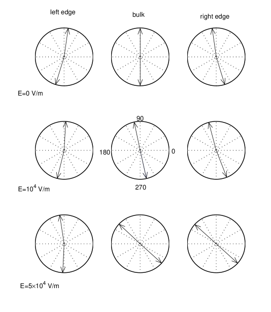
Figure 6: Diagrams of the average spin polarization vectors at various locations for different electric field strength.

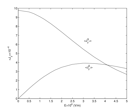
Figure 7: Plots of the average spin current for $x$ and $z$ components versus electric field in the bulk. The average spin current is in units of $\hbar\omega_{c}L_{x}$.

III.2 Average spin polarization

The average spin polarization vector versus electric field at different locations of the center of the cyclotron orbit is shown in Fig. 6. The increasing order of rows are accompanied with the increasing electric field whereas the columns are associated with the three different locations of the cyclotron center i.e. left edge, bulk and right edge. The arrow line in the upper-half and lower-half circle stands for spin-up and spin-down branches, respectively.

The top panel shows the average spin polarization vector in absence of the electric field. In the bulk, the average spin polarization vector is solely along the $\pm z$ direction for spin-up and spin-down branches, respectively. At the edges the spin polarization vector lies in the $xz$ plane. The magnitudes of the components of the spin polarization vector depend on the location of the electron. It is interesting to note that the spin polarization vectors at the left and rights edges for $+$ branch and $-$ branch are not anti-parallel to each other. This is due to strong spin splitting at the edges as seen in Fig. 2.

When a suitable electric field is applied, the average spin polarization vectors for up and down states start to rotate anti-clockwise. The amount of spin rotation is solely determined by the electric field and location. The electric field effect on the spin polarization vector at the left edge is smaller compared to the bulk and right edge. This is because of the $k_{y}$ dependent asymmetric energy spectrum in presence of electric field. The anti-clockwise rotation of the average spin-polarization vector due to the electric field can be observed experimentally by Kerr rotation method.

III.3 Spin current

Figure 7 shows that in the bulk the average $x$ component spin current carried by the Landau level $s=2$ is destroyed rapidly from the maximum value $\alpha$ due to the electric field, whereas the average $z$ component spin current starts to increase from zero. After certain electric field strength, it starts to decrease slowly with the increase of the electric field. We have checked that the upper and lower component of the $z$-component spin current individually follows the relation between spin polarization and spin current i.e; with increasing $x$-component of polarization the $z$-component spin current increases. But the total $z$ component spin current does not follow this after a certain electric field strength as shown in the figure.

In Fig. 8, we show how the average $x$ and $z$ components of the spin current carried by $s=2$ Landau level change as we increase magnetic field for a fixed electric field. The spin polarization along $z$ axis increases with increase of the magnetic field. In other words, the spin polarization along $x$ axis decreases with increase of the magnetic field. The average spin current $J_{s,y}^{\lambda,S_{z}}$ will decrease with magnetic field since $J_{s,y}^{\lambda,S_{z}}=-\frac{g\hbar\mu_{B}B}{2m^{*}}P_{s}^{\lambda,S_{x}}$. Our numerical result is consistent with the exact analytical results.

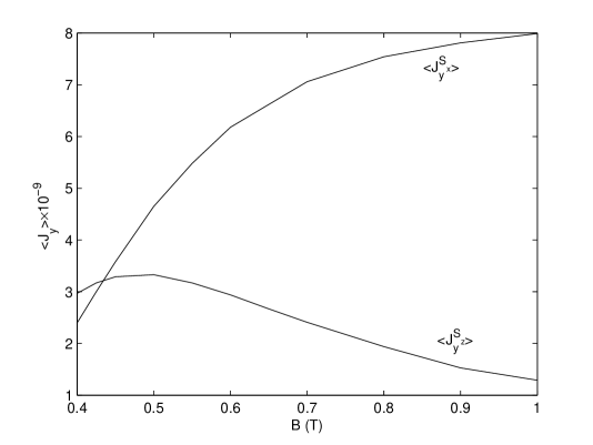
Figure 8: Plots of the average spin current for $x$ and $z$ components versus magnetic field in the bulk. The average spin current is in units of eV-$L_{x}$.

IV Conclusion

We have studied thoroughly the effect of the electric field on the 2DES with Rashba SOI when the system is under a perpendicular magnetic field. The spin splitting energy in the bulk is diminishing with the applied transverse electric field. The Landau level spacing between two successive Landau levels for upper or lower branches gets influenced by electric field. This result is in contrast to the 2DES without RSOI, but it is similar to the graphene case. The LLS for upper or lower branches tends to saturate to $\hbar\omega_{c}$ for strong enough electric field. These results indicate that strong transverse electric field can effectively reduces the effect of the RSOI in presence of magnetic field. The electric field also has a strong influence on the spin polarization vector depending on the different location of electron. The average spin polarization vector rotates anti-clockwise as we increase electric field. The $x$-component of the spin current is destroyed very fast by the applied electric field whereas the $z$-component of spin current increases initially then decays slowly. On the other hand, when electric field is fixed and magnetic field is varying, the $z$-component of the spin current decreases slowly after a certain magnetic field and $x$-component of the spin current increases very fast.

V Acknowledgement

This work was financially supported by the CSIR, Govt. of India under the grant CSIR-SRF-09/092(0687) 2009/EMR F-O746.

References

- (1) S. Datta and B. Das, Appl. Phys. Lett. 56, 665 (1990)
- (2) I. Zutic, J. Fabian, and S. Das Sarma, Rev. Mod. Phys. 76, 323 (2004)
- (3) A. Wolf et al, Science 294, 1488 (2001)
- (4) D. D. Awschalom and M. E. Flatte, Nature Phys 3, 153 (2007)
- (5) J. Nitta, T. Akazaki, H. Takayanagi, and T. Enoki, Phys. Rev. Lett. 78, 1335 (1997)
- (6) T. Matsuyama, R. Kursten, C. Meibner, and U. Merkt, Phys. Rev. B 61, 15588 (2000)
- (7) E. I. Rashba and V. I. Sheka, Fizika Tverdogo Tela; Collected Papers vol 2 (Moscow and Leningrad: Academy of Sciences of the USSR) 162 (1959); E. I. Rashba, Sov. Phys.-Solid State 2, 1109 (1960)
- (8) Y. A. Bychkov and E. I. Rashba, J. Phys. C: Solid State, 17, 6039 (1984)
- (9) B. Das, D. C. Miller, S. Datta, R. Reifenberger, W. P. Hong, P. K. Bhattachariya, J. Sing, and M. Jaffe, Phys. Rev. B 39, 1411 (1989)
- (10) J. E. Hirsch, Phys. Rev. Lett. 83, 1834 (1999)
- (11) B. A. Bernevig and S. C. Zhang, Phys. Rev. Lett. 96 106802 (2006)
- (12) X. F. Wang and P. Vasilopoulos, Phys. Rev. B 67, 085313 (2003)
- (13) X. F. Wang, P. Vasilopoulos, and F. M. Peeters, Phys. Rev. B 71, 125301 (2005)
- (14) SK Firoz Islam and T. K. Ghosh, J. Phys.: Condens. Matter 24, 185303 (2012)
- (15) P. Lucignano, R. Raimondi, and A. Tagliacozzo, Phys. Rev. B 78, 035336 (2008)
- (16) Y. K. Kato, R. C. Myers, A. C. Gossard, and D. D. Awschalom, Science 306, 1910 (2004)
- (17) J. Wunderlich, B. Kaestner, J. Sinova, T. Jungwirth, Phys. Rev. Lett. 94, 047204 (2005)
- (18) V. Lukose, R. Shankar, and G. Baskaran, Phys. Rev. Lett. 98, 116802 (2007)
- (19) N. M. R. Peres and E. V. Castro, J. Phys.: Condens. Matter 19, 406231 (2007)
- (20) N. Gu, M. Rudner, A. Young, P. Kim, and L. Levitov, Phys. Rev. Lett. 106, 066601 (2011)
- (21) B. I. Halperin, Phys. Rev. B 25, 2185 (1982)
- (22) A. H. Macdonald and P. Streda, Phys. Rev. B 29, 1616 (1984)
- (23) A. Strom, H. Johannesson, and G. I. Japaridze, Phys. Rev. Lett. 104, 256804 (2010)
- (24) G. Muller, D. Weiss, A. V. Khaetskii, K. von Klitzing, S. Koch, H. Nickel, W. Schlapp, and R. Losch, Phys. Rev. B 45, 3932 (1992)
- (25) A. M. Chang, Rev. of Mod. Phys. 75, 1449 (2003)
- (26) V. L. Grigoryan, A. M. Abiague, and S. M. Badalyan, Phys. Rev. B 80, 165320 (2009)
- (27) A. Reynoso, G. Usag, M. J. Sanchez, and C. A. Balseiro, Phys. Rev. B 70, 235344 (2004)
- (28) Z. Wang, W. Zhang, and P. Zhang, Phys. Rev. B 79, 235327 (2009)
- (29) Y. Bao, H. Zhuang, S. Shen, and F. Zhang, Phys. Rev. B 72, 245323 (2005)
- (30) E. B. Sonin, Phys. Rev. B 76, 033306 (2007)