Pulse phase dependent variations of the cyclotron absorption features of the accreting pulsars A 0535+26, XTE J1946+274 and 4U 1907+09 with Suzaku

Abstract

We have performed a detailed pulse phase resolved spectral analysis of the cyclotron resonant scattering features (CRSF) of the two Be/X-ray pulsars A0535+26 and XTE J1946+274 and the wind accreting HMXB pulsar 4U 1907+09 using Suzaku observations. The CRSF parameters vary strongly over the pulse phase and can be used to map the magnetic field and a possible deviation form the dipole geometry in these sources. It also reflects the conditions at the accretion column and the local environment over the changing viewing angles. The pattern of variation with pulse phase are obtained with more than one continuum spectral models for each source, all of which give consistent results. Care is also taken to perform the analysis over a stretch of data having constant spectral characteristics and luminosity to ensure that the results reflect the variations due to the changing viewing angle alone. For A0535+26 and XTE J1946+274 which show energy dependent dips in their pulse profiles, a partial covering absorber is added in the continuum spectral models to take into account an additional absorption at those phases by the accretion stream/column blocking our line of sight.

1 Introduction

The X-ray binary sources in which the compact object is a highly magnetized neutron star, often with a massive companion are called accretion powered pulsars. Due to the strong magnetic field of the neutron star, the matter here flows along the magnetic field lines to the poles of the system, forming an X-ray emitting accretion column above it (Pringle & Rees, 1972; Davidson & Ostriker, 1973; Lamb et al., 1973). Another important consequence of the strong magnetic fields ($\sim 10^{12}$ G) are the cyclotron resonant scattering features (CRSFs) formed by the resonant scattering of photons by the electrons which are quantized into Landau levels forming absorption like features at multiples of $E_{c}=11.6keV\times\frac{1}{1+z}\times\frac{B}{10^{12}G}$, $E_{c}$ being the centroid energy, z the gravitational redshift and B the magnetic field strength of the neutron star. The CRSFs thus provide a direct tool to measure the magnetic field strength of the neutron star. It was first discovered in the spectrum of Her X-1 (Trümper et al., 1977; Truemper et al., 1978) and about 20 sources with CRSFs have been discovered so far (Pottschmidt et al., 2012). The CRSFs which are found mostly in high mass X-ray binaries, about a half of which are transient sources, lie between the energy range of 10-60 keV. In addition to the magnetic field strength, the CRSFs also provide crucial information on the emission geometry and its physical parameters like the electron temperature, optical depth etc.
Pulse phase resolved spectroscopy of the cyclotron parameters is an especially useful tool to probe the emission geometry at different viewing angle as the neutron star rotates. It can further be used to map the magnetic field geometry of the neutron star. Since the CRSFs also show variations with luminosity and spectral changes, to perform pulse phase resolved analysis, care should be taken to obtain the results solely due to the changing viewing angle by averaging over the data stretch with similar counts and spectral ratios. Proper continuum modeling of the energy spectrum also plays an important role in phase resolved analysis. Suzaku, with its broadband energy coverage is most ideally suited in this regard.

A0535+26 is a Be/X-ray binary pulsar which was discovered during a giant outburst in 1975 by Ariel V (Rosenberg et al., 1975). It consists of a 103 s pulsating neutron star with a O9.7IIIe optical companion HDE245770 (Bartolini et al., 1978) in an eccentric orbit of e=0.47, with orbital period of 111 days (Finger et al., 2006). The distance to the source is $\sim$ 2 kpc (Giangrande et al., 1980; Steele et al., 1998). Upto six giant outbursts have been detected in this source so far, the latest ones during 2009/2010 (Caballero et al., 2011a, b). The last giant outburst was followed by two smaller outbursts with a periodicity of 115 days which is longer than its orbital period. Precursors to the giant outburst was also observed with the same periodicity (Mihara et al., 2010). CRSFs at $\sim$ 45 keV and $\sim$ 100 keV were discovered in this source during the 1989 giant outburst with HEXE (Kendziorra et al., 1994). The second harmonic at $\sim$ 110 keV was confirmed with OSSE during the 1994 outburst (Grove et al., 1995), although the presence of the fundamental at $\sim$ 45 keV was dubious. It was later confirmed during the 2005 outburst with Integral, RXTE (Caballero et al., 2007) and Suzaku observations (Terada et al., 2006).

XTE J1946+274 is a transient Be/X-ray binary pulsar discovered by ASM onboard RXTE (Smith et al., 1998), and CGRO onboard BATSE (Wilson et al., 1998) during a giant outburst in 1998, revealing 15.8 s pulsations. The optical counterpart was identified as an optically faint B $\sim$ 18.6 mag, bright infrared (H $\sim$ 12.1) Be star (Verrecchia et al., 2002). The source has a moderately eccentric orbit of 0.33 with an orbital period of 169.2 days (Paul et al., 2001; Wilson et al., 2003). After the initial giant outburst and several short outbursts at periodic intervals, the source went into quiescence for a long time until the recent outburst in 2010 (Caballero et al., 2010b). A CRSF was discovered at $\sim$ 35 keV from the RXTE data of the 1998 outburst observations (Heindl et al., 2001).

4U 1907+09 is a persistent wind accreting high mass X-ray binary discovered in the Uhuru surveys (Giacconi et al., 1971; Schwartz et al., 1972), having a highly redenned companion star (O8-O9 Ia) of magnitude 16.37 mag and a mass loss rate of $\dot{M}=7*10^{-6}M\odot yr^{-1}$ (Cox et al., 2005). It has a moderately eccentric (e=0.28) orbit of 8.3753 days (in ’t Zand et al., 1998). It is a slowly rotating neutron star with period of $\sim$ 440 s, and has showed several episodes of torque reversals with a steady spin-down from 1983 to 1998 (in ’t Zand et al., 1998; Mukerjee et al., 2001), a much slower spin-down from 1998 to 2003 (Baykal et al., 2006), a torque reversal between 2004 and 2005 (Fritz et al., 2006) and a second torque reversal between 2007 and 2008 (Inam et al., 2009), which restored the source to the same spin-down rate before 1998. A CRSF at $\sim$ 19 keV was reported using data from the Ginga /observations (Makishima & Mihara, 1992; Makishima et al., 1999) and was later confirmed from the BeppoSaX observations with the discovery of a harmonic at $\sim$ 36 keV. (Cusumano et al., 1998). Rivers et al. (2010) performed a time and phase resolved analysis of the Suzaku observations of the source made during 2006 and 2007.
Here we present the results obtained from a pulse phase resolved spectroscopic analysis of these three sources with a motivation to investigate the variation pattern of the cyclotron parameters with pulse phase. The pulse phase dependence of the CRSF parameters are presented for the first time for A0535+26 and XTE J1946+274, whereas a more detailed result is presented for 4U 1907+09 which is in agreement with the earlier results of Rivers et al. (2010). The analysis is done taking into account various factors which might smear the pulse phase dependence results.The results presented in this paper are one of the most detailed results on pulse phase resolved measurements of CRSF available so far.

2 Observations & Data Reduction

There are two sets of scientific instruments onboard Suzaku. The X-ray Imaging Spectrometer XIS (Koyama et al., 2007) consisting of three front illuminated CCD detectors (FI :XIS0, XIS2, XIS3) and one back illuminated CCD detector (BI: XIS1) work in the 0.2-12 keV range and the Hard X-ray Detector (HXD) made of PIN diodes (Takahashi et al., 2007) and GSO crystal scintillator detectors cover the energy bands of 10-70 keV and 70-600 keV respectively.

Suzaku (Mitsuda et al., 2007) observed A0535+26 twice, once on September 14–15 2005 during the decline of the second normal outburst of 2005, and again on August 24 2009 during the decline of the 2009 normal outburst. We have chosen the 2009 observation (Obs. Id–404054010) for our analysis because of the longer duration (exposure $\sim$ 52 ks) and its ’HXD nominal’ pointing position which is more suitable for CRSF studies, although the count rates were comparable for both the observations. The XIS’s were operated in the ’$\frac{1}{4}$ window’ ’burst’ clock data mode which has a total time resolution of 2 s.
 XTE J1946+274 was observed on October 11 2010 (Obs. Id–405041010) just after the peak of the September/October 2010 normal outburst. The source was observed for $\sim$ 51 ks in the ’HXD nominal’ pointing position, and the XIS’s were operated in the ’$\frac{1}{4}$ window’ ’normal’ clock data mode which has a time resolution of 2 s.
4U 1907+09 was also observed twice with Suzaku, once on May 2006, and again on April 2007. We have chosen the 2007 observation (Obs. Id–402067010) for our analysis because of similar reasons as in the case of A0535+26, i.e. longer exposure of $\sim$ 158 ks and the ’HXD nominal’ pointing position. The XIS’s were operated in ’normal’ clock data mode with no window option which has a time resolution of 8 s. The XIS data was reduced and extracted from the unfiltered XIS events, which were reprocessed with the CALDB version 20120428. We checked for any significant photon pile-up effect in the reprocessed XIS event files. To perform pile-up estimation, we examined the Point Spread Function (PSF) of the XIS’s and obtained the count rate at the image peak per CCD exposure as given by Yamada & Takahashi (Yamada et al., 2012). Crab data is assumed to be free from pile-up and has a value of 36 $ct/sq\,arcmin/s/CCD\,exposure$ at the image peak. Following their procedure, the XIS data of A0535 +26 and XTE J1946+274 had values of 2-3 $ct/sq\,arcmin/s/CCD\,exposure$ at the image peaks, and showed no evidence of significant pile-up. 4U 1907+09 on the other hand showed a case of moderate photon pile-up. The value obtained at the image center was higher than the Crab Nebula count rate of 36 $ct/sq\,arcmin/s/CCD\,exposure$. The radius at which this value equals 36 in the PSF is about 15-16 arcsec, and hence 15 pixels were removed from the image center to account for this effect. For the extraction of XIS light curves and spectra from the reprocessed XIS data, a $4^{{}^{\prime}}$ diameter circular region was selected around the source centroid for A0535+26 and XTE J1946 +274, and an additional central 15 ($\sim$ $16^{{}^{\prime\prime}}$) pixels were removed in the case of 4U 1907+09 to discard the maximum pile up affected regions. Background light curves and spectra were also extracted by selecting regions of the same size away from the source. The XIS count rate was 3.6 c/s, 3.1 c/s and 8.1 c/s for A0535+26, XTE J1946 +274 and 4U 1907+09 respectively. 4U 1907+09 had a $\sim 12$ % loss in count rate after the removal of the photons from the central region due to the pile-up correction. Response files and effective area files were generated by using the FTOOLS task ’xisresp’. The HXD/PIN light curves and spectra were extracted after reprocessing the unfiltered event files . The HXD/PIN background was created by adding the simulated ’tuned’ non X-ray background event files (NXB) corresponding to the month and year of the respective observations Fukazawa et al. (2009) to the the cosmic X-ray background, which was simulated as suggested by the instrument team after applying appropriate normalizations for both cases. The corresponding response files were obtained from the Suzaku guest observatory facility.

3 A 0535+26 and XTE J1946+274

3.1 Timing analysis: Light curves & Hardness ratio & pulse period determination

We performed timing analysis after applying barycentric corrections to the event data files using the FTOOLS task ’aebarycen’. Light curves were extracted with a time resolution of 2 s for the XISs (0.2–12 keV), and 1 s for the HXD/PIN (10–70 keV) respectively. For XTE J1946+274 which has a short pulse period, light curve with the resolution of 10 ms was extracted from the HXD/PIN data to search for the pulse period. We applied pulse folding and $\chi^{2}$ maximization technique to search for pulsations in the XIS data for A 0535+26 and PIN/HXD data for XTE J1946+274. The best estimate of the period was found to be $103.47\pm 0.09$ s for A0535+26. This value is consistent with the pulse period determined from the INTEGRAL IBIS data during the same outburst at MJD 55054.995 (Caballero et al., 2010a) assuming the spin down value determined from the same. For XTE J1946+274, the best-fit period was estimated to be $15.75\pm 0.11$ s. Orbital correction of the pulse arrival times was not required for both the sources having a very long orbital period. The XIS and PIN light curves of the sources binned with its pulse period for A 0535+26 and 10 pulsar periods for XTE J1946+274, are shown in Figure 1. The light curves show more or less constant count rate, and do not have any particular trend of variation. For each figure, the third panel shows the hardness ratios (ratio of PIN counts to XIS counts) which is also more or less constant throughout the observation duration and does not have any signatures of spectral variability which might affect the results of pulse phase resolved spectroscopy.

3.2 Energy Dependence of the pulse profiles

We created the energy resolved pulse profiles for the entire stretch of observations by folding the light curves in different energy bands with the obtained pulse period. The pulse profiles in the energy range of 0.3-12 keV were created using all the three XISs (0, 1 & 3), and in the 10-70 keV range were created from the PIN data. The energy dependence of the pulse profiles in A 0535+26 are shown in Figure 2. The pulse profiles are complex in structure with narrow dips in the low energy ranges $\leq 12$ keV which morphed to become a simpler, more sinusoidal profile at higher energies. The following characteristics are observed with a careful examination of the profiles.

1. A narrow dip at phase $\sim$ 0.1, which decreases in strength with energy and disappears at energies $\geq 14$ keV.

2. Indication of another sharp dip at phases $\sim$ 0.2–0.3, which is evident only at the lowest energy range ($\leq 2$keV).

3. The emission component between phases 0.5–0.7 becomes weaker and weaker with energy and finally disappears at $\sim$ 17 keV. As a result the main dip of the profile (at phase $\sim 0.6$) is narrower at lower energies ($\leq 12$ keV) and broader at higher energies

The energy dependence is very similar to that found during the 2005 Suzaku observation (Naik et al., 2008). The profile is however, very different from the simple sinusoidal profile at all energies found during the quiescence phase of the source (Mukherjee & Paul, 2005; Negueruela et al., 2000), or the double peaked profile extending upto higher energies during its giant outbursts (Mihara, 1995; Kretschmar et al., 1996).

The energy dependence of the pulse profiles of XTE J1946+274 is shown in Figure 3. The pulse profiles show a clear double peaked structure which extends upto the high energies. The following characteristics can be observed in more detail.

1. At the lowest energy ranges (0.3–4 keV), the peak (phase $\sim$ 0.5) increases in strength with energy and the dip at phase $\sim$ 0.8 increases in strength.

2. Between 4–7 keV, the same dip mentioned above decreases in strength and the two peaks are almost equal in strength.

3. Between 7–17 keV, this dip (phase $\sim$ 0.8) disappears and a new, much weaker dip appears at $\sim$ 0.9 which is probably the true interpulse region between the pulses.

4. At the highest energies (25–70 keV), the second peak at phase $\sim$ 0.1 becomes much weaker.

The energy dependence of the pulse profiles of XTE J1946+274 is very similar to that investigated by Wilson et al. (2003) during the 1998 outburst of the source.

3.3 Spectroscopy

3.3.1 Pulse phase averaged spectroscopy

We performed pulse phase averaged spectral analysis of A 0535+26 and XTE J1946+274 using spectra from the three front illuminated CCDs (XISs-0 and 3), the back illuminated CCD (XIS-1) and the PIN. We performed spectral fitting using XSPEC v12.7.0. The XIS spectra were fitted from 0.8-10 keV and the PIN spectrum from 10-70 keV. The energy range of 1.75-2.23 keV was neglected due to an artificial structure in the XIS spectra around the Si edge and Au edge. After appropriate background subtraction, the spectra were fitted simultaneously with all parameters tied, except the relative instrument normalizations which were kept free. The XIS spectra were rebinned by a factor of 6 from 0.8-6 keV and 7-10 keV, and by a factor of 2 between 6-7 keV. The PIN spectrum of A 0535+26 was rebinned by a factor of 2 upto 22 keV, by 4 upto 45 keV, and 6 upto 70 keV. Due to comparatively inferior statistics in the PIN spectrum of XTE J1946+274, higher rebinning factors of 2, 6, and 10 were applied in the above mentioned energy ranges.
In HMXB accretion powered pulsars, the continuum emission can be interpreted to arise by Comptonization of soft X-rays in the plasma above the neutron star surface. It is usually modeled phenomenologically with a powerlaw and cutoff at high energies (White et al., 1983; Mihara, 1995; Coburn, 2001). The most widely used empirical models are the high energy cutoff (highecut) or the Fermi Dirac cutoff (fdcut) (Tanaka, 1986) with the powerlaw component, or cutoff powerlaw (cutoffpl) model. Other models include the negative-positive exponential powerlaw component (NPEX) (Mihara, 1995), and a more physical comptonization model ’CompTT’ (Titarchuk, 1994). We tried to fit the energy spectra with all the continuum models mentioned above, available as a standard or local package in XSPEC and carried out further analysis with only the models which gave best fits for the respective sources.

A 0535+26 :

For A0535+26 the best fits were obtained with the NPEX, powerlaw and the ’CompTT’ model (assuming spherical geometry for the comptonizing region). The powerlaw model however did not require a ’highecut’ to fit the energy spectra. Including the GSO spectra in the fitting, the relative normalization of the GSO with respect to XIS showed that the flux in the GSO band (50-200 keV) was overestimated $\sim 4$ times without the inclusion of a ’highecut’ in the spectrum. As inclusion of the GSO spectrum is not possible for phase resolved studies due to its limited statistics, and a spectrum of an accretion powered pulsar without a cutoff at higher energies is not viable, we have carried out further analysis with the ’NPEX’ and ’CompTT’ models. We applied a partial covering absorption model ’pcfabs’ in both the cases along with the Galactic line of sight absorption, to take into account the intrinsic absorption evident at certain pulse phases. This is evident in the pulse profiles and is a feature local to the neutron star. The narrow Fe k$\alpha$ feature found at 6.4 keV was modeled by a gaussian line. In addition, a deep and wide feature found at $\sim$ 45 keV was modeled with a Lorentzian profile, which is the CRSF found previously in this source (Caballero et al., 2007). For A 0535+26, the CRSF has been reported before at the same energy, even in a Suzaku observation (Terada et al., 2006). So we do not comment on its detection significance here. We also tried a gaussian profile to model the CRSF feature. Since the centroid energy of the Lorentzian description is not coincident with the minimum of the line profile (Nakajima et al., 2010), apart from a slight offset between the centroid energies of the Lorentzian and gaussian profile,the other parameters like the depth and width are consistent between the two models. The fits are also similar. We however considered a Lorentzian profile for the CRSFs for the rest of the paper after verifying the consistency between the Lorentzian and Gaussian profiles. The CRSF parameters were also consistant within error bars for both the continuum models, the centroid energy being only slightly higher for the ’powerlaw’ model. The reduced $\chi^{2}$ obtained for the models were 1.25 and 1.26 for 839 and 840 d.o.f respectively with no systematic residual pattern.

XTE J1946+274:

For XTE J1946+274, best fits with similar values of reduced $\chi^{2}$ were obtained with the ’highecut’, ’NPEX’ and ’CompTT’ model. Similar to A 0535+26, the local absorption of the neutron star was taken into account by the model ’pcfabs’, and a gaussian line was also used to account for the narrow Fe k$\alpha$ feature found at 6.4 keV. A deep and wide residual was found at $\sim$ 38 keV, at the same energy as the CRSF discovered by Heindl et al. (2001). As discussed previously, the CRSF was modeled with a Lorentzian profile. The ’highecut’ and ’NPEX’ models gave consistant values of the CRSF parameters, but the ’CompTT’ model required a much shallower and narrow profile. Moreover, we were unable to constrain all the parameters of the ’CompTT’ well for this source, probably due to the poorer quality of the PIN data. We have thus carried out the further analysis of this source with the two former models. For the best fitting models, the reduced $\chi^{2}$ was 1.09 and 1.11 respectively for 826 d.o.f. Without the inclusion of the CRSF, the difference in $\chi^{2}$ was 150 and 119 respectively for the same models. The best-fitting values for the spectral models for both the sources are given in Table 1. Figure 5 shows the best-fit spectra for both the sources along with the residuals before and after including the CRSF, thus showing the presence of the feature clearly.

Müller et al. (2012) however have reported the analysis of the RXTE,INTEGRAL and Swift observations during the same outburst of this source. Instead of a line at 36 keV, they found a weak evidence of a CRSF at $\sim$ 25 keV. It may be worthwhile mentioning in this context that the Suzaku PIN data has better sensitivity than INTEGRAL ISGRI at this energy range, and hence may be better suited for CRSF detection. However we have carefully checked the statistical significance and possible systematic errors associated the CRSF.

Statistical significance: To estimate the detection significance of the CRSF we tried to fit the PIN spectrum alone with the ’highecut’ model with its powerlaw index frozen to the value obtained from the best fitting broadband spectrum. The addition of the CRSF improved the $\chi^{2}$ from 51.56 to 28.13 for 20 d.o.f corresponding to an F value of 16.7, and a F-test false alarm probability of $6\times 10^{-4}$.

Possible systematic errors: At first, we used the the earth occultation data to check the reproducibility of the NXB (Fukazawa et al., 2009). We extracted the spectra using the earth occultation data in three energy bands centering the CRSF and compared ratio of the count rates with the NXB. The ratio obtained were 1.3, 1.2 and 1.2 at $10-28$, $28-48$ and $48-70$ keV respectively indicating the lack of any energy dependent feature that can be introduced by the simulated X-ray background. We also included a systematic uncertainty of $3\%$ on the PIN spectrum to check the detection of the CRSF. The line was still detected, but the uncertainty in the depth of the feature increased by $23\%$. The detection of pulse phase dependence of this feature as discussed in section 3.3.2 is also in favor of its presence since the background data is not expected to vary over the pulse phase. Finally, to verify the existence of the CRSF in a model independent manner, we divided the PIN spectrum of a pulse phase with the deepest CRSF, by the same of a pulse phase with the shallowest CRSF detected (see section 3.3.2, pulse phase resolved spectroscopy for the corresponding spectra). Figure 4 shows the ratio plot of the two spectra. Although the quality of the data is not good after 40 keV, the dip at $\sim$ 30-35 keV is clearly seen indicating the presence of the CRSF.

3.3.2 Pulse phase resolved spectroscopy

For the phase-resolved analysis we extracted the source spectra for both the XIS’s and the PIN data after applying phase filtering in the FTOOLS task XSELECT. The same background spectra and response matrices as used for the phase- averaged spectra were however used in both the cases. The spectra were also fitted in the same energy range and rebinned by the same factor as in phase-averaged case. The Galactic absorption ($N_{\mathrm{H1}}$) column density and the Fe line width were frozen to the phase-averaged values for the two respective models.

Phase resolved spectroscopy of the cyclotron parameters :

For investigating the pulse phase-resolved spectroscopy of the two CRSFs, phase resolved spectra were generated with their phases centered around 25 independent bins but at thrice their widths. This resulted in 25 overlapping bins out of which only 8 were independent. We however froze the width of the CRSF to the phase-averaged value of the respective models, and varied the rest of the continuum as well as the line parameters with pulse phase. This was due to our inability to constrain all the parameters because of limited statistics. Figure 6 shows the variation of the cyclotron parameters of the sources using the best fit models as a function of pulse phase. For both the sources, the different continuum models used result in a very similar pattern of variation of the parameters. This gives us a reasonable amount of confidence on the obtained results. The following features are evident from the Figure 6. The results are compared with respect to the high energy PIN profile (10–70 keV).
A 0535+26 :

1. the energy ($E1_{\mathrm{cycl}}$) varies by $14\%$ ($\sim$ 43–50 keV). The pattern of variation of both the energy ($E1_{\mathrm{cycl}}$) and depth ($D1_{\mathrm{cycl}}$) has a gradually increasing trend with the pulse profile and drops off abruptly in the off-pulse region (phase $\sim 0.6$), picking up again where the pulse profile picks up.

2. The depth ($E1_{\mathrm{cycl}}$) cannot be constrained at all phases by both the models, and at the off pulse phase at $\sim$ 0.6, only the ’CompTT’ is able to constrain the depth. It has a very sharp pattern of variation, varying between $\sim$ 0.8–4, and it is shallowest near the pulse peak and deepest near the pulse minima.

XTE J1946+274

1. The energy ($E1_{\mathrm{cycl}}$) varies about $36\%$. It’s value is generally higher in the first pulse with the values peaking near the first peak (phase$\sim$ 0.7–0.8), and a decreasing trend near the second pulse.

2. The depth ($E1_{\mathrm{cycl}}$) varies between 1–3. It is deepest at the interpulse regions at phase $\sim$ 1.0 and shallow between phase 0.5–0.8 near the first peak. Due to limited statistics, specially of the PIN spectra, the CRSF parameters however cannot be constrained at the main dip, and at the ascending edges of the first peak (phase $\sim$ 0.5–0.7).

Phase resolved spectroscopy of the continuum parameters:

A dependence of the continuum energy spectrum on the pulse phase is implied from the strong energy dependence of the pulse profiles, as seen in Figure 2 and Figure 3. A partial covering absorption model in which the absorber is phase locked with the neutron star is required to explain the narrow energy dependent dips in the pulse profiles. This was also our main motivation in applying the partial covering absorption ’pcfabs’ to model the continuum energy spectra. We generated the phase resolved spectra with 25 independent phase bins to investigate the pulse phase-resolved spectroscopy of the continuum parameters for A 0535+26. Due to the short spin period of XTE J1946+274, 25 independent phase bin extraction was not possible, specially for the XIS data. We proceeded with the extracting of 25 overlapping but 8 independent phase bins for extraction of both XIS and PIN data as was done for the phase resolved spectroscopy of the CRSF parameters. The cyclotron parameters of the corresponding phase bins were frozen to the best-fit values obtained from the results of investigation of the cyclotron line parameters using 25 overlapping phase bins. Figures 8 & 9 shows phase resolved continuum parameters using the best-fit spectral models as a function of the pulse phase for A 0535+26 and XTE J1946+274 respectively. The results obtained as seen from the Figure from both the models are as follows:

1. For both the sources, there is an abrupt increase in the value of the local absorption component ($N_{\mathrm{H2}}$), with a corresponding change in the value of the covering fraction ($Cv_{\mathrm{fract}}$) at the dips of the low energy XIS profile. This picture is in agreement with a narrow stream of matter present at those phases responsible for absorption of the low energy photons. The properties of the plasma in the accretion stream, which may be a narrow structure having different values of opacities and optical depths can be traced from the changes in the value of $N_{\mathrm{H2}}$ and the covering fraction. As can also be seen clearly, the main strength of our results lie in the fact that we have obtained similar patterns of variation of $N_{\mathrm{H2}}$ and $Cv_{\mathrm{fract}}$ using different continuum spectral models for the sources.

2. There are also corresponding changes in the other continuum parameters like the powerlaw photon index ($\Gamma$) of the ’powerlaw’, seed temperature ($CompTT_{\mathrm{T0}}$), optical depth ($\tau$) and KT of the ’CompTT’ model for A 0535+26, and the powerlaw photon index ($\Gamma$), the E-folding and E-cut energy of the ’highecut’ and the NPEX $\alpha 1$ and ’KT’ of the ’NPEX’ model for XTE J1946+274. The main aim of this paper is however the pulse phase resolved variation of the CRSF parameters, and detailed discussion of these results are beyond the scope of this paper.

4 4U 1907+09

4.1 Timing analysis: Light curves & Hardness ratio & pulse period determination

4U 1907+09 is a variable X-ray source showing flaring and dipping activity in the timescales of minutes to hours (in ’t Zand et al., 1997). We performed timing analysis after applying barycentric corrections to the event data files using the FTOOLS task ’aebarycen’. Light curves were extracted with a time resolution of 8 s (full window mode of the XIS data) for the XISs (0.2–12 keV), and 1 s for the HXD/PIN (10–70 keV) respectively. We applied pulse folding and $\chi^{2}$ maximization technique to search for pulsations in the XIS data. The source having an eccentric orbit with a short orbital period, proper correction of the pulse arrival times are required to accurately determine the pulse period. However, the orbital ephemeris of this source is not known with high accuracy (in ’t Zand et al., 1998). Thus to account for the orbital motion of the binary, we included a $\frac{dp}{dt}$ term in the fitting, starting with an initial guess consistant with the parameters of the binary, and iterating for different values of $\frac{dp}{dt}$ to get the maximum $\chi^{2}$. The best fit period corresponding to this was $441.113\pm 0.035$ s MJD 54209.43189 with $\frac{dp}{dt}=3.1\times 10^{-6}$. This value obtained is marginally higher than that found by Rivers et al. (2010) ($441.03\pm 0.03$). However they have not mentioned, taking into account the orbital correction of the pulse arrival times in their work which might be a reason for this discrepancy. Figures 1 shows the XIS and PIN light curves along with the hardness ratio. As can be seen from the figure, the light curves show two flaring features in between and a dip in the last $\sim$ 10 ks of the observation. These features were also mentioned in Rivers et al. (2010), while performing time resolved spectroscopy of the same Suzaku observation, and were probed further by them to investigate the spectral variability with time. The flares may, however also affect our results of pulse phase resolved spectroscopy. We have thus compared the pulse profiles and the energy spectra in these stretches individually with that from the rest of the observation. Though the pulse profiles look very similar in all the stretches, the energy spectra is harder with an increased absorption in the last stretch of the observation containing the dip. The main aim of this work being pulse phase resolved spectroscopy to probe the CRSF parameters, we excluded the stretch of the observation coincident with the dip in the light curve for further analysis. The arrows in Figures 1 indicate the length of the observation chosen for this work. Pulse profile for this duration of observation was also created in the XIS and PIN energy bands as before for A 0535+26 and XTE J1946+274. Due to the absence of low energy dips in this source however, the energy dependence of the pulse profiles was not investigated further.

4.2 Pulse phase averaged spectroscopy

Phase averaged spectroscopy was carried out in the same procedure as in A 0535+26 and XTE J1946+274. Best fits were obtained with the ’highecut’, ’NPEX’ and ’compTT’ model with comparable values of reduced $\chi^{2}$ and similar residual patterns. Rivers et al. (2010) also obtained similar results with the ’highecut’, ’fdcut’ and ’NPEX’ model. A comparison between the ’NPEX’ model parameters obtained in our analysis and those reported in Rivers et al. (2010) reveal a softer less absorbed spectra obtained by us. This is expected, since we have excluded the the last stretch of data from our analysis which had a more harder and absorbed spectra. Two gaussian lines were also used to model the narrow Fe k$\alpha$ and Fe k$\beta$ feature found at 6.4 and 7.1 keV respectively. In addition, a relatively shallow and narrow feature found at $\sim$ 18 keV was modeled with a Lorentzian profile which is the CRSF previously detected in this source (Makishima & Mihara, 1992; Makishima et al., 1999). As also discussed in Rivers et al. (2010), the first harmonic of the CRSF at $\sim$ 36 keV could not be detected in the PIN spectra probably due to the statistical limitation of the data in this energy range. The CRSF parameters obtained with the ’NPEX’ and ’CompTT’ models were consistant within error bars with that found by Rivers et al. (2010) who performed phase resolved spectroscopy in 6 independent bins using the gaussian absorption model (keeping in mind that the centroid energy of the Lorentzian description is not coincident with the minimum of the line profile (Nakajima et al., 2010)). The ’highecut’ model however required a deeper CRSF to fit the spectra. The reduced $\chi^{2}$ obtained for the models were 1.62, 1.51 and 1.69 for 832, 837 and 838 d.o.f for highecut, NPEX and CompTT respectively with no systematic residual patterns. Due to the compatibility of the CRSF parameters obtained with the ’NPEX’ and CompTT models, we have carried out further phase resolved analysis using these two models. Figure 5 shows the best-fit spectra for 4U 1907+09 along with the residuals before and after including the CRSF, thus showing the presence of the feature clearly. The CRSF in this source is very strong and has also been reported in the same Suzaku observation before (Rivers et al., 2010). We therefore do not comment on its detection significance.

4.3 Pulse phase resolved spectroscopy

For investigating the pulse phase-resolved spectroscopy of the CRSF, we generated phase resolved spectra with 25 overlapping but 8 independent phase bins and used the same analysis procedure as discussed previously for A 0535+26 and XTE J1946+274. We were however able to constrain the phase dependent variation of all the CRSF parameters for this source, probably due to the longest observation duration available for it and a low cyclotron energy compared to the other sources. Figure 6 shows the variation of the cyclotron parameters of the source using the best fit models as a function of pulse phase. As in the case of the previous sources, the similar pattern of variation obtained for the different continuum models used give us considerable amount of confidence on the obtained results. The following characteristics can be observed in more detail from Figure 6. As before, the variations are compared with respect to the high energy PIN profile.

1. The energy $E1_{\mathrm{cycl}}$ varies by $\sim 19\%$. Its value is maximum near the peak of the first pulse (20 keV at phase $\sim$ 0.3), and again at the ascending edge of the second pulse (phase $\sim 0.6$), the minimum being at the second pulse peak (15 keV at $\sim$ phase 0.7–0.8).

2. The depth $E1_{\mathrm{cycl}}$ has a clear double peaked pattern with the peaks corresponding to the ascending edge of the first pulse and the peak of the second pulse (phase $\sim 0.1-0.2$ and 0.7 respectively). It is minimum near the pulse minima (phase $\sim$ 0.9). $E1_{\mathrm{cycl}}$ varies between 0.2–1.4 and is generally greater for the first pulse.

3. The width ($W1_{\mathrm{cycl}}$) has a similar pattern of variation as $E1_{\mathrm{cycl}}$, and peaks at similar phases with values varying within 7 keV.

5 Discussions & Conclusions

In the present work we have presented the results of detailed pulse phase resolved spectroscopy of the CRSF parameters of A 0535+26, XTE J1946+274 and 4U 1907+09 using long Suzaku observations. Pulse phase dependence of the CRSF parameters are obtained for the first time in A0535+26 and XTE J1946+274 and a more detailed and careful analysis has been done in 4U 1907+09 which is consistant with the earlier result obtained using the same observation (Rivers et al., 2010). The analysis is done taking into account various factors which might smear the pulse phase dependence results as mentioned in earlier sections. The strength of our results lie in the fact that we have obtained similar pattern of variation of the CRSF parameters for all the three sources with more than one continuum model.

5.1 pulse phase dependence of the cyclotron parameters

Results of pulse phase resolved spectroscopy of the cyclotron parameters have been presented previously in some sources, for example in Her X-1 (Soong et al., 1990; Enoto et al., 2008; Klochkov et al., 2008), 4U 0115+63 (Heindl et al., 2000), Vela X-1 (Kreykenbohm et al., 1999, 2002; La Barbera et al., 2003; Maitra & Paul, 2013), 4U 1538-52 (Robba et al., 2001), Cen X-3 (Suchy et al., 2008), and more recently in GX 301-2 (Suchy et al., 2012), 1A 1118-61 (Suchy et al., 2011; Maitra et al., 2012) and 4U 1626-67 (Iwakiri et al., 2012).
By modeling the pulse phase dependence with different continuum models, we have been able to establish the robustness of the results. In the process of trying to fit the energy spectrum with different continuum models we have also noticed certain trends in continuum model fitting. The ’highecut’ model being a very simple model with less number of parameters, is a good choice to model the continuum in case of moderate or poor statistics. This is evident in the case of XTE J1946+274. The ’CompTT’ on the hand which is a more physical description of the spectra and has a reasonable number of free parameters is better for continuum fitting specially for phase resolved spectroscopy if the statistical quality of the data is reasonably good. This is probably the reason why it failed to constrain the continuum well in the case of XTE J1946+274. The ’NPEX’ model approximates the photon number spectrum for an unsaturated Comptonization (Sunyaev & Titarchuk, 1980; Mészáros, 1992), and has a clear physical meaning inspite of being a phenomenological model. It is useful for all the three sources with significantly different statistical quality.

By assuming certain physics and geometry of the line forming region, the CRSF feature has been modeled analytically and with simulations by Araya & Harding (1999); Araya-Góchez & Harding (2000); Schönherr et al. (2007) and more recently by Nishimura (2008, 2011); Mukherjee & Bhattacharya (2012). Although these models predict variations in the depth, width and the centroid energy of the CRSF features with the changing viewing angle at different pulse phases, a variation in the CRSF parameters as large as $30\%$ as found in our results needs to take into account either a possible deviation or distortion from the simple dipole geometry of the magnetic field (Schönherr et al., 2007; Mukherjee & Bhattacharya, 2012) , a gradient in the field itself (Nishimura, 2008), or a different geometry of the accretion column (Kraus, 2001). A detailed modeling taking into account these factors would provide us a detailed information about the geometry and emission patterns of the sources. However simpler interpretations can be done, since the correlation of the deepest and shallowest CRSFs with the pulse profile of the source can provide some idea about the beaming pattern of the source at that luminosity. Following this, the trend of shallowest lines near the pulse peak and deepest near the off-pulse as found in A 0535+26 and XTE J1946+274, favors a pencil beam geometry. On the other hand, deepest and widest lines found near the peak and shallowest and narrowest near the off-pulse as found in 4U 1907+09 favors a fan beam geometry for the emission. These results may be further complicated by assuming the contribution from both the magnetic poles of the neutron star in contrary to one of them, either due to gravitational light bending or particular geometry of the system allowing the view of both the poles. Modeling of the variations of the CRSF parameters with pulse phase is ongoing. Detailed discussions on the same will be made in a future work.

$\begin{array}[]{c }\includegraphics[scale={0.3},angle={-90}]{hard-ratio-0535.ps}\\ \includegraphics[scale={0.3},angle={-90}]{hard-ratio-1946.ps}\\ \includegraphics[scale={0.3},angle={-90}]{hard-ratio-1907.ps}\\ \end{array}$

Figure 1: Light curves of A 0535+26, XTE J1946+274 and 4U 1907+09 obtained with Suzaku.The first panels in each figure shows the light curve for one of the XIS in the energy band of 0.3-12 keV. The second panel shows the same obtained in the PIN energy band(10-70 keV). The time binning is equal to the respective pulse periods for A0535+26 and 4U 1907+09 and 10 pulsar period in the case of XTE J1946+274. The bottom panel shows the hardness ratio. The arrows in the hardness ratio of 4U 1907+09 indicate the stretch for which data was chosen to perform phase resolved analysis.

$\begin{array}[]{c c}\includegraphics[height=227.62204pt,width=170.71652pt]{pp-0.3-4-0535.ps}&\includegraphics[height=227.62204pt,width=170.71652pt]{pp-4-7-0535.ps}\\ \includegraphics[height=227.62204pt,width=170.71652pt]{pp-7-17-0535.ps}&\includegraphics[height=227.62204pt,width=170.71652pt]{pp-17-70-0535.ps}\end{array}$

Figure 2: Energy dependent pulse profiles of A 0535+26 using XIS & PIN data. The energy range for the pulse profiles are specified inside the panels.

$\begin{array}[]{cc}\includegraphics[height=227.62204pt]{pp-0.3-4-1946.ps}&\includegraphics[height=227.62204pt]{pp-4-7-1946.ps}\\ \includegraphics[height=227.62204pt]{pp-7-17-1946.ps}&\includegraphics[height=227.62204pt]{pp-17-70-1946.ps}\\ \end{array}$

Figure 3: Energy dependent pulse profiles of XTE J1946+274 using XIS & PIN data. The energy range for the pulse profiles are specified inside the panels.

Figure 4: Ratio of counts of the energy spectrum with the shallowest cyclotron line to counts of the spectrum with the deepest cyclotron line in XTE J1946+274. Though the ratio of the counts after 40 keV have large error bars due to statistical limitations, the dip in counts at $\sim$ 30-40 keV is clealy visible indicating the presence of the CRSF

Figure 5: The pulse-phase averaged spectrum of A 0535+26, XTE J1946+274 and 4U 1907+09 showing all the individual model components (Top left, right and bottom respectively). The upper panel shows the best-fit spectra as obtained with the ’NPEX’ model. The middle panel shows the residuals without inclusion of Lorentzian profile for the CRSF in the spectra, and the bottom panel shows the residuals after the inclusion of the CRSF. This clearly shows the presence of the CRSFs in the energy spectra of all the sources

$\begin{array}[]{cc}\includegraphics[height=341.43306pt,width=184.9429pt]{cycl-pars-cycl-a0535-npex.ps}&\includegraphics[height=341.43306pt,width=227.62204pt]{cycl-pars-1946.ps}\\ \end{array}$

Figure 6: Variation of the cyclotron line parameters in A 0535+26 (left panel) and XTE J1946+274 (right panel) as is obtained with the two models. In the left panel, the black points denotes the parameters as obtained with the ’NPEX’ model The red points denote the parameters as obtained with the ’CompTT’ model. In the right panel the black points are obtained with the ’highecut’ model and the red points with the ’NPEX’ model. Only 8 of the 25 bins are independent. The XIS (0.3-10 keV) and PIN (10-70 keV) pulse profiles are shown in the top two panels respectively which denote the normalized intensity.

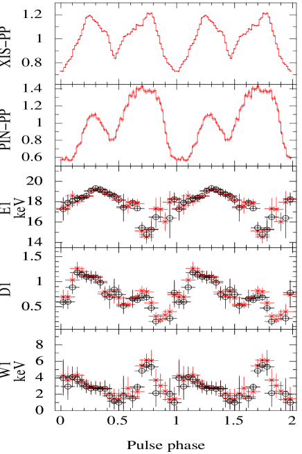
Figure 7: Variation of the cyclotron line parameters in 4U 1907+09 as is obtained with the two models. The black points denotes the parameters as obtained with the ’NPEX’ model The red points denote the parameters as obtained with the ’CompTT’ model. Only 8 of the 25 bins are independent. The XIS (0.3-10 keV) and PIN (10-70 keV)pulse profiles are shown in the top two panels respectively which denote the normalized intensity.

$\begin{array}[]{cc}\includegraphics[height=284.52756pt,width=170.71652pt]{phase-res-0535-npex.ps}&\includegraphics[height=284.52756pt,width=199.16928pt]{phase-res-0535-comptt.ps}\\ \end{array}$

Figure 8: Variation of the spectral parameters with phase along with the pulse profile (0.3-12 keV for XIS and 10-70 keV for PIN) in A 0535+26. The left panel shows the variation using the model ’NPEX’ and the right panel shows the same using the model ’CompTT’. The pulse profiles denote the normalized intensity. The XIS (0.3-10 keV) and PIN (10-70 keV) pulse profiles are shown in the top two panels respectively which denote the normalized intensity.

$\begin{array}[]{cc}\includegraphics[height=284.52756pt,width=170.71652pt]{phase_resres-highecut-1946.ps}&\includegraphics[height=284.52756pt,width=170.71652pt]{phase_res_npex_1946.ps}\\ \end{array}$

Figure 9: Variation of the spectral parameters with phase along with the pulse profile (0.3-12 keV for XIS and 10-70 keV for PIN) in XTE J1946+274. The left panel shows the variation using the model ’highecut’ and the right panel shows the same using the model ’NPEX’.The pulse profiles denote the normalized intensity. The XIS (0.3-10 keV) and PIN (10-70 keV) pulse profiles are shown in the top two panels respectively which denote the normalized intensity.

Table 1: Best fitting phase averaged spectral parameters of A 0535+26, XTE J1946+274 and 4U 1907+09. Errors quoted are for 99 per cent confidence range.

Model	A 0535+26	XTE J1946+274	4U 1907+09
parameters	NPEX  CompTT	highecut  NPEX	NPEX  CompTT
$N_{\mathrm{H1}}^{a}$ ($10^{22}$ atoms $cm^{-2}$)	$0.59\pm 0.02$  $0.31_{-0.03}^{+0.04}$	$1.30\pm 0.028$  $1.27_{-0.04}^{+0.03}$	$1.97\pm 0.01$  $1.62\pm 0.03$
$N_{\mathrm{H2}}^{b}$ ($10^{22}$ atoms $cm^{-2}$)	$3.74_{-0.36}^{+0.25}$  $7.41_{-1.13}^{+1.45}$	$5.86_{-0.82}^{+0.87}$  $9.03_{-1.73}^{+2.72}$	– –
$Cv_{\mathrm{fract}}$	$0.49\pm 0.01$  $0.37\pm 0.02$	$0.27\pm 0.04$  $0.17_{-0.05}^{+0.04}$	– –
PowIndex	–  –	$1.09_{-0.04}^{+0.05}$ –	–  –
E-folding energy (keV)	–  –	$25.57_{-2.26}^{+2.75}$  –	– –
E-cut energy (keV)	– –	$7.02_{-0.29}^{+0.69}$  –	–  –
$powerlaw_{\mathrm{norm}}^{c}$	–  –	$0.021\pm 0.001$  –	– –
$CompTT_{\mathrm{T0}}$ (keV)	– $0.52\pm 0.04$	– –	– $0.47\pm 0.01$
CompTT KT (keV)	– $14.67_{-1.53}^{+2.07}$	– –	– $4.78\pm 0.04$
CompTT $\tau$	– $7.33_{-0.48}^{+0.44}$	– –	– $14.87\pm 0.08$
$CompTT_{\mathrm{norm}}$ c	–  $0.008\pm 0.0009$	– –	– $0.0317\pm 0.0005$
NPEX $\alpha 1$	$1.01_{-0.04}^{+0.05}$  –	– $0.70_{-0.10}^{+0.08}$	$0.84\pm 0.02$ –
NPEX $\alpha 2$	-2.0 (frozen)  –	– -2.0 (frozen)	-2.0 (frozen)  –
NPEX KT (keV)	$11.49_{-1.13}^{+1.56}$  –	– $13.29_{-2.74}^{+2.43}$	$4.41\pm 0.04$  –
$NPEX_{\mathrm{norm}}$ $1^{c}$	$0.041_{-0.001}^{+0.002}$  –	– $0.014_{-0.001}^{+0.002}$	$0.072\pm 0.001$  –
$NPEX_{\mathrm{norm}}$ $2^{c}$	$4.94e-6\pm 1.25e-6$  –	–  $2.34^{d}$ $\pm$ $1.5$	$2.47e-4$ $\pm$ $7.5e-6$  –
$E1_{\mathrm{cycl}}$	$42.60_{-0.84}^{+0.91}$  $43.24_{-0.65}^{+0.85}$	$38.30_{-1.36}^{+1.63}$ $38.65_{-1.76}^{+1.97}$	$17.96_{-0.19}^{+0.20}$  $18.07\pm 0.18$
$D1_{\mathrm{cycl}}$ e	$1.37_{-0.23}^{+0.25}$  $1.43_{-0.26}^{+0.35}$	$1.72_{-0.28}^{+0.41}$  $1.50_{-0.43}^{+0.56}$	$0.68\pm 0.03$  $0.61\pm 0.03$
$W1_{\mathrm{cycl}}$	$7.17_{-1.82}^{+2.28}$  $4.93_{-1.20}^{+1.37}$	$9.61_{-3.06}^{+3.69}$ $8.61_{-3.32}^{+5.45}$	$3.34_{-0.37}^{+0.39}$ $2.78_{-0.37}^{+0.39}$
Iron line energy (keV)	– –	– –	$7.10_{-0.024}^{+0.035}$ $7.10_{-0.037}^{+0.033}$
Iron line eqwidth (eV)	– –	– –	$10.74\pm 2.90$  $7.9\pm 2.6$
Iron line energy (keV)	6.41$\pm$ 0.01  6.41$\pm$ 0.01	$6.41\pm 0.022$  $6.41\pm 0.02$	$6.42_{-0.010}^{+0.008}$  $6.42_{-0.009}^{+0.007}$
Iron line eqwidth (eV)	$23.37\pm 4.61$  $24.28\pm 5.26$	$29.05\pm 4.93$  $28.39\pm 5.15$	$51.67\pm 3.62$  $43.81\pm 1.66$
Flux (XIS) f (0.3-10 keV)	$3.05\pm 0.04$ $3.05\pm 0.05$	$1.80\pm 0.02$  $1.80\pm 0.02$	$4.75\pm 0.06$  $4.74\pm 0.06$
Flux (PIN) g (10-70 keV)	$8.14\pm 0.02$ $8.14\pm 0.03$	$3.47\pm 0.01$ $3.59\pm 0.0$	$6.87\pm 0.02$  $6.91\pm 0.02$
reduced $\chi^{2}$/d.o.f	1.25/839 1.26/837	1.09/826 1.11/826	1.51/837 1.69/838

^a Denotes the Galactic line of sight absorption ^b Denotes the local absorption by the partial covering absorber ’pcfabs’.
^c $\mathrm{photons}\,\mathrm{keV}^{-1}\,\mathrm{cm}^{-2}\,\mathrm{s}^{-1}\,\mathrm{at}\,1\,\mathrm{keV}$
^d $*10^{-7}$ ; ^c denotes the optical depth of the feature.
^e $10^{-10}\,\mathrm{ergs}\,\mathrm{cm}^{-2}\,\mathrm{s}^{-1}$ and are in 99 % confidence range.
^f $10^{-10}\,\mathrm{ergs}\,\mathrm{cm}^{-2}\,\mathrm{s}^{-1}$ and are in 99 % confidence range.

References

- Araya & Harding (1999) Araya, R. A., & Harding, A. K. 1999, ApJ, 517, 334
- Araya-Góchez & Harding (2000) Araya-Góchez, R. A., & Harding, A. K. 2000, ApJ, 544, 1067
- Bartolini et al. (1978) Bartolini, C., Guarnieri, A., Piccioni, A., Giangrande, A., & Giovannelli, F. 1978, IAU Circ., 3167, 1
- Baykal et al. (2006) Baykal, A., İnam, S. Ç., & Beklen, E. 2006, MNRAS, 369, 1760
- Caballero et al. (2007) Caballero, I., Kretschmar, P., Santangelo, A., et al. 2007, A&A, 465, L21
- Caballero et al. (2010a) Caballero, I., Pottschmidt, K., Barragan, L., et al. 2010a, arXiv:1003.2969
- Caballero et al. (2010b) Caballero, I., Pottschmidt, K., Bozzo, E., et al. 2010b, The Astronomer’s Telegram, 2692,
- Caballero et al. (2011a) Caballero, I., Pottschmidt, K., Santangelo, A., et al. 2011a, arXiv:1107.3417
- Caballero et al. (2011b) Caballero, I., Ferrigno, C., Klochkov, D., et al. 2011b, The Astronomer’s Telegram, 3204, 1
- Coburn (2001) Coburn, W. 2001, Ph.D. Thesis, W. A., Rothschild, R. E., et al. 2002, ApJ, 580, 394
- Cox et al. (2005) Cox, N. L. J., Kaper, L., & Mokiem, M. R. 2005, A&A, 436, 661
- Cusumano et al. (1998) Cusumano, G., di Salvo, T., Burderi, L., et al. 1998, A&A, 338, L79
- Davidson & Ostriker (1973) Davidson, K., & Ostriker, J. P. 1973, ApJ, 179, 585
- Enoto et al. (2008) Enoto, T., Makishima, K., Terada, Y., et al. 2008, PASJ, 60, 57
- Finger et al. (2006) Finger, M. H., Camero-Arranz, A., Kretschmar, P., Wilson, C., & Patel, S. 2006, Bulletin of the American Astronomical Society, 38, 359
- Fritz et al. (2006) Fritz, S., Kreykenbohm, I., Wilms, J., et al. 2006, A&A, 458, 885
- Fukazawa et al. (2009) Fukazawa, Y., Mizuno, T., Watanabe, S., et al. 2009, PASJ, 61, 17
- Giacconi et al. (1971) Giacconi, R., Kellogg, E., Gorenstein, P., Gursky, H., & Tananbaum, H. 1971, ApJ, 165, L27
- Giangrande et al. (1980) Giangrande, A., Giovannelli, F., Bartolini, C., Guarnieri, A., & Piccioni, A. 1980, A&AS, 40, 289
- Grove et al. (1995) Grove, J. E., Strickman, M. S., Johnson, W. N., et al. 1995, ApJ, 438, L25
- Heindl et al. (2000) Heindl, W. A., Coburn, W., Gruber, D. E., et al. 2000, American Institute of Physics Conference Series, 510, 173
- Heindl et al. (2001) Heindl, W. A., Coburn, W., Gruber, D. E., et al. 2001, ApJ, 563, L35
- Inam et al. (2009) Inam, S. Ç., Şahiner, Ş., & Baykal, A. 2009, MNRAS, 395, 1015
- in ’t Zand et al. (1997) in ’t Zand, J. J. M., Strohmayer, T. E., & Baykal, A. 1997, ApJ, 479, L47
- in ’t Zand et al. (1998) in ’t Zand, J. J. M., Baykal, A., & Strohmayer, T. E. 1998, ApJ, 496, 386
- Iwakiri et al. (2012) Iwakiri, W. B., Terada, Y., Mihara, T., et al. 2012, ApJ, 751, 35
- Kendziorra et al. (1994) Kendziorra, E., Kretschmar, P., Pan, H. C., et al. 1994, A&A, 291, L31
- Klochkov et al. (2008) Klochkov, D., Staubert, R., Postnov, K., et al. 2008, A&A, 482, 907
- Koyama et al. (2007) Koyama, K., Tsunemi, H., Dotani, T., et al. 2007, PASJ, 59, 23
- Kraus (2001) Kraus, U. 2001, ApJ, 563, 289
- Kretschmar et al. (1996) Kretschmar, P., Pan, H. C., Kendziorra, E., et al. 1996, A&AS, 120, 175
- Kreykenbohm et al. (1999) Kreykenbohm, I., Kretschmar, P., Wilms, J., et al. 1999, A&A, 341, 141
- Kreykenbohm et al. (2002) Kreykenbohm, I., Coburn, W., Wilms, J., et al. 2002, A&A, 395, 129
- Kreykenbohm et al. (2008) Kreykenbohm, I., Wilms, J., Kretschmar, P., et al. 2008, A&A, 492, 511
- La Barbera et al. (2003) La Barbera, A., Santangelo, A., Orlandini, M., & Segreto, A. 2003, A&A, 400, 993
- Lamb et al. (1973) Lamb, F. K., Pethick, C. J., & Pines, D. 1973, ApJ, 184, 271
- Makishima & Mihara (1992) Makishima, K., & Mihara, T. 1992, Frontiers Science Series, 23
- Makishima et al. (1999) Makishima, K., Mihara, T., Nagase, F., & Tanaka, Y. 1999, ApJ, 525, 978
- Maitra et al. (2012) Maitra, C., Paul, B., & Naik, S. 2012, MNRAS, 2231
- Maitra & Paul (2013) Maitra, C., & Paul, B. 2013, ApJ, 763, 79
- Mészáros (1992) Mészáros, P. 1992, High-energy radiation from magnetized neutron stars., by Mészáros, P.. University of Chicago Press, Chicago, IL (USA), 1992, 544 p., ISBN 0-226-52093-5, Price US$ 98.00. ISBN 0-226-52094-3 (paper).,
- Mihara (1995) Mihara, T. 1995, Ph.D. Thesis,
- Mihara et al. (2010) Mihara, T., Yamamoto, T., Sugizaki, M., Nakajima, M., & Maxi Team 2010, The First Year of MAXI: Monitoring Variable X-ray Sources,
- Mitsuda et al. (2007) Mitsuda, K., Bautz, M., Inoue, H., et al. 2007, PASJ, 59, 1
- Mukerjee et al. (2001) Mukerjee, K., Agrawal, P. C., Paul, B., et al. 2001, ApJ, 548, 368
- Mukherjee & Paul (2005) Mukherjee, U., & Paul, B. 2005, A&A, 431, 667
- Mukherjee & Bhattacharya (2012) Mukherjee, D., & Bhattacharya, D. 2012, MNRAS, 420, 720
- Müller et al. (2012) Müller, S., Kühnel, M., Caballero, I., et al. 2012, arXiv:1209.1918
- Nishimura (2008) Nishimura, O. 2008, ApJ, 672, 1127
- Nishimura (2011) Nishimura, O. 2011, ApJ, 730, 106
- Naik et al. (2008) Naik, S., Dotani, T., Terada, Y., et al. 2008, ApJ, 672, 516
- Nakajima et al. (2010) Nakajima, M., Mihara, T., & Makishima, K. 2010, ApJ, 710, 1755
- Negueruela et al. (2000) Negueruela, I., Reig, P., Finger, M. H., & Roche, P. 2000, A&A, 356, 1003
- Paul et al. (2001) Paul, B., Agrawal, P. C., Mukerjee, K., et al. 2001, A&A, 370, 529
- Pottschmidt et al. (2012) Pottschmidt, K., Suchy, S., Rivers, E., et al. 2012, American Institute of Physics Conference Series, 1427, 60
- Pringle & Rees (1972) Pringle, J. E., & Rees, M. J. 1972, A&A, 21, 1
- Robba et al. (2001) Robba, N. R., Burderi, L., Di Salvo, T., Iaria, R., & Cusumano, G. 2001, ApJ, 562, 950
- Rivers et al. (2010) Rivers, E., Markowitz, A., Pottschmidt, K., et al. 2010, ApJ, 709, 179
- Rosenberg et al. (1975) Rosenberg, F. D., Eyles, C. J., Skinner, G. K., & Willmore, A. P. 1975, Nature, 256, 628
- Schönherr et al. (2007) Schönherr, G., Wilms, J., Kretschmar, P., et al. 2007, A&A, 472, 353
- Schwartz et al. (1972) Schwartz, D. A., Bleach, R. D., Boldt, E. A., Holt, S. S., & Serlemitsos, P. J. 1972, ApJ, 173, L51
- Smith et al. (1998) Smith, D. A., Takeshima, T., Wilson, C. A., et al. 1998, IAU Circ., 7014, 1
- Soong et al. (1990) Soong, Y., Gruber, D. E., Peterson, L. E., & Rothschild, R. E. 1990, ApJ, 348, 641
- Suchy et al. (2008) Suchy, S., Pottschmidt, K., Wilms, J., et al. 2008, ApJ, 675, 1487
- Suchy et al. (2011) Suchy, S., Pottschmidt, K., Rothschild, R. E., et al. 2011, ApJ, 733, 15
- Suchy et al. (2012) Suchy, S., Fürst, F., Pottschmidt, K., et al. 2012, ApJ, 745, 124
- Sunyaev & Titarchuk (1980) Sunyaev, R. A., & Titarchuk, L. G. 1980, A&A, 86, 121
- Steele et al. (1998) Steele, I. A., Negueruela, I., Coe, M. J., & Roche, P. 1998, MNRAS, 297, L5
- Tanaka (1986) Tanaka, Y. 1986, IAU Colloq. 89: Radiation Hydrodynamics in Stars and Compact Objects, 255, 198
- Takahashi et al. (2007) Takahashi, T., Abe, K., Endo, M., et al. 2007, PASJ, 59, 35
- Terada et al. (2006) Terada, Y., Mihara, T., Nakajima, M., et al. 2006, ApJ, 648, L139
- Titarchuk (1994) Titarchuk, L. 1994, ApJ, 434, 570
- Truemper et al. (1978) Truemper, J., Pietsch, W., Reppin, C., et al. 1978, ApJ, 219, L105
- Trümper et al. (1977) Trümper, J., Pietsch, W., Reppin, C., & Sacco, B. 1977, Eighth Texas Symposium on Relativistic Astrophysics, 302, 538
- Verrecchia et al. (2002) Verrecchia, F., Israel, G. L., Negueruela, I., et al. 2002, A&A, 393, 983
- White et al. (1983) White, N. E., Swank, J. H., & Holt, S. S. 1983, ApJ, 270, 711
- Wilson et al. (1998) Wilson, C. A., Finger, M. H., Wilson, R. B., & Scott, D. M. 1998, IAU Circ., 7014, 2
- Wilson et al. (2003) Wilson, C. A., Finger, M. H., Coe, M. J., & Negueruela, I. 2003, ApJ, 584, 996
- Yamada et al. (2012) Yamada, S., Uchiyama, H., Dotani, T., et al. 2012, PASJ, 64, 53