Phase separation on a hyperbolic lattice

Abstract

We report a preliminary numerical study by kinetic Monte Carlo simulation of the dynamics of phase separation following a quench from high to low temperature in a system with a single, conserved, scalar order parameter (a kinetic Ising ferromagnet) confined to a hyperbolic lattice. The results are compared with simulations of the same system on two different, Euclidean lattices, in which cases we observe power-law domain growth with an exponent near the theoretically known value of 1/3. For the hyperbolic lattice we observe much slower domain growth, consistent to within our current accuracy with power-law growth with a much smaller exponent near 0.13. The paper also includes a brief introduction to non-Euclidean lattices and their mapping to the Euclidean plane.

Keywords: Hyperbolic lattice; Phase separation; Coarsening; Kinetic Monte Carlo simulation.

I Introduction

The geometry most familiar to condensed-matter physicists is the Euclidean one with its vanishing Gaussian curvature Note1 . The circumference and area of a circle of radius $\rho$ in the Euclidean plane are the well-known power laws, $C(\rho)=2\pi\rho$ and $A(\rho)=\int_{0}^{\rho}C(r)dr=\pi\rho^{2}$, respectively. Almost equally familiar are elliptic or spherical surfaces, exemplified in the macroscopic world by the Earth’s surface and in the nanoscopic world by carbon buckyballs. These closed surfaces have positive Gaussian curvature, $\kappa>0$. Hereafter using dimensionless units such that $|\kappa|=1$, the circular circumference and area are analogously given by $C(\rho)=2\pi\sin\rho$ and $A(\rho)=2\pi(1-\cos\rho)$.

More exotic to most is probably the hyperbolic geometry with its negative Gaussian curvature, $\kappa<0$. In this case the dimensionless circular circumference and area are exponentially divergent: $C(\rho)=2\pi\sinh\rho$ and $A(\rho)=2\pi(\cosh\rho-1)$. The best known example is the Minkowski metric of relativistic spacetime. However, hyperbolic surfaces have recently been studied in nanoscience as well, including junctions of several carbon nanotubes PARK03 and anisotropic lipid membranes GIOM12 . Percolation on hyperbolic lattices has also been studied GU12 .

In this paper we present preliminary results on a comparison of the dynamics of pattern formation during phase separation (spinodal decomposition) in media confined to Euclidean and hyperbolic surfaces. As our example we use an $S=1/2$ ferromagnetic Ising model on a regular lattice embedded in the surface, and we study the time evolution of the characteristic pattern length following a quench from infinite temperature to one well below the model’s critical temperature.

The rest of the paper is organized as follows. In Sec. II we describe the Poincaré disk mapping used to map patterns on a hyperbolic surface onto a Euclidean plane. Next, in Sec. III, we describe the lattices generated by regular tesselations of Euclidean, spherical, and hyperbolic surfaces. The phenomenology of phase separation is briefly reviewed in Sec. IV, and the methods of simulation and data analysis are discussed in Sec. V. Our numerical results are presented in Sec. VI, and a final discussion and suggestions for future work are given in Sec. VII.

II Poincaré disk mapping of non-Euclidean surfaces

Patterns on a non-Euclidean surface cannot be reproduced on a Euclidean surface without distortion; angular, linear, or both. No single rendering is ideal in every respect, as evidenced by the many different geographic map projections developed over the centuries. The projection of the hyperbolic plane that we use in this paper is known as the Poincaré disk mapping and is illustrated in Fig. 1. It consists of a Euclidean plane, a unit sphere ($\kappa=+1$), and a unit hyperboloid of revolution ($\kappa=-1$) CRIA01 . The plane forms the equatorial plane of the sphere, and the hyperboloid rests with its apex on the North Pole of the sphere, (0,1). A straight line through the South Pole, (0,$-1$), connects the points H on the hyperboloid and S on the sphere with their mapping D on the plane. The region of the equatorial plane inside the sphere is the Poincaré disk. It is easily seen from Fig. 1 that an arbitrary point H on the hyperboloid is mapped inside the Poincaré disk, leading in the map to an exponential contraction of lengths far away from the apex of the hyperbola. The mapping from H to D is conformal (angle-preserving), and geodesics on the hyperboloid are mapped onto circles on the disk that meet its edge at straight angles. A little calculus shows that the “hyperbolic radius” of H, $\rho_{\rm H}$, is the arc length of the geodesic from (0,1) to H, calculated with the Minkowski metric, $ds=\sqrt{dx^{2}-du^{2}}$. (Analogously, the “spherical radius” of S, $\rho_{\rm S}$, is the arc length of the geodesic from (0,1) to S, calculated with the Euclidean metric, $ds=\sqrt{dx^{2}+du^{2}}$.) Other equations relevant to the mappings are included in Fig. 1.

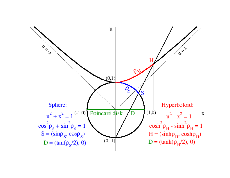
Figure 1: The Poincaré disk mappings from a unit hyperboloid of revolution ($\kappa=-1$) and a unit sphere ($\kappa=+1$) to a Euclidean plane. The $y$ coordinate points into the page and has been suppressed in our notation, describing the position of a point as $(x,u)$. See discussion in Sec. II.

III Euclidean, elliptic, and hyperbolic lattices

To construct lattices embedded in Euclidean and non-Euclidean surfaces, we consider regular tessellations of such surfaces by regular polygons. A lattice created by this procedure, such that $q$ regular $p$-gons meet at every lattice site is characterized by its Schläffli symbol, $\{p,q\}$ GU12 . A lattice of finite size is often denoted by the amended Schläffli symbol, $\{p,q,R\}$, where $R$ is the number of concentric layers of $p$-gons surrounding the central site. The only three regular tessellations of the Euclidean plane are shown in Fig. 2. Any regular $p$-gon can be decomposed into $p$ isosceles triangles that meet at its centroid. This is not only true for Euclidean lattices. An illustration for the hyperbolic case is shown in Fig. 3. Each triangle has apex angle $\theta$ and basal angles $\phi/2$.

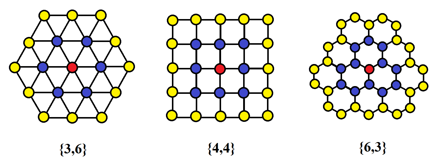
Figure 2: The three regular Euclidean lattices $\{p,q\}$ of $q$ $p$-gons meeting at each lattice site. Here, each is shown with $r=2$ layers of polygons: $\{3,6,2\}$, $\{4,4,2\}$, and $\{6,3,2\}$. The $\{3,6\}$ and $\{6,3\}$ lattices are each other’s duals, while $\{4,4\}$ is self-dual.

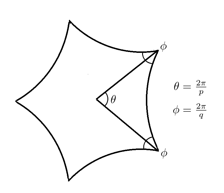
Figure 3: Splitting a hyperbolic pentagon into five isosceles triangles.

For the Euclidean plane, the interior angles of a triangle must always sum to $\pi$. Thus,

$$2\pi/p+2\pi/q=\pi\Leftrightarrow(p-2)(q-2)=4\;.$$ (1)

This proves that the only combinations of integer $p$ and $q$ compatible with Euclidean geometry are $\{3,6\}$, $\{4,4\}$, and $\{6,3\}$.

Similarly, for the elliptic plane,

$$2\pi/p+2\pi/q>\pi\Leftrightarrow(p-2)(q-2)<4\;.$$ (2)

Again it is clear that the number of possible regular tessellations is finite. In fact, they correspond to the five Platonic solids, $\{3,3\}$, $\{3,4\}$, $\{3,5\}$, $\{4,3\}$, and $\{5,3\}$ COXE63 .

For the hyperbolic plane, on the other hand,

$$2\pi/p+2\pi/q<\pi\Leftrightarrow(p-2)(q-2)>4\;.$$ (3)

Consequently, the number of possible regular tessellations is infinite. Some examples are shown in Figs. 4 and 5. As the size of the lattice increases, embedding without overlaps into a three-dimensional Euclidean space becomes impossible. Fascinating images of models of hyperbolic planes created by crocheting can be found in Ref. TAIM09 .

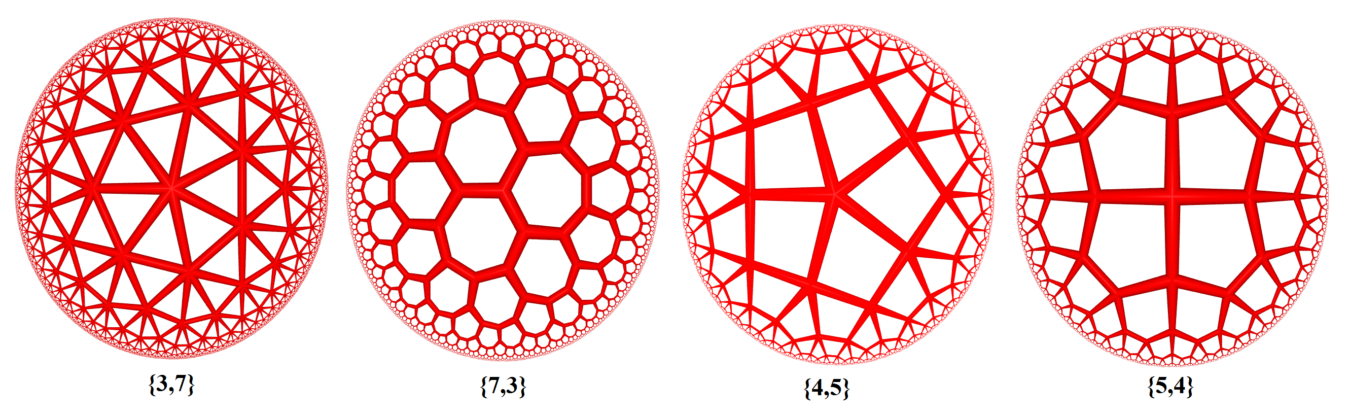
Figure 4: Some examples of the infinite number of hyperbolic lattices, projected onto the Poincaré disk. The exponential length contraction in the projected image of large $\rho_{\rm H}$ is clearly evident. As for the Euclidean and elliptic geometries, $\{p,q\}$ and $\{q,p\}$ are duals.

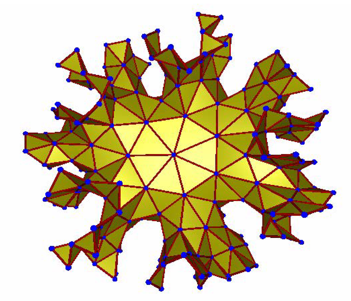
Figure 5: Perspective image of a small $\{3,7,4\}$ lattice embedded in a three-dimensional Euclidean space. The exponential divergence of the hyperbolic circumference with radius prohibits such embedding without overlaps for large lattices.

IV Phase separation

Phase separation occurs when a binary mixture is quenched from a high temperature into the phase-coexistence region below its critical temperature. As coherent regions of the two coexisting phases form and grow after the quench, the length scale characterizing the typical domain size increases algebraically with time as

$$\xi\sim t^{n}\;.$$ (4)

The growth exponent $n$ depends on the symmetries and conservation laws governing the dynamics. For the case of two-phase coexistence and a constant ratio of the volumes of the two phases, $n=1/3$. This situation is known in the terminology of critical dynamics as Lifshitz-Slyozov dynamics LIFS62 or Model B HOHE77 . However, these results implicitly assume a Euclidean geometry, and we are not aware that the prediction has yet been tested in the hyperbolic case. A numerical test is the purpose of the work presented here.

V Simulation and data analysis

We consider the phase separation that occurs when a $S=1/2$ Ising ferromagnet with spins $s_{i}=\pm 1$ placed at the vertices of the $\{p,q\}$ lattice is quenched from a high temperature to one well below its critical temperature. The Hamiltonian is given by

$${\mathcal{H}}=-J\sum_{\langle i,j\rangle}s_{i}s_{j}\;.$$ (5)

Here, $J>0$ is the ferromagnetic interaction constant, and the sum runs over all nearest-neighbor pairs. The coordination number in a $\{p,q\}$ lattice is $q$. We will use units such that Boltzmann’s constant and $J$ both equal unity.

While the phase transition at the critical temperature $T_{c}$ for this model on Euclidean lattices belongs to the two-dimensional Ising universality class, on hyperbolic lattices it belongs to the mean-field universality class KRCM08 ; GEND12 . In either case, the value of $T_{c}$ increases with $q$. ($T_{c}=2/\ln(1+\sqrt{2})\approx 2.269$ for $\{4,4\}$, $4/\ln 3\approx 3.641$ for $\{3,6\}$, and $\approx 5.5$ for $\{3,7\}$ GEND12 .) To minimize surface effects, we use periodic boundary conditions for the two Euclidean lattices. Unfortunately we are not aware of a method for doing so in the hyperbolic case, and consequently we simulate the $\{3,7\}$ lattice with free boundary conditions.

The initial state is a random distribution of up and down spins, subject only to the constraint of a vanishing order parameter, $\sum_{i}s_{i}=0$. The time evolution is obtained from a kinetic Monte Carlo (MC) simulation by the order-parameter conserving Kawasaki dynamics KAWA72 . This algorithm consists in randomly choosing a nearest-neighbor spin pair and checking if the two spins are different. If they are equal, a different pair is chosen. If the spins are different, they are exchanged with the Metropolis probability,

$$P_{\rm ex}(s_{i},s_{j})=\min[1,\exp(-\Delta E/T)]\;,$$ (6)

where $\Delta E$ is the energy change that would result from a successful spin exchange. In a system consisting of $N$ spins, $N$ random choices of a spin pair constitute the MC time unit, one MC step per spin (one MCSS). Snapshots of the $\{3,6\}$ and $\{3,7\}$ lattices in their initial, disordered states and at $t=10^{6}$ MCSS, when macroscopic bulk phase domains are well developed, are shown in Fig. 6.

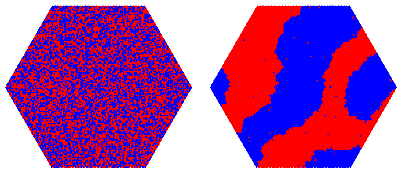
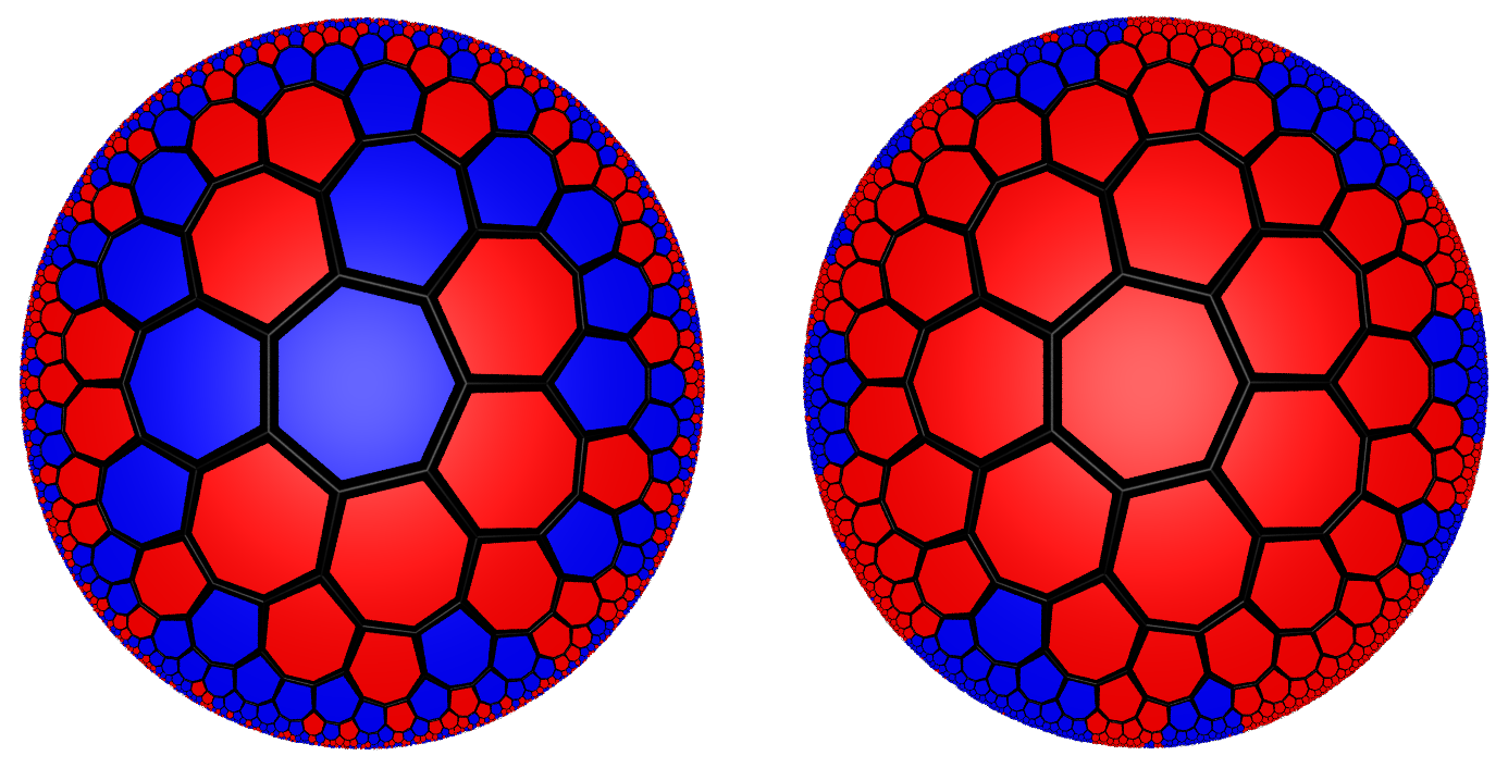
Figure 6: Snapshots of the $\{3,6,60\}$ (left) and $\{3,7,8\}$ lattices (right) in their initial, disordered states and at times near the end of the simulation runs. $T=2.0$, in both cases well below $T_{c}$. Small thermal fluctuations in the bulk phases are noticeable for the $\{3,6\}$ case.

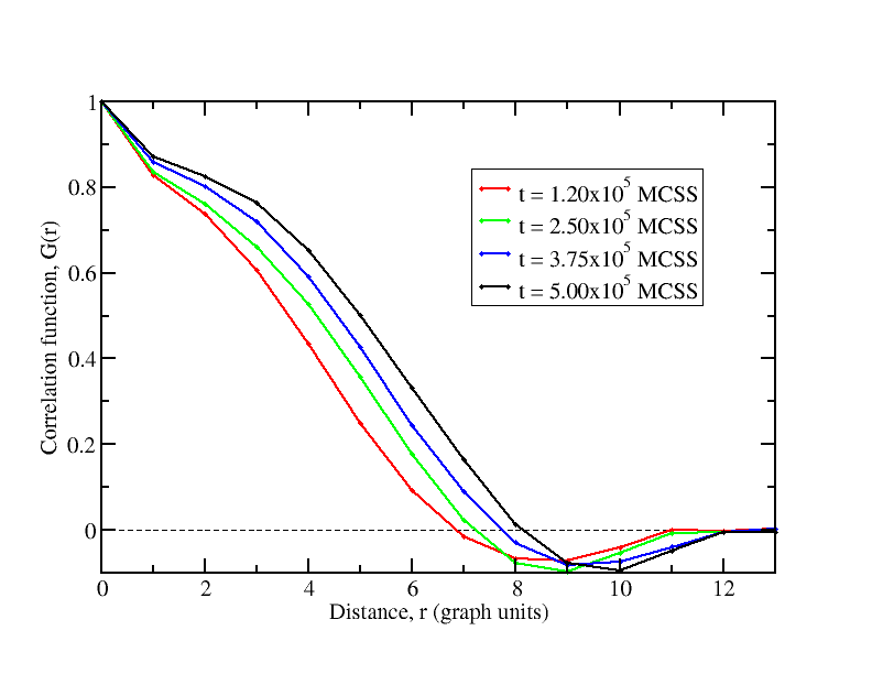
Figure 7: The spin correlation function $G(r)$ for a $\{3,7,7\}$ lattice at different times. The correlation length $\xi(t)$ is estimated as the distance corresponding to the first zero crossing of $G(r)$, as discussed in the text.

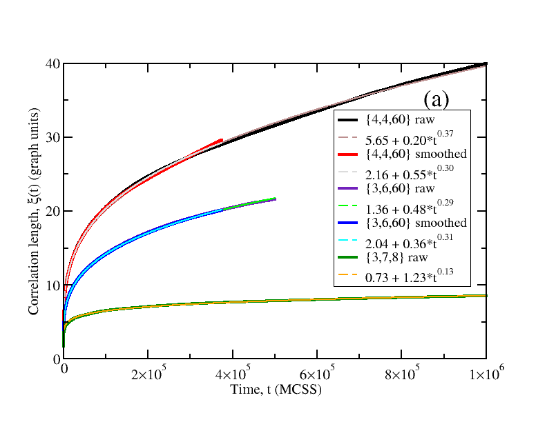
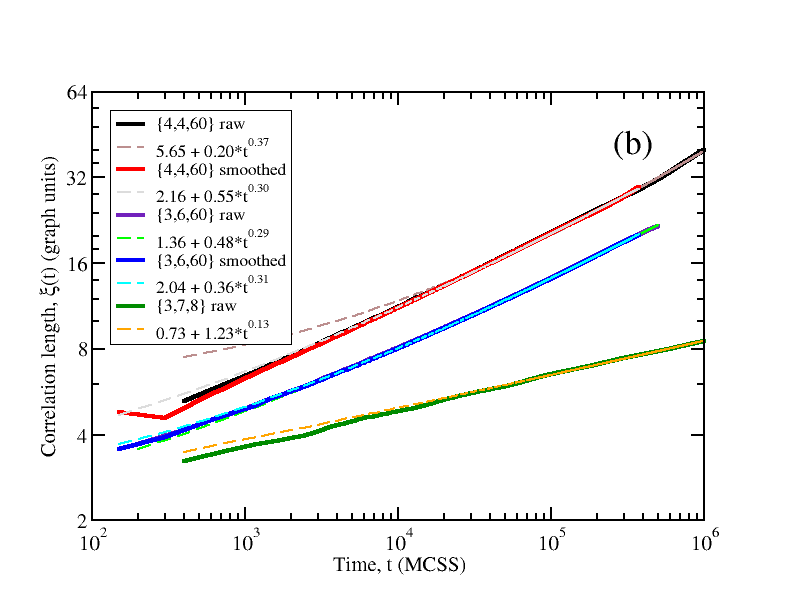
Figure 8: Simulation data for the correlation length $\xi$ (solid curves), together with three-parameter nonlinear fits (dashed curves), shown versus time $t$ for lattices $\{4,4,60\}$ (14,400 sites), $\{3,6,60\}$ (10,800 sites), and $\{3,7,8\}$ (11,173 sites). Linear scale (a) and log-log scale (b). In the legends, “raw” refers to data not corrected for thermal fluctuations, and “smoothed” refers to data with thermal fluctuations filtered out as discussed in the text. The filtered data give an estimate of the growth exponent of $n\approx 0.3$ for the Euclidean lattices, compatible with the theoretical value $n=1/3$. However, the effective exponent obtained for the hyperbolic lattice is much lower: approximately 0.13.

The power-law result for the characteristic length scale given in Eq. (4) assumes an isotropic system with sharp interfaces and no thermal fluctuations in the bulk phase regions. Neither assumption is well satisfied for discrete Ising models at nonzero temperature. Care must therefore be exercised in extracting the relevant, growing length scale from the simulated spin configurations. Here we calculate the two-point correlation function, $G(r)=\langle s(r_{i})s(r_{i}+r)\rangle$, where $r_{i}$ is the position of lattice point $i$, and $r_{i}+r$ is the position of a lattice point a distance $r$ away from $i$. Here, $r$ is defined as the shortest path between two lattice points along the edges (“taxicab” or “Manhattan” distance). The correlation length $\xi(t)$ is estimated as the first zero crossing of $G(r)$ at time $t$. See Fig. 7. To reduce the effect on the estimate of thermal fluctuations in the bulk phases, we perform the simulations at relatively low temperatures, compared to $T_{c}$. In calculating the correlation functions we also ignore isolated single spins and spin pairs MAJU10 , which otherwise could distort $G(r)$ for $r=1$ and 2, as seen in Fig. 7.

VI Numerical results

The main numerical results of this study are summarized in Figs. 8 and 9. Figure 8 shows the length scale $\xi$ as a function of time for each of the three studied lattices, following a quench to $T=2.0$. The data sets were averaged over 1,500 independent simulation runs for the Euclidean lattices, and 1000 runs for the hyperbolic lattice. Results are included, both based on the raw data, and with thermal fluctuations filtered out as discussed above. Significant differences are only observed for $\{4,4\}$, for which the quench temperature is not very far below $T_{c}$. The growth exponents are here estimated by three-parameter, nonlinear fits to the time series, with the results given in the figure legends. For both the Euclidean lattices, the growth exponent comes out as $n\approx 0.3$, consistent with the expected value of $1/3$. For the hyperbolic $\{3,7\}$ lattice, however, the effective exponent is significantly lower, only about 0.13.

In Fig. 9 we show results obtained by a different way of estimating the exponents. The data were divided into bins, each containing twice as many data points as the previous one (“octave binning”). We then performed a linear least-squares fit to $\log_{10}\xi$ versus $\log_{10}t$ in each successive pair of bins. Subtraction of a constant background was adjusted so that the estimated exponents became roughly independent of $t$. The resulting exponent estimates are seen to be consistent with those obtained by nonlinear fitting over the entire time interval.

It is reasonable to ask whether the much lower effective growth exponent obtained for the hyperbolic lattice might be a result of finite-size saturation of the length scale. To check this possibility, we also performed simulations for smaller $\{3,7\}$ lattices with $R$ between 3 and 6. As seen in Fig. 10, saturation does not appear to set in earlier than $10^{6}$ MCSS, even for a system as small as $R=6$.

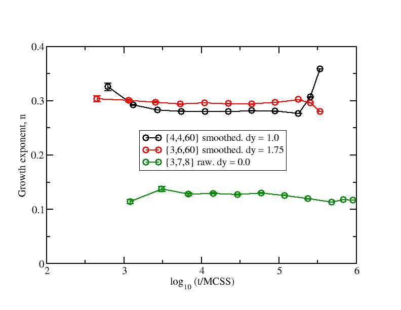
Figure 9: Estimates of the growth exponent $n$, based on the moving least-squares averaging method described in the text. The average values obtained are 0.30 for the two Euclidean lattices, and 0.12 for the hyperbolic $\{3,7\}$ lattice. These values are consistent with the ones obtained by nonlinear fitting and shown in Fig. 8. $dy$ refers to the constant background subtraction applied to the data to obtain exponent estimates approximately independent of $t$.

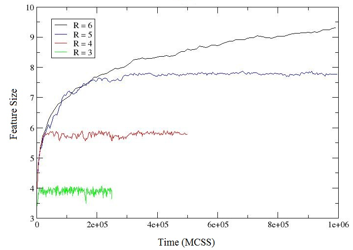
Figure 10: Correlation length $\xi$ versus time for $\{3,7\}$ lattices with $R=3$,…, 6. These results indicate that the low value of the effective growth exponent observed with $R=8$ (see Figs. 8 and 9) is genuine and not due to finite-size saturation of the domain size within the simulation time of $10^{6}$ MCSS.

VII Discussion

Here we have reported a preliminary, numerical investigation of the dynamics of phase separation in a model with a single, conserved, scalar order parameter (Model B) confined to the vertices of a lattice obtained as a regular tiling of a hyperbolic plane. The results are compared with those obtained for the same model on two different Euclidean lattices. The latter show power-law domain growth with an exponent of approximately 0.3, near the theoretical result of 1/3, which is valid for the limiting case of an isotropic continuum system at zero temperature. Considering that the simulations were performed for anisotropic, discrete systems at a finite temperature, this agreement is convincing.

However, for the hyperbolic $\{3,7\}$ lattice with $R$ up to 8, we observe much slower growth, consistent with a power law with an effective exponent of about 0.13. Whether or not this is indeed power-law growth or something else, we leave open for future, theoretical investigation. The effect is possibly related to the fact that for large $R$, most of the spins are located near the free surface. It may also be related to the mean-field nature of the phase transition at $T_{c}$ in the hyperbolic case, which indicates the existence of effective long-range interactions.

For the future we also leave a numerical investigation of phase ordering with non-conserved order parameter (Model A HOHE77 ) on hyperbolic lattices. In this case, the growth exponent in the Euclidean case is known to be 1/2.

References

- (1) As a reminder, the Gaussian curvature of a surface is the product of its two principal curvatures.
- (2) N. Park, M. Yoon, S. Berber, J. Ihm, E. Osawa, D. Tománek, Magnetism in all-carbon nanostructures with negative Gaussian curvature, Phys. Rev. Lett. 91 (2003) 237204.
- (3) L. Giomi, Hyperbolic interfaces, Phys. Rev. Lett. 109 (2012) 136101.
- (4) H. Gu, R. M. Ziff, Crossing on hyperbolic lattices, Phys. Rev. E 85 (2012) 051141.
- (5) C. Criado, N. Alamo, A link between the bounds on relativistic velocities and areas of hyperbolic triangles. Am. J. Phys. 69 (2001) 306-310.
- (6) H. S. M. Coxeter, Regular Polytopes, Dover, New York, 1963.
- (7) D. Taimina, Crocheting adventures with hyperbolic planes, A. K. Peters, Ltd., Wellesley, MA, 2009.
- (8) I. M. Lifshitz, Kinetics of ordering during second-order phase transitions, Sov. Phys. JETP 15 (1962) 939-942.
- (9) P. C. Hohenberg, B. Halperin, Theory of dynamic critical phenomena, Rev. Mod. Phys. 49 (1977) 435-479.
- (10) R. Krcmar, A. Gendiar, K. Ueda, T. Nishino, Ising model on a hyperbolic lattice studied by the corner transfer matrix renormalization group method, J. Phys. A: Math. Gen. 41 (2008) 125001.
- (11) A. Gendiar, R. Krcmar, S. Andergassen, M. Danska, T. Nishino, Weak correlation effects in the Ising model on triangular-tiled hyperbolic lattices, Phys. Rev. E 86 (2012) 021105.
- (12) K. Kawasaki, Kinetics of Ising models, In: C. Domb and M. Green (Ed.), Phase transitions and critical phenomena, Vol. 2, Academic Press, London, 1972.
- (13) S. Majumder, S. K. Das, Domain coarsening in two dimensions: Conserved dynamics and finite-size scaling, Phys. Rev. E 81 (2010), 050102.