A comprehensive picture of baryons in groups and clusters of galaxies

Abstract

Aims. Based on XMM-Newton, Chandra, and SDSS data, we investigate the baryon distribution in groups and clusters and its use as a cosmological constraint. For this, we considered a sample of 123 systems with temperatures ${\rm kT_{500}}=1.0-9.0$ keV, total masses in the mass range ${\rm M_{500}=(\sim 10^{13}-4\times 10^{15})\ h_{70}^{-1}\ M_{\odot}}$, and redshifts 0.02 $<z<$1.3.

Methods. The gas masses and total masses are derived from X-ray data under the assumption of hydrostatic equilibrium and spherical symmetry. The stellar masses are based on SDSS-DR8 optical photometric data. For the 37 systems out of 123 that had both optical and X-ray data available, we investigated the gas, stellar, and total baryon mass fractions inside $r_{2500}$ and $r_{500}$ and the differential gas mass fraction within the spherical annulus between $r_{2500}$ and $r_{500}$, as a function of total mass. For the other objects, we investigated the gas mass fraction only.

Results. We find that the gas mass fraction inside $r_{2500}$ and $r_{500}$ depends on the total mass. However, the differential gas mass fraction does not show any dependence on total mass for systems with ${\rm M_{500}>10^{14}M_{\odot}}$. The stellar mass fraction inside $r_{2500}$ and $r_{500}$ increases towards low-mass systems more steeply than the $f_{\rm gas}$ decrease with total mass. Adding the gas and stellar mass fractions to obtain the total baryonic content, we find it to increase with cluster mass, reaching the WMAP-7 value for clusters with ${\rm M_{500}\sim 10^{14}M_{\odot}}$. This led us to investigate the contribution of the intracluster light to the total baryon budget for lower mass systems, but we find that it cannot account for the difference observed.

Conclusions. The gas mass fraction dependence on total mass observed for groups and clusters could be due to the difficulty of low-mass systems to retain gas inside the inner region ($r<r_{2500}$). Because of their shallower potential well, non-thermal processes are more effective in expelling the gas from their central regions outwards. Since the differential gas mass fraction is nearly constant, it provides better constraints for cosmology. Moreover, we find that the gas mass fraction does not depend on redshift at a $2\sigma$ level. Using our total $f_{\rm b}$ estimates, our results imply $\Omega_{\rm m}<0.55$, and taking the highest significant estimates for $f_{\rm b}$, $\Omega_{\rm m}>0.22$.

1 Introduction

Considering the hierarchical scenario of structure formation, the groups we observe today are the building blocks of future galaxy clusters. Although they collapse and merge to form progressively larger systems, the observations of groups of galaxies show that they are not the scaled-down version of galaxy clusters (e.g., Mulchaey, 2000; Ponman et al., 2003; Voit, 2005). Cluster scaling relations (e.g. the L–T relation) show deviations from self-similar relations at the low-mass end (e.g., Voit, 2005, but see also Eckmiller et al. (2011)), providing evidence of the importance of baryon physics.

Since galaxy groups are cooler with shallower potential wells, non-gravitational processes (e.g., galactic winds, cooling, active galactic nucleus feedback, etc.) play a more significant role in less massive systems. Also, the matter composition in groups is different from that in clusters. Baryons in galaxy groups and clusters can be divided into two major components, the hot gas between galaxies and the stars in galaxies. A minor component is the intra-cluster light. In clusters, the gas is the baryon-dominant component (about 6 times more massive than the stellar mass). While in groups, the gas mass is significantly lower: it is of the same order as the stellar mass (e.g., Laganá et al., 2011) and in some cases, even lower than the stellar component (e.g., Giodini et al., 2009). The analysis of both components is critical for observational cosmology when using groups and clusters to constrain the $\Omega_{m}$ parameter from the observed baryon mass fraction (e.g., Allen et al., 2002; Vikhlinin et al., 2009).

The total baryon mass fraction is defined as the ratio between the gas+stars and the total mass: $f_{\rm b}=(M_{\rm gas}+M_{\rm star})/M_{\rm tot}$. In very massive galaxy clusters ($M_{500}\sim 10^{15}M_{\odot}$), the baryon content is supposed to closely match the Seven-year Wilkinson Microwave Anisotropy Probe (WMAP-7) value ($f_{\rm b}^{\rm WMAP-7}=0.169\pm 0.009$, Jarosik et al., 2011). However, it is found that the total baryon mass fraction (and the gas mass fraction) decreases towards low-mass systems (e.g., Lin et al., 2003; Gonzalez et al., 2007; Giodini et al., 2009; Sun et al., 2009; Laganá et al., 2011; Zhang et al., 2011; Sun, 2012), when analyzing a wide range of masses. On the other hand, the stellar mass fraction seems to increase from clusters to groups of galaxies. A straightforward interpretation can be that the gas mass fraction is directly related to cooling and to the star formation rate, and thus, a smaller gas mass fraction in groups may be related to an efficient cooling. However, the gas mass fraction can also be affected by AGN feedback, which, as mentioned before, is more significant in groups than in clusters. As shown in recent numerical simulations performed by Puchwein et al. (2010), the amount of gas removed by AGN heating from the central regions of clusters and are driven outwards ($r>r_{500}$) depends on cluster mass and is higher in low-mass systems.

The baryon fraction in clusters and groups is an important cosmological probe (e.g., Allen et al., 2004), and therefore scaling relations, such as $f_{\rm gas}$–kT or $f_{\rm gas}$–M500, need to be well understood if we want to use them as a cosmological tool. We will explore here the baryon distribution in the form of gas and stellar mass fractions in groups and compare them with the observed baryon fractions observed in clusters. We will consider in particular the baryon fractions inside the characteristic radii $r_{2500}$ and $r_{500}$, which are commonly observed with the present generation of X-ray telescopes.

Previous works have presented an analysis of the gas fraction in groups, but few have measured the gas properties up to $r_{500}$: Vikhlinin et al. (2006) and Gonzalez et al. (2007) derived the gas mass fraction within $r_{500}$ for four low-temperature systems. Sun et al. (2009) determined gas properties up to $r_{500}$ for 11 out of 43 groups. In groups of galaxies, the stellar mass is of the order of the gas mass. To understand the dependence of the total baryon fraction on total mass, it is important to compute both components, the stellar and gas mass fractions, in a homogeneous way. We thus present here the analysis of nine galaxy groups based on XMM-Newton and Sloan Digital Sky Survey (SDSS DR8) data, for which we could reliably measure gas properties up to $r_{500}$. We also included 114 galaxy clusters from Maughan et al. (2012, hereafter M12) to investigate the gas mass component inside $r_{2500}$ and $r_{500}$, and for 28 of these 114 clusters, we could also estimate the stellar mass fraction.

The paper is organised as follows. The sample is described in Section 2. The data reduction is divided in two sections: Section 3 describes the SDSS-DR8 data reduction, the colour-magnitude diagrams (CMD) constructed to select group galaxies, and the procedure to compute the stellar masses; Section 4 describes the X-ray analysis, gas estimates, and total mass estimates. In Section 5, we present our results and compare them to previous results, which are finally summarized in Sect. 7. A $\Lambda$CDM cosmology with $H_{0}=70\ \rm km\ s^{-1}\ Mpc^{-1}$ and $\Omega_{M}=0.3$ is adopted throughout, and all errors are quoted at the 68% confidence level.

2 The sample

To analyse the baryon mass fraction dependence (gas and stellar mass) on total cluster mass, it is important to consider a sample that covers a wide range of mass, and the objects must have optical and X-ray masses available.

In the present work, we analyse the sample of 114 clusters from Maughan et al. (2008), which were updated in M12, in the redshift range $0.11<z<1.3$ and with temperatures ranging from 2.0 keV up to 8.9 keV. 28 out of 114 have optical data available.

To complete our analysis, we also included nine low-mass systems, which were selected as follows. We first selected all groups with available XMM-Newton and SDSS-DR8 data, imposing an X-ray flux limit of $L_{X}=1.9\times 10^{43}\rm erg/s$, which corresponds to $kT\sim 2\ \rm keV$ (Eckmiller et al., 2011). We had 19 groups (without considering the Hickson groups, which are very particular) fulfilling these conditions. However, nine out of 19 had very shallow X-ray observations (low exposure times) that did not allow us to constrain the gas mass. For this reason, we had to exclude those groups. Another group was on the border of the X-ray detector, so it was excluded too.

We ended with a large sample of 123 systems (0.02$<z<$1.3) with total masses between $10^{13}M_{\odot}$ and $4\times 10^{15}M_{\odot}$. These groups and clusters are listed in Tab. LABEL:tab:geral. We emphasize that we analysed a sample of nine groups and 28 clusters for the total baryon budget. For the gas mass fraction analysis, we worked with 9 groups and 114 clusters from M12. Thus, the sample is mainly composed by clusters in the latter part.

3 Optical data analysis and stellar mass determination

In this section we describe the method adopted to compute the total stellar mass (in galaxies) for our nine groups of galaxies and 28 galaxy clusters from M12. To be homogeneous,the procedure adopted in this work was the same for groups and clusters, and we followed the steps described in Giodini et al. (2009) and Bolzonella et al. (2010) that consider statistical membership, background correction, and mass completeness as a function of redshift, and a geometrical correction.

We used SDSS-DR8 data, from $DERED$ magnitude tables (already corrected for internal galaxy extinction) for all sources in the $GALAXY$ catalog. The $GALAXY$ catalogue is essentially complete down to 21.3 i-magnitude (SDSS-DR7 summary).

To obtain stellar masses, we first transformed apparent magnitudes to absolute magnitudes with the distance modulus, assuming K-correction values, K(z), according to the morphological type (tables from Poggianti, 1997):

$$M=m-25-5\log(d_{L}/1Mpc)-K(z),$$ (1)

where, $d_{L}$ is the luminosity distance.

Absolute magnitudes are converted to luminosities, assuming an absolute magnitude of 4.58 for the Sun in the i-band (Blanton et al., 2003). Luminosities are then converted to masses assuming two different mass-to-light ratios (from Kauffmann et al., 2003): $(M/L_{i})_{\star}=0.74\ M_{\odot}/L_{\odot}$ for late-type and $(M/L_{i})_{\star}=1.70\ M_{\odot}/L_{\odot}$ for early-type galaxies, as described in Laganá et al. (2008). All morphological classification used here is based on the galaxy distribution in a colour-magnitude diagram (CMD), as explained below. Thus, morphological type simply means “early” or “late” type galaxies.

3.1 Completeness

To compare the stellar masses of groups and clusters, we defined the completeness in stellar mass ($\mathcal{M}_{\rm lim}^{\rm star}$), or galaxy absolute magnitude, as a function of redshift (as adopted in Giodini et al., 2009; Bolzonella et al., 2010; Pozzetti et al., 2010). This is the lowest mass at which the galaxy stellar mass function can be considered as reliable and unaffected by incompleteness.

For each galaxy, we computed the “limiting mass”, which is the stellar mass that this galaxy would have if its apparent magnitude was equal to the sample limit magnitude (i.e., i=21.3): $\log\mathcal{M}_{\rm lim}^{\rm star}=\log\mathcal{M}+0.4\times(i-21.3)$, where $\mathcal{M}$ is the stellar mass of the galaxy with apparent magnitude $i$. We then computed this value in small redshift bins by considering the 20% faintest galaxies (the grey points in Fig. 1), that is, those contributing to the faint-mass end of the galaxy stellar mass function. For each redshift bin, we define the value corresponding to 95% of the distribution of limiting masses as a minimum mass. The systems were divided into four bins of redshift, and we fit the limiting mass values as a function of redshift: $\log\mathcal{M}_{\rm lim}^{\rm star}(z)=11.67\times z^{0.13}$ (the red line in Fig. 1). We thus adopted $\mathcal{M}_{\rm lim}^{\rm star}$ as the lowest galaxy stellar mass that will be considered in our analysis to compute the stellar masses for the groups and clusters. As a check, we also computed the theoretical values for the limiting mass, assuming no K-correction and a constant value for the mass-to-light ratio as $\log\mathcal{M}_{\rm lim}^{\rm star}\propto DM(z)/2.5$, where DM is the distance modulus. We see that the adopted function for the limiting mass (red line in Fig. 1) is close to the theoretical predicted value for $\mathcal{M}_{\rm lim}^{\rm star}$ (blue-dashed line in Fig. 1).

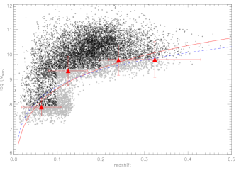
Figure 1: Stellar mass completeness for our system, which is computed from the fit (red line) to the 95% percentile of the distribution in the limiting mass, for galaxies in the 20% lower percentile in magnitude (grey points) as a function of redshift. The black points represent all galaxies inside $r_{\rm 500}$ in the photometric redshift range with $i<21.3$. The blue-dashed line represents the theoretical value, assuming no K-correction and a constant value for the mass-to-light ratio, as stated in the text.

We estimated the contribution from galaxies that are less massive than $\mathcal{M}_{\rm lim}$ in each redshift bin. We assumed that the fraction of galaxies that are not are not considered is $f=1-[\mathcal{M_{\rm star}}(\mathcal{M}>\mathcal{M}_{\rm lim})/\mathcal{M}_{\rm star_{\rm tot}}]$ and can be estimated using a stellar mass function. Thus,

$$f=1-\frac{\int_{\mathcal{M}_{\rm lim}}^{\mathcal{M}_{\rm max}}\mathcal{M}f(\mathcal{M})d\mathcal{M}}{\int_{\mathcal{M}_{\rm min}}^{\mathcal{M}_{\rm max}}\mathcal{M}f(\mathcal{M})d\mathcal{M}},$$ (2)

where $\mathcal{M}_{\rm lim}$ is the limiting mass values for each redshift bin defined by the red points in Fig. 1, and $\mathcal{M}_{\rm min}$ and $\mathcal{M}_{\rm max}$ are the minimum and maximum mass values for the stellar mass in cluster galaxies, respectively. We assumed that $\mathcal{M}_{\rm min}=10^{8}M_{\odot}$ and $\mathcal{M}_{\rm max}=10^{13}M_{\odot}$. Considering that the stellar mass function is described by a single Schechter function, we used typical values from Bell et al. (2003) ($M^{\ast}=10^{6}/h^{2}$, $\alpha=-0.6$) to estimate the fraction of stellar mass that is missing in each redshift bin because of completeness correction. We found that the fractional contribution to the total stellar mass budget of galaxies with $10^{8}M_{\odot}<\mathcal{M}<\mathcal{M}_{\rm lim}(z)$ varies from less than 1% up to 4% (for clusters with $z>0.3$). These small fractions (also in agreement with Lin et al., 2003; Giodini et al., 2009) show that the stellar masses computed in this work are reliable.

3.2 Statistical membership, background correction and geometrical correction

As a first step to estimate the projected total stellar mass, which is the sum of all potential member galaxies (with masses greater than the limiting mass), we first have to define candidate members inside $r_{2500}$ and $r_{500}$. Those members are defined as all the galaxies inside a projected distance equal to $r_{2500}$ or $r_{500}$, which is defined from the X-ray centroid of a group/cluster and with photometric redshift in the range $z=z_{\rm c}\pm 0.1\times(1+z_{\rm photo}^{\rm SDSS})$ (where $z_{c}$ is the central redshift taken from NED, and $z_{\rm photo}^{\rm SDSS}$ is the photometric redshift taken from SDSS-DR8). We note that we used a range of 0.1, which is of the order of the error on photometric redshifts in the SDSS catalogue.

We constructed CMD for each group/cluster to identify the red-sequence. For each system, we linearly fit the red-sequence (RS) and considered all galaxies within the RS best-fit $\pm 0.3$ mag as early-type objects. Late-type galaxies were classified as the objects that are bluer than the lower limit of the RS. We summed the masses of all the early-type and late-type galaxies that obeyed our criteria.

We corrected for background/foreground contamination by measuring the total stellar mass of early-type and late-type galaxies, assuming the same photometric redshift criterium, in an annulus of inner and outer radii of $8\times r_{500}$ and $9\times r_{500}$, respectively (as already described in Lin et al., 2003; Laganá et al., 2008). We applied early- and late-type definitions of the cluster to the background region. Thus, field galaxies are selected by following the same criteria as group/cluster potential members. The background regions do not overlap other structures and were chosen to represent a field environment. We then summed the masses of all late- and early-type galaxies in the background area.

Finally, we added up the stellar masses of all early-type galaxies from our systems and subtracted the stellar masses of background early-type galaxies normalised to the cluster area. The same was done for late-type galaxies. To compute the total stellar mass of the system, we summed the total corrected values for early- and late-type stellar masses, considering our limiting mass for the cluster/groups redshift.

There is one last correction to be applied. The values derived for the stellar masses refer to a cylinder section projected perpendicularly to the line of sight. On the other hand, the gas and total masses are measured inside spheres of radii, $r_{2500}$ and $r_{500}$. To compare stellar masses to total and gas masses, we need to apply a geometrical correction to correct the cylindrical volume to a spherical volume (see Appendix B for more details). The concentration parameters are taken to be 2$\pm$1 and 3$\pm$1 for clusters and groups, respectively. These values lead to a multiplicative factor on the stellar mass of 0.68 for clusters and 0.74 for groups within $r_{500}$ and 0.53 for clusters and 0.61 for groups within $r_{2500}$. One can note that the concentration parameter of clusters is chosen to be lower than the parameter of groups, according to results from Hansen et al. (2005).

3.3 Uncertainties

We have three major uncertainties: the photometric magnitude uncertainty (about 14% of the stellar mass), the uncertainty arising from the geometrical correction (about 6% within $r_{500}$ and 9% within $r_{2500}$), and the uncertainty on the mass to light ratio (about 26%). The error bars are approximated to be the quadrature sum of the three uncertainties, i.e., about 30%. The uncertainty on the geometrical correction has been calculated, assuming the concentration parameter is known at $\pm$1. In most cases, our error bars are mainly because of the uncertainty on the mass-to-light ratio. Thus, it could improve with better constraints on mass-to-light ratios. It is also interesting to note that errors are of the same order within $r_{2500}$ and $r_{500}$, which shows there are enough galaxies within $r_{2500}$ to calculate statistical uncertainties. Stellar masses with error bars are given in Tab. LABEL:tab:geral.

4 X-ray data analysis, gas and total mass determinations

For the nine groups of our sample, we reduced the X-ray data with the XMM-Newton Science Analysis System (SAS) v11.0 and calibration database using all the updates available prior to February 2012. The initial data screening was applied using recommended sets of event patterns - i.e., 0-12 and 0-4 for the MOS and PN cameras, respectively. The light curves in the energy range of [1-10] keV were filtered to reject periods of high background. We used the background maps for the 3 EPIC instruments from Read & Ponman (2003). The background was normalised with a spectrum obtained in an annulus (between 9-11 arcmin), where the cluster emission is no longer detected. A normalised spectrum was then subtracted, yielding a residual spectrum. This normalisation parameter was then used in the spectral fit. This procedure was already adopted in Laganá et al. (2008) and Durret et al. (2010, 2011).

We also considered the 114 clusters from Maughan et al. (2012) in the redshift range of $0.1<z<1.3$, and observed with Chandra. Their temperatures ranged from 2.0 keV to 16 keV. This sample was first presented in Maughan et al. (2008), where the full analysis procedure is described. In M12 the sample was reanalysed with updated versions of the CIAO software package (version 4.2) and the Chandra Calibration Database (version 4.3.0).

4.1 Gas and total mass determinations for the groups

To compute the gas mass, we first converted the surface brightness distribution into a projected emissivity profile that was modelled by a $\beta$-model (Cavaliere & Fusco-Femiano, 1978). The gas mass is given by:

$$M_{\rm gas}(r)=4\leavevmode\nobreak\ \pi\leavevmode\nobreak\ m_{p}\leavevmode\nobreak\ \mu_{e}\int_{0}^{r_{\Delta}}n_{e}(r)r^{2}dr,$$ (3)

and for the $\beta$-model, we can write

$$n_{e}=\frac{n_{0}}{[1+(\frac{r}{r_{c}})^{2}]^{\frac{3\beta}{2}}},$$ (4)

where $r_{c}$ is the characteristic radius, $\beta$ is the slope of the surface brightness profile, $\mu_{e}=0.81$, and $n_{0}$ is the central density obtained from the normalization parameter from the spectra.

To compute the total mass based on X-ray data, we rely on the assumption of hydrostatic equilibrium (HE) and spherical symmetry. The total mass can be calculated using the deprojected surface brightness and temperature profiles. The total mass is given by:

$$M_{\rm tot}(<r_{\Delta})=-\frac{k_{b}Tr}{G\mu m_{p}}\big{(}\frac{d\ln\rho}{d\ln r}+\frac{d\ln T}{d\ln r}\big{)},$$ (5)

where $r_{\Delta}$ is the radius inside which the mean density is higher than the critical value by a factor of $\Delta$ (in our case, $\Delta=2500$, or $\Delta=500$); $k_{b}$ is the Boltzman constant; T is the mean gas temperature; $m_{p}$ is the proton mass; $\mu$ is the molecular weight; and $\rho$ is the gas density. Here, we assumed that the systems are isothermal, and we used a global temperature (measured within $300\leavevmode\nobreak\ h_{70}^{-1}\rm\leavevmode\nobreak\ kpc$) to compute the dynamic mass. To determine the temperature, the MOS and PN data were jointly fit with a MEKAL plasma model (bremsstrahlung plus line emission). We fixed the hydrogen column density at the local Galactic value, using the task nH from FTOOLS (an interpolation from the LAB nH table, Kalberla et al., 2005) to estimate it. The gas and total masses (derived inside $r_{2500}$ and $r_{500}$) and the other quantities derived from X-ray observations are in Table LABEL:tab:geral.

Assuming that the gas temperature for groups is roughly isothermal, $r_{500}$ is given by Lima Neto et al. (2003):

$$r_{\Delta}=r_{c}\big{[}\frac{2.3\times 10^{8}\;\beta<kT>}{\Delta\;h_{70}^{2}E^{2}(z;\Omega_{m},\Omega_{\lambda})\;\mu\;r_{c}^{2}}\big{]}^{1/2},$$ (6)

where $r_{c}$ is the characteristic radius (given in kpc); $\beta$ is the slope given by the $\beta$-model fit for the surface brightness profile; $<kT>$ is the mean temperature (given in keV); and $E^{2}(z;\Omega_{m},\Omega_{\Lambda})=(\Omega_{m}(1+z)^{3}+(1-\Omega_{m}-\Omega_{\Lambda})(1+z)^{2}+\Omega_{\Lambda})$ describes the redshift evolution of the Hubble parameter. It is important to mention that the surface brightness and temperature profiles reach $r_{500}$ without extrapolation for all systems.

4.2 Gas and total mass determinations for the Maughan et al. (2012) sample

The gas density profile of each cluster was determined by converting the observed surface brightness profile (measured in the 0.7-2 keV band) into a projected emissivity profile, which was then modelled in M12 by modifying the $\beta$-model (see e.g., Pointecouteau et al., 2004; Vikhlinin et al., 2006; Maughan et al., 2008) to take into account the power-law-type cusp instead of a flat core in the centre of relaxed clusters. Also, the cluster gas temperature, gas mass and $r_{500}$ were then determined iteratively in M12. The procedure was as follows: to extract a spectrum within an estimated $r_{500}$ (with the central 15 percent of that radius excluded), integrate the gas density profile to determine the gas mass within the estimated $r_{500}$ and thus calculate $Y_{X}$, which is the product of the temperature and gas mass, a low scatter proxy for the total mass (Kravtsov et al., 2006). A new value of $r_{500}$ was then estimated from the $Y_{X}-M_{\rm tot}$ scaling relation of Vikhlinin et al. (2009). The process was repeated until $r_{500}$ converged. All the details are in Sect. 2 of M12.

For the gas mass, we used Eq. 3, but we assumed the modified $\beta$-model (as in M12) given by

$$n_{e}^{2}=n_{0}^{2}\frac{(r/r_{c})^{-\alpha}}{(1+r^{2}/r_{c}^{2})^{3\beta-\alpha/2}}\times(1+(r/r_{s})^{\gamma})^{-\epsilon/\gamma},$$ (7)

where the additional term describes a change of slope by $\epsilon$ near the radius $r_{s}$, and the parameter $\gamma$ controls the width of the transition region. Gas masses were then determined from Monte Carlo realisations of the projected emissivity profile based on the best-fitting projected model to the original data. The errors in the gas mass determination were calculated using a Gaussian distribution for all gas mass values, and the standard deviation was assumed to be the full width at half maximum of this distribution.

To test the assumption of isothermality, we computed here the characteristic radius $r_{500}$ and $r_{2500}$, by its definition,

$$\langle\rho(r_{\delta})\rangle\equiv\frac{M_{\rm tot}(<r_{\delta})}{4\pi r_{\delta}^{3}/3}\,,$$ (8)

where $\delta$ is the density contrast, $\rho_{\rm cr}(z)$ is the critical density at the cluster redshift, and $\langle\rho(r_{\delta})\rangle$ is the mean total density inside $r_{\delta}$. The radius $r_{\delta}$ is then found by numerically solving the following equation:

$$r_{\delta}^{3}=-\frac{3}{4\pi\delta}\rho_{\rm cr}^{-1}(z)\frac{r_{\delta}\,kT}{\mu m_{\rm H}G}\left.\frac{d\log\rho}{d\log r}\right|_{r=r_{\delta}}\,.$$ (9)

Spherical symmetry and hydrostatic equilibrium are assumed, and $kT$ and $\rho$ are the gas temperature and density, respectively. To solve this equation, we used the gas density profile from Eq. 7 and an isothermal temperature. As shown in Fig.2, the values agree with those derived in M12, although they are systematically lower. They may be because the M12 values were derived using a scaling relation, and we assume hydrostatic equilibrium (more discussion in Appendix A).

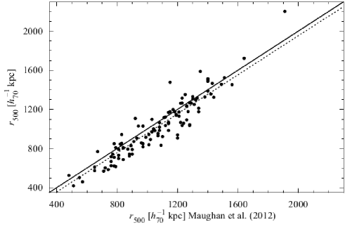
Figure 2: Comparison of the $r_{500}$ values determined by Maughan et al. (2012) and those computed with Eq. 6 to determine $r_{2500}$ and $r_{500}$ in a homogeneous way for our sample.

We computed the total mass using Eq. 5 and assuming a modified $\beta$-model for the gas density profile and an isothermal profile, as in the case for the groups. In Appendix A, we test the assumption of isothermality. By showing this, we are not introducing any systematic error, and we show that the total masses derived in this work are robust. The gas and total masses inside radii $r_{2500}$ and $r_{500}$ are presented in Tab. LABEL:tab:geral. The errors on the total mass determinations are mainly because of the assumption of an isothermal gas.

It is important to state that Piffaretti & Valdarnini (2008) have shown that masses can be underestimated by about 5%, even for the most relaxed clusters. Nagai et al. (2007) found that the gas mass is measured quite accurately ($<\sim 6\%$) in all clusters, while the hydrostatic estimate biases the total mass towards lower values by about 5%-20% throughout the virial region, when compared to the gravitational mass estimates. Thus, we incorporated a 10% error into our $f_{\rm gas}$ error budget for all systems (clusters and groups).

5 Results

We present our results in four different sub-sections. In the first part, we present and discuss the star formation efficiency as a function of total mass computed inside $r_{2500}$ and $r_{500}$ for our sample of 37 systems (nine groups and 28 clusters) with both optical and X-ray available data. In Sect. 5.2, we investigate the difference in mass between the estimated total baryon budget and the WMAP-7 value. Then, we discuss in Sect. 5.3 the gas mass fraction enclosed in $r_{2500}$ and $r_{500}$, and also the differential mass fraction as a function of total mass for our entire sample of 123 systems. Finally, we address the use of clusters, or more precisely, the total baryon budget and the gas mass fraction as a function of redshift, as cosmological tools in Sect.5.4. Given the large scatter observed, we adopt the robust Spearman correlation coefficient $\rho$ and determine the significance of its deviation from zero $P$ (where a small value of $P$ indicates a stronger correlation) to evaluate the significance of the correlations (see Press et al., 1992).

5.1 Cold baryon fraction and star formation efficiency

In this section, we investigate the star formation efficiency and the cold baryon fraction dependences on total mass of the system. The star formation efficiency can be defined as the ratio of stellar to gas mass, and the cold baryon fraction is the ratio between the stellar mass and the total baryon (stars plus ICM) mass. In Fig. 3, we show the star formation efficiency and the cold-baryon fraction as a function of total mass computed for $r_{2500}$ and $r_{500}$.

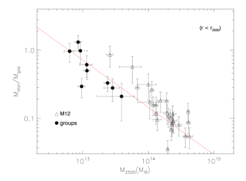
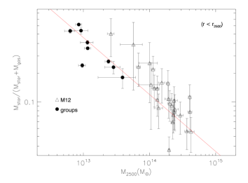
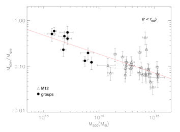
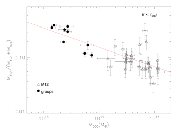
Figure 3: Cold baryon fraction, $M_{\rm star}/(M_{\rm gas}+M_{\rm star}$) and star formation efficiency, $M_{\rm star}/M_{\rm gas}$, as a function of total mass, computed inside $r_{2500}$ (upper panels) and $r_{500}$ (lower panels).

From Fig. 3, we see a clear trend, which suggests that the cold baryon fraction and star formation efficiency decrease with increasing total mass (as reported previously by David et al., 1990; Roussel et al., 2000). We obtained a Spearman correlation coefficient of $\rho=-0.73$ with $P=10^{-7}$ for the correlations within $r_{500}$ and $\rho=-0.84$ with $P=10^{-11}$ for the correlations within $r_{2500}$. In both cases, we had a strong correlation between the cold baryon fraction/star formation efficiency and the total mass.

The star formation efficiency decreases by an order of magnitude for both $r_{2500}$ and $r_{500}$ from groups to massive clusters. From the analysis of twelve groups and clusters, David et al. (1990) also found a strong correlation for $M_{\rm star}/M_{\rm gas}\times M_{\rm tot}$, showing that the $M_{\rm star}/M_{\rm gas}$ ratio varies by more than a factor of five from low to high-mass systems.

5.2 Difference between the observed and WMAP-7 baryon fractions

In Fig. 4, we show the stellar, gas, and total baryon budgets as a function of total mass of the system. We also show the ratio between the total baryon fraction determined by the sum of $f_{\rm star}$ and $f_{\rm gas}$ and the WMAP-7 value as a function of total mass in the bottom panel. The solid lines represent the best linear fits for the total, gas and stellar mass fractions as a function of total mass. We also represent the fits for the stellar mass fraction for groups and clusters separately. As we see, the best fits for the stellar mass fractions differ by more than $3\sigma$ if we separate the 28 clusters from the 9 groups. This suggests that groups and clusters form two distinct populations in terms of stellar content.

The total baryon mass fraction, as shown in Fig. 4, for the mass range analysed here indicates a decrease towards groups and poor-clusters (as mentioned previously). The discrepancy between the total baryon mass fraction and the WMAP-7 value becomes larger with decreasing mass (as already pointed out by some previous works, such as in Gonzalez et al., 2007; Giodini et al., 2009; Andreon, 2010). To use the total baryon fraction of galaxy clusters as a cosmological tool, one thus should consider carefully the sample. These structures range in mass from $M_{500}\sim 10^{13}M_{\odot}$ to $10^{15}M_{\odot}$, and $f_{\rm baryon}$ is not constant for the entire range of mass. We discuss this further in Sect. 6.

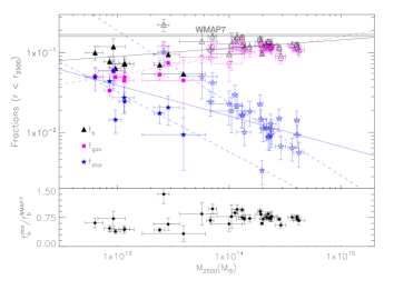
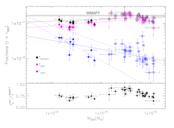
Figure 4: Stellar (blue stars), gas (magenta squares), and total baryon (black triangles) mass fractions as a function of total mass for $r_{2500}$ (top panel) and $r_{500}$ (lower panel). The solid lines correspond to the best linear fit for each relation. The two blue dashed lines correspond to the fits for the groups and clusters separately. On the bottom of each panel, we show the ratio between the total baryon fraction determined by the sum of $f_{\rm star}$ and $f_{\rm gas}$ and the WMAP-7 value as a function of total mass.

5.3 Gas mass fraction within $r_{500}$, and $r_{2500}$, and the differential gas mass fraction ($f_{\rm gas,diff}$)

The gas mass fraction of clusters of galaxies can be used as a cosmological tool, as first done by Allen et al. (2002) and refined later by Allen et al. (2004) and Allen et al. (2008). These studies show an agreement between the gas mass fraction and the $\Lambda$CDM cosmology. Recently, more sophisticated X-ray analyses were done by Ettori et al. (2009) and Mantz et al. (2010). All these studies rely upon the assumption that the gas mass fraction of the cluster sample considered is constant with total mass and redshift.

In this section, we present our results concerning the gas mass fraction dependence on the total mass, making use of our entire sample of 123 objects. We present our results in Fig. 5. We show the strong cool-core clusters in blue (RCC is defined in Maughan et al., 2012, these are the most relaxed clusters in the sample). Cool-core clusters are generally defined by a drop of temperature in the centre which is associated with denser cores that are cooling hydrostatically via bremsstrahlung. They are associated with dynamically relaxed clusters, where the hydrostatic equilibrium equation is valid. However, it seems to be a general agreement between the “true” masses (measured through weak-lensing) and the X-ray derived values inside $r_{\rm 500}$, independent of the dynamical state of the system (Zhang et al., 2010).

In Fig. 5, we show the gas mass fraction inside $r_{2500}$, and $r_{500}$ and the differential gas mass fraction as a function of total mass. The differential gas mass fraction, $f_{\rm gas,diff}$, is defined as the mass fraction within the spherical shell of radii $r_{2500}$ and $r_{500}$; that is, $[M_{\rm gas,500}-M_{\rm gas,2500}]/[M_{\rm tot,500}-M_{\rm tot,2500}]$. We see that there is a $f_{\rm gas}$ dependence on total mass for total masses enclosed in both radii. If we assume a linear dependence (BCES bisector), $f_{\rm gas,2500}-M_{\rm tot,2500}$ ($f_{\rm gas,2500}\propto M_{2500}^{0.17\pm 0.02}$ with a $\rho=0.47$ and $P=2.8\times 10^{-8}$) is compatible with the relation computed for $r_{500}$ within the measurement errors ($f_{\rm gas,500}\propto M_{500}^{0.14\pm 0.02}$ with a $\rho=0.16$ and $P=0.006$). Both relations are steeper than the relation found for the differential gas mass fraction, $f_{\rm gas,diff}\propto M_{\rm tot,500}^{0.02\pm 0.02}$, that is compatible with a flat distribution. We must stress that the trend found here for $f_{\rm gas,500}-M_{\rm tot,500}$ is not as steep as the one presented in Laganá et al. (2011) within 1$\sigma$, which may be because of two major factors: first, we computed the total mass from a scaling relation using the gas mass as a proxy in the previous work, imposing a $f_{\rm gas}$ dependence on $M_{\rm tot}$ and diminishing the scatter in the relation; second, we have assumed an isothermal gas to compute the total mass in the present work, instead of considering the temperature profile. However, the slopes agree within $2\sigma$.

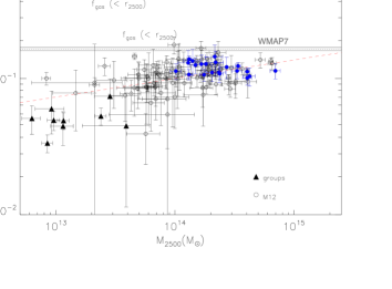
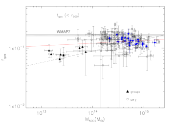
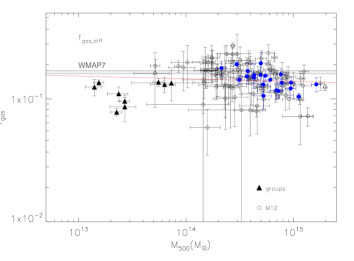
Figure 5: Gas mass fraction as a function of total mass computed within $r_{2500}$ (upper panel), and within $r_{500}$ (middle panel); the differential gas mass fraction, $[M_{\rm gas,500}-M_{\rm gas,2500}]/[M_{\rm tot,500}-M_{\rm tot,2500}]$, as a function of $M_{\rm tot,500}$ (lower panel). The triangles represent the nine groups, while the circles represent the 114 clusters from M12 (we show in blue the strong cool-core clusters). The red lines show the best fits for the entire sample. The dashed line in the middle panel corresponds to the best fit found by Laganá et al. (2011).

The differential gas mass fraction shown in Fig. 5 is higher than the cumulative measures, reaching the universal baryon fraction for systems with mass $M_{500}\sim 10^{14}M_{\odot}$. Clearly, the differential gas mass fraction is constant at the 1$\sigma$ level and provides a better constraint for cosmology, although the statistical scatter is very large. For groups (i.e., the systems in our sample with $M_{500}<10^{14}M_{\odot}$), we still observe lower values for the differential gas mass fraction when compared to the WMAP-7 result. Since our sample includes few systems in this mass regime, we cannot derive firm conclusions.

Comparing the three plots in Fig. 5, we conclude that the observed $f_{\rm gas}-M_{\rm tot}$ trend found for groups and clusters is due to the lack of gas enclosed inside $r_{2500}$ for groups and poor clusters, as proposed by Sun (2012), owing to non-thermal processes, such as supernova feedback, that are more efficient in low mass systems because of the shallower potential well. From their hydrodynamical simulations, Young et al. (2011) reported that the injection of entropy has removed gas from the cores of the low-mass systems and pushed the gas out to larger radii between $r_{500}$ and $r_{200}$.

When we analyse the differential stellar mass fractions (i.e., $f_{\rm star}$ in the annulus between $r_{2500}$ and $r_{500}$ for the 37 systems for which we have SDSS data) we also do not observe any trend as a function of $M_{500}$.

5.4 Cosmological constraints from the total baryon budget and from the $f_{\rm gas}$ vs. redshift relation

As mentioned before, the X-ray data analysis of galaxy clusters can provide reliable constraints on cosmology from the total baryon budget and the gas mass fraction dependence on the redshift. One of the classical methods to infer $\Omega_{\rm m}$ assumes that the baryon-to-total mass ratio should closely match the cosmological values, and thus $\Omega_{\rm b}/\Omega_{\rm m}\sim M_{\rm b}/M_{\rm tot}$ (White et al., 1993; Evrard, 1997). Combining $\Omega_{\rm b}=0.0456$ (Jarosik et al., 2011) with our values for the baryon fraction obtained in Sect. 5.1, our results imply $\Omega_{m}<0.55$ (assuming the lowest $f_{\rm b}$ value and agreeing with Ettori & Fabian, 1999), and if we take the highest significant estimates for $f_{\rm b}$, $\Omega_{m}>0.22$.

In addition to the calculation of $\Omega_{m}$ based on the total baryon budget, the gas mass fraction has been used to obtain more rigorous constraints on cosmology that probes the acceleration of the universe. The apparent behaviour of $f_{\rm gas}$ with redshift can constrain the cosmic acceleration, as studied in Ettori & Fabian (1999) and Allen et al. (2004, 2008). This constraint originates because $f_{\rm gas}$ measurements depends on the distance to the cluster ($f_{\rm gas}\propto d^{1.5}$).

The gas mass fraction for the present sample was computed, assuming the default $\Lambda$CDM cosmology, and we show the gas mass fraction determined inside $r_{2500}$ ($f_{\rm gas,2500}$) and $r_{500}$ ($f_{\rm gas,500}$) as a function of redshift in Fig. 6. On the bottom of each panel, we show the mean gas mass fraction value computed for bins of 0.2 in redshift as a function of the mean redshift with red points, and the errors are the standard errors on the mean.

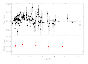
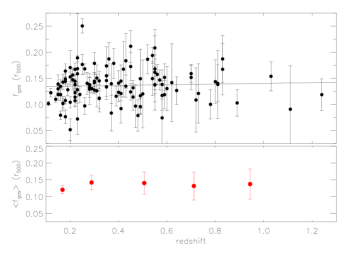
Figure 6: Gas fraction as a function of redshift for $r_{2500}$ (upper panel) and $r_{500}$ (lower panel). The black lines represent the best linear fit for the data.

From this figure, we can see that the gas mass fraction values determined for $r_{2500}$ and $r_{500}$ show little variation with redshift. Assuming $f_{\rm gas(z)}=A+B\times z$, we obtained $A=0.130\pm 0.009$ and $B=0.010\pm 0.015$ for $r_{500}$, and determined $A=0.110\pm 0.008$ and $B=-0.019\pm 0.013$ for $r_{2500}$. From these results, we verified that the enclosed gas mass fraction does not depend on redshift at a $2\sigma$ level in both cases.

From our analysis, we cannot attribute the slight decrease of $f_{\rm gas,2500}$ with redshift to evolution of $f_{\rm gas}$. Selection biases may have led to the enhanced mean gas mass fraction at around z=0.3 and may have driven the observed trend, as recently reported by Landry et al. (2012).

6 Discussion

In this section, we further discuss the results obtained in this work and compare them to previous observational and theoretical ones.

6.1 Stellar and gas mass dependence on total mass

The trends shown in Fig. 3 can be explained by a decrease in the stellar mass with an increase in cluster mass. Alternatively, the gas mass can increase for more massive systems. From previous results in the literature (David et al., 1990; Lin et al., 2003; Laganá et al., 2008; Giodini et al., 2009; Laganá et al., 2011; Zhang et al., 2011), we observe both behaviours, but the decrease in stellar mass fraction as a function of total mass is more significant than the gas mass increase in the same range. This provides evidence that there is no well-tuned balance between the gas and stellar mass fractions. This evidence suggests that the variation in star formation efficiency is because of the variation in stellar mass, which arises from the decrease in efficiency of tidal interactions among galaxies, the removal of the gas reservoir of galaxies due to the motion of galaxies through the ICM, or feedback processes that may quench star-formation. Recent numerical simulation results from Dubois et al. (2013) supported this scenario. According to their results, AGN feedback alone is able to significantly alter the stellar mass content by quenching star formation.

During mergers to form rich clusters, the gas within the system will be shocked and heated to the virial temperature. As mergers progress, more massive systems are formed, and the gas is progressively heated to higher temperatures. Thus, cooling and galaxy formation are inhibited. Since rich clusters are formed from many mergers, this explains why this large gas fraction of the gas is not consumed to form stars. In contrast, less massive systems, such as groups, have experienced fewer mergers. Therefore their gas is cooler and more stars are formed within the galaxies. As a consequence, the star formation efficiency is higher in groups, which indicates that physical mechanisms that depend on the virial mass, such as ram-pressure stripping, are driving galaxy evolution within clusters and groups. This result is important to provide constraints on the role of thermodynamical processes for groups and clusters and seems to agree with theoretical expectations from hydrodynamical simulations by Springel & Hernquist (2003). In their models, the integrated star formation efficiency as a function of halo mass, which varies from $10^{8}$ to $10^{15}M_{\odot}$, falls by a factor of five to ten over the cluster mass scale, due to the less efficient formation of cooling flows for more massive haloes (in their case, with temperature above $10^{7}$ K, what comprises the entire range of mass analysed in this work).

Recently, Planelles et al. (2013) carried out two sets of simulations including radiative cooling, star formation and feedback from supernovae and in one of which they also accounted for the effect of feedback from AGN. These authors found that both radiative simulation sets predict a trend of stellar mass fraction with cluster mass that tends to be weaker than the observed one. However this tension depends on the particular set of observational data considered. Including the effect of AGN feedback alleviates this tension on the stellar mass and predicts values of the hot gas mass fraction and total baryon fraction to be in closer agreement with observational results. Also, Zehavi et al. (2012) studied the evolution of stellar mass in galaxies as a function of host halo mass using semi-analytic models, and their results agree with our findings of a varying star formation efficiency. These latter authors found that baryon conversion efficiency into stars has a peaked distribution with halo mass and that the peak location shifts toward lower mass from z$\sim$ 1 to z$\sim$ 0. Another difference between low- and high-mass haloes is that the stellar mass in low-mass haloes grows mostly by star formation since z$\sim$1. In contrast, most of the stellar mass is assembled by mergers in high-mass haloes.

6.2 The ICL contribution to the total baryon budget

To account for the difference in baryons at the low-mass end (see Fig. 4), where the total baryon budget is still significantly below the value of WMAP-7, there are two possibilities. The first possibility is that the discrepancy in baryon mass fraction is because of feedback mechanisms, as expected by many studies (including Bregman, 2007; Giodini et al., 2009). Recent numerical simulations performed by Dai et al. (2010) proposed that the baryon loss mechanism is primarily controlled by the depth of the potential well: the baryon loss is not significant for deep potential wells (rich clusters), while for lower-mass clusters and groups the baryon loss becomes increasingly important. Baryons can be expelled from the central regions beyond $r_{500}$. The second possibility is to account for baryons in other forms: for example, the increase in the stellar light via intra-cluster light (ICL) which increases the stellar mass.

ICL is one of the most important sources of unaccounted baryons, and observational results have shown that it may represent from 10% to 40% of the total cluster light (e.g., Feldmeier et al., 2002; Zibetti et al., 2005; Krick & Bernstein, 2007; Gonzalez et al., 2007). However, recently, Burke et al. (2012) found that the ICL constitutes only 1-4% of the total cluster light within $r_{\rm 500}$ in high-z clusters.

To investigate the ICL contribution as a function of system total mass, we computed the difference between the observed total baryon budget and the WMAP-7 value, which is taken to be: $M_{\rm diff}=(f_{b}^{WMAP-7}-f_{b}^{obs})\times M_{500},$ where $f_{b}^{WMAP-7}$ is the WMAP-7 value; $f_{b}^{obs}$ is the observed baryon mass fraction that we computed for our systems; and $M_{500}$ is the total mass computed in the $r_{500}$ radius. We then assumed that this difference in mass is under the form of luminous matter. To compute the corresponding “missing stellar surface brightness”, we assumed a mass-to-light ratio for ellipticals of $M/L=1.7\leavevmode\nobreak\ M_{\odot}/L_{\odot}$ (Kauffmann et al., 2003) to convert the difference in mass into a difference in luminosity. We then convert the luminosity in surface brightness by dividing the area inside of $r_{500}$.

In Fig. 7, we show the missing stellar mass divided by the total stellar mass as a function of total mass (upper panel), the missing stellar surface brightness as a function of total mass (middle panel), and the ratio between the stellar surface brightness and the BCG magnitude as a function of total mass. Since the stellar mass fraction decreases for massive clusters (Fig. 4) one could conclude that the ICL could be more important in clusters of galaxies because the measured stellar light fraction of the ICL has not been considered. As a direct consequence of the stellar mass dependence on total mass, we observe an increase of the missing-to-total stellar mass ratio as a function of the total mass of the system, as shown in the upper panel of Fig. 7. In this panel, groups and clusters seem to be two distinguished populations, which are comparable to the behaviour observed in Fig. 4. Then, if we think in terms of missing surface brightness, groups seems to present fainter values than clusters. This means that it would be easier to detect the ICL contribution is clusters than in groups.

However, from the values obtained here, the stellar component would have to increase by a factor of three to be able to explain the baryon deficit with intra-cluster light for low-mass systems. Moreover, such a high amount of ICL would be visible in current observations. Although a large sample of clusters and groups is needed for further constraints on the photometrical properties and for the ICL formation mechanism, it is very unlikely that the ICL will be able to answer the baryon deficit problem.

Figure 7: Top: “missing stellar mass” to total stellar mass ratio as a function of $M_{2500}$ (left panel) and $M_{500}$ (right panel); Middle: “missing stellar surface brightness” as a function of total mass for $r_{2500}$ (left panel) and $r_{500}$ (right panel); Botton: “missing stellar surface brightness” to BCG magnitude ratio as a function of $M_{2500}$ (left panel) and $M_{500}$ (right panel).

Even by considering the uncertainties associated with our total baryon fraction and the WMAP-7 measurement, the two values are discrepant at the $5\sigma$ level for systems with mass $M_{500}<10^{14}M_{\odot}$. It is therefore probable that either the baryon mass fraction within $r_{500}$ in groups is different from the universal value, or that there are still unaccounted baryons (other than ICL) in the low-mass regime.

7 Conclusions

We have investigated the baryon content of a sample of 123 galaxy clusters and groups, whose mass spans a broad range (from groups of $M_{500}\sim 10^{13}M_{\odot}$ up to clusters of $M_{500}=4\times 10^{15}M_{\odot}$). We measured the cluster gas and total masses from X-ray data analysis, and we computed the stellar masses for 37 out of 123 galaxy clusters and groups using DR8-SDSS data. We summarise our results and discussions in the following points:

• For a subsample of 37 systems for which we had both optical and X-ray data we derived quantities inside $r_{2500}$ and $r_{500}$ to investigate the stellar, gas and total mass fractions dependence on total mass. We confirmed the previous trend found in the literature: the star formation efficiency is lower for more massive clusters. It decreases by an order of magnitude from groups to clusters inside both $r_{2500}$ and $r_{500}$. We observe a decrease of the cold baryon fraction and of the star formation efficiency from $r_{2500}$ to $r_{500}$.

• Star-formation efficiency is lower in galaxy clusters than in groups, which suggests that the gas reservoir of the galaxies during cluster formation in more massive clusters are more affected by mechanisms, such as ram-pressure, that quench the star formation. Physical mechanisms depending on the total mass of the system may be driving galaxy evolution in groups and clusters. This observational result agrees with hydrodynamical simulations.

• For the entire sample of 123 systems, we analysed the gas mass fraction inside $r_{2500}$, and $r_{500}$ and also the differential gas mass fraction ($f_{\rm gas,2500}$ - $f_{\rm gas,500}$) dependence on total mass. We found that the gas fraction depends on the total mass inside both radii, with the dependence being steeper for the inner radius. However, we found that for systems more massive than $M_{\rm tot}>10^{14}M_{\odot}$, the differential gas mass fraction shows no dependence on total mass, which provides evidence that groups cannot retain gas in the inner parts in the same way clusters do. Since groups have shallower potential wells, non-thermal processes are more important than in clusters, and AGN feedback, for instance, could expel the gas towards the outer radii of groups. This result is an indication that such processes must play a more important role in the centres of low-mass systems than in massive clusters.

• The differential gas mass fraction is higher than the cumulative measures and clearly more constant as a function of total mass, which provides better constraints for cosmology.

• Our results show that non-thermal processes play different but important roles on galaxy evolution in groups and clusters. While in groups, the gas is more affected because of the lower potential well, in galaxy clusters, the cold baryons (stars in galaxies) are more affected due to ram-pressure stripping. These mechanisms make the baryon distribution in these two structures different. Many studies have indeed reported systematic differences between the physical properties of groups and the clusters.

• To investigate the contribution of the ICL to the baryon budget, we computed the difference in mass between the WMAP-7 value and the observed baryon fraction in terms of surface brightness. The values found here for the expected missing surface brightness for clusters of galaxies are similar to the ICL surface brightness detected in the literature, which span the range of $\sim 24<\mu_{\rm r}<28$. If the difference between the observed baryon fraction and the WMAP-7 value is because of luminous matter that is spread throughout the volume of the system, as a direct consequence of $M_{\rm star}$ dependence on $M_{\rm tot}$, we observe a small increase in Missing Mass/$M_{\rm star}$ with total mass, and groups and clusters seem to be separated into two distinct populations. However, we have a high scatter inside both $r_{2500}$ and $r_{500}$. In terms of missing surface brightness, we observe a small decrease as a function of total mass also for the ratio between the missing surface brightness and the BCG magnitude inside $r_{500}$, but it is difficult to spot a clear trend from these panels.

• Combining the baryon-to-total mass fraction with primordial nucleosynthesis measurements, our results indicate that $0.17<\Omega_{\rm m}<0.55$. We also observed that the gas mass fraction that is enclosed within $r_{2500}$ and $r_{500}$ does not depend on redshift at the 2-sigma level, which is very important in the use of clusters of galaxies as a cosmological tool to constrain the cosmic acceleration.

Appendix A Testing the isothermal assumption to compute $r_{500}$ and $M_{\rm tot,500}$

To test if the assumption of an isothermal cluster would introduce any systematic effect on the total mass determination, biasing low the total mass of cool-core clusters, we consider eight cool-core clusters from Vikhlinin et al. (2006) for which all the necessary parameters were available. We computed $r_{500}$, $M_{\rm tot,500}$ and $M_{\rm gas,500}$ by considering their Eq. (6) to describe the temperature profile and a mean temperature, $T_{\rm mg}$, in the isothermal case. For both cases, the emission measure profile is given by the sum of a modified $\beta$-model profile and a second $\beta$-model component with a small core radius, as stated in their Eq. (2).

In Fig. A.1, we show the comparison between $r_{500}$, $M_{\rm tot,500}$ and $M_{\rm gas,500}$ which is computed in both ways, using a temperature profile and assuming an isothermal case. To compute the gas mass, we do not use the temperature profile, since the values of $r_{500}$ change. The enclosed $M_{\rm gas,500}$ will also change, and for completeness we thus, show the comparison for the gas masses computed in both ways in Fig. A.1.

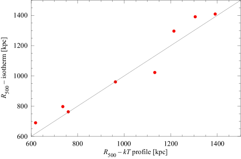
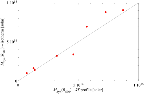
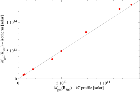
Figure 8: Upper panel: $r_{500}$ computed assuming an isothermal gas, as a function of $r_{500}$ computed, assuming the temperature profile given in Vikhlinin et al. (2006). Middle panel: $M_{\rm tot,500}$ computed, assuming an isothermal gas, as a function of $M_{\rm tot,500}$ computed, assuming the temperature profile given in Vikhlinin et al. (2006). Lower panel:$M_{\rm gas,500}$ computed, assuming an isothermal gas as a function of $M_{\rm gas,500}$ computed, assuming the temperature profile given in Vikhlinin et al. (2006).

As we can see from Fig. A.1, the assumption of isothermality does not introduce any systematic error in either the total mass or $r_{500}$. Moreover, the values are in good agreement, which is shown even for cool-core clusters, that the derived values in this work are robust.

Appendix B Geometric correction

The stellar mass is measured in a cone, along the line-of-sight of radius $r_{2500}$ or $r_{500}$ at the group/cluster distance. For simplicity, we will approximate the cone by a cylinder, since the distance of the cluster is much larger than its radius. The length of the cylinder can only be roughly estimated by the given scatter in redshift space, when enough galaxies have a redshift determination. On the other hand, the gas and dynamical masses are measured in spheres of radius $r_{2500}$ or $r_{500}$. Compared to the sphere, the cylinder will cover a greater volume in space and therefore, a geometric correction is needed.

To estimate this correction, one must assume (or determine) the spatial distribution of galaxies in clusters and groups. Using SDSS data, Hansen et al. (2005) showed that the radial profile of the galaxy distribution is well represented by a NFW profile (Navarro et al., 1997), which is shallower than the dark matter distribution in clusters with a concentration parameter $c\approx 2$–4.

Given a radial profile, the mass excess,$\Upsilon$, of a cylinder compared to a sphere is:

$$\Upsilon=M_{\rm cyl}/M_{\rm sph}\,,$$ (10)

where

$$M_{\rm sph}=4\pi\int_{0}^{R_{\rm max}}\rho(r)r^{2}dr\quad\mbox{and}\quad$$ (11)

$$M_{\rm cyl}=4\pi\int_{0}^{z_{\rm max}}\!\int_{0}^{R_{\rm max}}\rho(R,z)RdR\,dz\,.$$ (12)

Here, $R_{\rm max}$ is the sphere radius of either $r_{500}$ or $r_{2500}$, and $z_{max}$ is half the length of the cylinder (i.e., we are measuring the mass between $\pm z_{\rm max}$). Although cumbersome, $\Upsilon$ can be determined analytically, if we assume a NFW profile. In terms of the concentration parameter, $c\equiv r_{200}/r_{s}$, we have:

$$\begin{split}\Upsilon=&\sqrt{a^{2}c^{2}-1}\times[(1+ac)\ln(1+ac)-ac]\times(1+ac)^{-1}\times\\ &\bigg{[}\arctan\left(\frac{bc}{\sqrt{a^{2}c^{2}-1}}\right)-\arctan\left(\frac{b}{\sqrt{(a^{2}+b^{2})(a^{2}c^{2}-1)}}\right)+\\ &\sqrt{a^{2}c^{2}-1}\times\ln{\left(\frac{a+abc}{b+\sqrt{a^{2}+b^{2}}}\right)}\bigg{]}^{-1}\,,\end{split}$$ (13)

where $a=R_{\rm max}/r_{200}$ and $b=z_{\rm max}/r_{200}$.

For a NFW profile, $r_{500}/r_{200}=0.61$–0.65 for $c=2$–4 and $r_{2500}/r_{200}=0.22$–0.28 also for $c=2$–4. The mass excess in the cylinder is shown in Fig. B.1.:

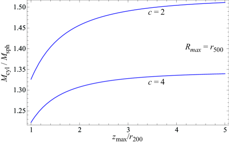
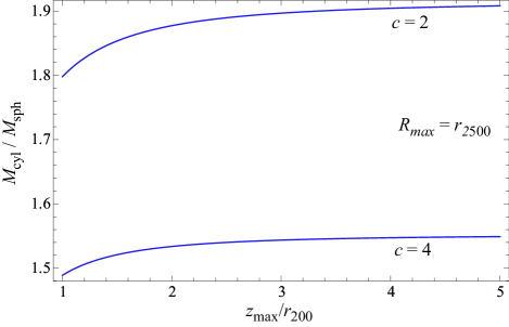
Figure 9: Upper panel: for a fixed $R_{\rm max}=r_{500}$, mass excess as a function of $z_{\rm max}/r_{200}$, for two NFW concentration parameters $c$. Lower panel: same as upper panel but for $R_{\rm max}=r_{2500}$.

If we assume that we are including galaxies up to $\sim 3r_{200}$, then we very roughly have the following mass excesses: $\Upsilon\sim 1.4$ for spheres of $r_{500}$, and $\Upsilon\sim 1.7$ for spheres of $r_{2500}$. To compare the stellar mass in galaxies with the gas and dynamical masses, the former should therefore be divided by the above $\Upsilon$, depending on the extraction radius.

Table 2: General properties, X-ray parameters and stellar masses derived for our sample

Groups
Name	z	RA	Dec	$r_{2500}$	$r_{500}$	$<kT>$	$M_{\rm gas,2500}$	$M_{\rm gas,500}$	$M_{\rm tot,2500}$	$M_{\rm tot,500}$	$M_{\rm star,2500}$	$M_{\rm star,500}$
				($h_{70}^{-1}$) kpc	($h_{70}^{-1}$) kpc	(keV)	$(10^{12}M_{\odot})$	$(10^{12}M_{\odot})$	$(10^{13}M_{\odot})$	$(10^{13}M_{\odot})$	$(10^{12}M_{\odot})$	$(10^{12}M_{\odot})$
NGC1132	0.023	02h52m51.9s	–01d16m29s	171.5	383.5	0.98 $\pm$ 0.10	0.29 $\pm$ 0.03	1.24 $\pm$ 0.03	0.85 $\pm$ 0.09	1.55 $\pm$ 0.17	0.37$\pm$ 0.09	0.60 $\pm$ 0.12
RBS461	0.030	03h41m21.7s	+15d24m18s	262.4	586.8	2.14 $\pm$ 0.46	0.55 $\pm$ 0.09	2.09 $\pm$ 0.39	0.92 $\pm$ 0.25	2.70 $\pm$ 0.73	0.54 $\pm$ 0.15	0.95 $\pm$ 0.25
NGC4104	0.028	12h06m39.0s	+28d10m27s	224.7	502.5	1.63 $\pm$ 0.18	0.57 $\pm$ 0.05	2.05 $\pm$ 0.09	1.16 $\pm$ 0.13	2.70 $\pm$ 0.48	0.28 $\pm$ 0.07	0.69 $\pm$0.18
NGC4325	0.026	12h23m06.7s	+10d37m16s	182.1	408.6	0.89 $\pm$ 0.11	0.47 $\pm$ 0.05	1.50 $\pm$ 0.02	0.96 $\pm$ 0.12	2.27 $\pm$ 0.27	0.14 $\pm$ 0.04	0.29 $\pm$ 0.08
NGC5098	0.037	13h20m16.2s	+33d08m39s	154.1	344.6	0.94 $\pm$ 0.17	0.32 $\pm$ 0.05	1.30 $\pm$ 0.21	0.63 $\pm$ 0.11	1.41 $\pm$ 0.25	0.31 $\pm$ 0.08	0.55 $\pm$ 0.14
Abell1991	0.059	14h54m30.2s	+18d37m51s	251.9	563.3	2.20 $\pm$ 0.57	2.11 $\pm$ 0.46	6.68 $\pm$ 0.12	2.85 $\pm$ 0.74	6.33 $\pm$ 1.66	0.59 $\pm$ 0.18	1.09 $\pm$ 0.30
AWM4	0.032	16h04m57.0s	+23d55m14s	245.0	547.8	2.40 $\pm$ 0.26	1.27 $\pm$ 0.12	5.60 $\pm$ 0.29	2.39 $\pm$ 0.26	5.55 $\pm$ 0.61	0.42 $\pm$ 0.10	0.62 $\pm$ 0.14
IC1262	0.033	17h33m02.0s	+43d45m35s	284.8	636.9	2.64 $\pm$ 1.51	1.75 $\pm$ 0.64	6.36 $\pm$ 0.65	3.90 $\pm$ 1.23	7.32 $\pm$ 4.20	0.37 $\pm$ 0.11	0.65 $\pm$ 0.18
RXCJ2315.7-0222	0.027	23h15m44.1s	–02d22m59s	191.0	427.1	1.39 $\pm$ 0.23	0.51 $\pm$ 0.06	1.86 $\pm$ 0.19	1.15 $\pm$ 0.25	2.37 $\pm$ 0.51	0.31 $\pm$ 0.09	0.70 $\pm$ 0.20
Clusters from M12
Name	z	RA	Dec	$r_{2500}$	$r_{500}$	$<kT>$	$M_{\rm gas,2500}$	$M_{\rm gas,500}$	$M_{\rm tot,2500}$	$M_{\rm tot,500}$	$M_{\rm star,2500}$	$M_{\rm star,500}$
				($h_{70}^{-1}$) kpc	($h_{70}^{-1}$) kpc	(keV)	$(10^{13}M_{\odot})$	$(10^{13}M_{\odot})$	$(10^{14}M_{\odot})$	$(10^{14}M_{\odot})$	$(10^{13}M_{\odot})$	$(10^{13}M_{\odot})$
MS0015.9+1609	0.54	00h18m33.631s	+16d26m13.56s	445.6	1092.6	8.3 $\pm$0.5	3.34 $\pm$ 0.17	12.9 $\pm$0.6	2.26$\pm$0.14	6.67 $\pm$0.40	-	-
RXJ0027.6+2616	0.37	00h27m46.051s	+26d16m19.92s	328.4	914.8	4.8 $\pm$1.0	0.78 $\pm$ 0.14	4.5 $\pm$0.8	0.74$\pm$0.15	3.19 $\pm$0.66	-	-
CLJ0030+2618	0.50	00h30m33.948s	+26d18m08.28s	291.2	811.4	4.1 $\pm$1.7	0.60 $\pm$ 0.21	3.1 $\pm$1.1	0.60$\pm$0.25	2.60 $\pm$1.08	-	-
MS0015.9+1609	0.54	00h18m33.631s	+16d26m13.56s	445.6	1092.6	8.3 $\pm$0.5	3.34 $\pm$ 0.17	12.9 $\pm$0.6	2.26$\pm$0.14	6.67 $\pm$0.40	-	-
RXJ0027.6+2616	0.37	00h27m46.051s	+26d16m19.92s	328.4	914.8	4.8 $\pm$1.0	0.78 $\pm$ 0.14	4.5 $\pm$0.8	0.74$\pm$0.15	3.19 $\pm$0.66	-	-
CLJ0030+2618	0.50	00h30m33.948s	+26d18m08.28s	291.2	811.4	4.1 $\pm$1.7	0.60 $\pm$ 0.21	3.1 $\pm$1.1	0.60$\pm$0.25	2.60 $\pm$1.08	-	-
A68	0.26	00h37m06.089s	+09d09m33.04s	559.6	1352.7	7.8 $\pm$1.0	2.98 $\pm$ 0.32	8.8 $\pm$0.9	3.22$\pm$0.41	9.10 $\pm$1.17	-	-
A115	0.20	00h55m50.688s	+26d24m37.80s	429.4	1035.7	6.7 $\pm$1.0	1.45 $\pm$ 0.18	6.5 $\pm$0.8	1.37$\pm$0.20	3.84 $\pm$0.57	0.14 $\pm$ 0.04	0.81$\pm$ 0.24
A209	0.21	01h31m53.520s	–13d36m46.44s	479.9	1213.1	7.4 $\pm$0.5	2.23 $\pm$ 0.13	9.7 $\pm$0.5	1.93$\pm$0.13	6.22 $\pm$0.42	-	-
CLJ0152.7-1357S	0.83	01h52m39.888s	–13d58m26.76s	239.7	625.3	4.9 $\pm$1.1	0.50 $\pm$ 0.09	3.0 $\pm$0.6	0.50$\pm$0.11	1.77 $\pm$0.40	-	-
A267	0.23	01h52m42.144s	+01d00m41.29s	404.3	953.3	4.4 $\pm$0.5	1.61 $\pm$ 0.15	5.2 $\pm$0.5	1.18$\pm$0.13	3.10 $\pm$0.35	0.25 $\pm$ 0.07	0.55 $\pm$ 0.16
CLJ0152.7-1357N	0.83	01h52m44.280s	–13d57m19.08s	239.0	621.1	4.9 $\pm$0.9	0.53 $\pm$ 0.08	3.2 $\pm$0.5	0.49$\pm$0.09	1.73 $\pm$0.32	-	-
MACSJ0159.8-0849	0.41	01h59m49.368s	–08d50m00.42s	570.7	1296.3	10.2 $\pm$0.9	4.09 $\pm$ 0.30	11.5 $\pm$0.8	4.05$\pm$0.36	9.49 $\pm$0.84	-	-
CLJ0216-1747	0.58	02h16m32.856s	–17d47m32.28s	318.9	849.9	5.6 $\pm$3.8	0.47 $\pm$ 0.27	2.4 $\pm$1.4	0.87$\pm$0.59	3.28 $\pm$2.22	-	-
RXJ0232.2-4420	0.28	02h32m18.216s	–44d20m49.56s	539.0	1317.5	8.0 $\pm$1.4	3.58 $\pm$ 0.52	11.2 $\pm$1.6	2.97$\pm$0.52	8.68 $\pm$1.52	-	-
MACSJ0242.5-2132	0.31	02h42m35.856s	–21d32m26.16s	439.9	985.5	5.5 $\pm$0.7	2.14 $\pm$ 0.23	5.7 $\pm$0.6	1.67$\pm$0.21	3.76 $\pm$0.48	-	-
A383	0.19	02h48m03.432s	–03d31m45.87s	425.1	971.2	4.5 $\pm$0.3	1.40 $\pm$ 0.08	4.0 $\pm$0.2	1.31$\pm$0.09	3.13 $\pm$0.21	0.22 $\pm$ 0.07	0.49 $\pm$ 0.15
MACSJ0257.6-2209	0.32	02h57m41.328s	–22d09m14.40s	455.5	1199.4	6.7 $\pm$0.9	1.99 $\pm$ 0.22	7.6 $\pm$0.9	1.87$\pm$0.25	6.83 $\pm$0.92	-	-
MS0302.7+1658	0.42	03h05m31.656s	+17d10m10.56s	308.9	697.8	3.3 $\pm$0.8	0.82 $\pm$ 0.17	2.5 $\pm$0.5	0.66$\pm$0.16	1.51 $\pm$0.37	-	-
CLJ0318-0302	0.37	03h18m33.456s	–03d02m57.30s	435.4	1030.8	5.4 $\pm$1.7	1.31 $\pm$ 0.34	3.8 $\pm$1.0	1.73$\pm$0.54	4.58 $\pm$1.44	-	-
MACSJ0329.6-0211	0.45	03h29m41.520s	–02d11m45.99s	349.9	839.6	4.5 $\pm$0.5	1.74 $\pm$ 0.16	5.7 $\pm$0.5	0.98$\pm$0.11	2.72 $\pm$0.30	-	-
MACSJ0404.6+1109	0.36	04h04m32.664s	+11d08m16.80s	343.1	834.5	5.5 $\pm$0.7	0.84 $\pm$ 0.09	4.5 $\pm$0.5	0.83$\pm$0.11	2.39 $\pm$0.30	-	-
MACSJ0429.6-0253	0.40	04h29m35.952s	–02d53m06.21s	456.1	1065.8	6.5 $\pm$0.7	2.27 $\pm$ 0.20	6.5 $\pm$0.6	2.05$\pm$0.22	5.24 $\pm$0.56	-	-
RXJ0439.0+0715	0.23	04h39m00.672s	+07d16m03.75s	440.1	1169.6	5.3 $\pm$0.4	2.05 $\pm$ 0.13	7.3 $\pm$0.5	1.52$\pm$0.12	5.72 $\pm$0.43	-	-
RXJ0439+0520	0.21	04h39m02.304s	+05d20m43.26s	387.7	848.8	3.9 $\pm$0.4	1.15 $\pm$ 0.10	3.1 $\pm$0.3	1.02$\pm$0.10	2.14 $\pm$0.22	-	-
MACSJ0451.9+0006	0.43	04h51m54.408s	+00d06m19.13s	363.0	892.7	5.0 $\pm$1.1	1.50 $\pm$ 0.27	5.9 $\pm$1.1	1.07$\pm$0.24	3.19 $\pm$0.70	-	-
A521	0.55	04h54m11.184s	–03d00m53.85s	292.4	906.2	4.8 $\pm$0.2	0.67 $\pm$ 0.02	6.8 $\pm$0.2	0.46$\pm$0.02	2.73 $\pm$0.11	-	-
A520	0.25	04h54m06.576s	–10d13m15.24s	447.1	1251.2	6.5 $\pm$0.3	2.02 $\pm$ 0.08	10.3 $\pm$0.4	1.55$\pm$0.07	6.78 $\pm$0.31	-	-
MS0451.6-0305	0.20	04h54m09.600s	+02d55m28.63s	447.1	1148.9	7.6 $\pm$1.2	3.60 $\pm$ 0.47	12.6 $\pm$1.7	2.31$\pm$0.36	7.83 $\pm$1.24	-	-
CLJ0522-3625	0.47	05h22m14.832s	–36d24m57.60s	318.7	845.2	4.3 $\pm$1.4	0.60 $\pm$ 0.16	2.8 $\pm$0.7	0.76$\pm$0.25	2.84 $\pm$0.93	-	-
CLJ0542.8-4100	0.64	05h42m50.208s	–41d00m04.32s	346.4	872.4	6.2 $\pm$1.0	1.11 $\pm$ 0.15	4.8 $\pm$0.7	1.20$\pm$0.19	3.83 $\pm$0.62	-	-
MACSJ0647.7+7015	0.58	06h47m50.160s	+70d14m55.68s	533.6	1231.0	11.3 $\pm$2.1	3.88 $\pm$ 0.60	11.8 $\pm$1.8	4.09$\pm$0.76	10.04$\pm$1.86	-	-
1E0657-56	0.30	06h58m30.000s	–55d56m39.12s	692.9	1722.6	11.7 $\pm$0.5	8.57 $\pm$ 0.31	25.0 $\pm$0.9	6.40$\pm$0.27	19.66$\pm$0.84	-	-
MACSJ0717.5+3745	0.55	07h17m31.680s	+37d45m31.68s	400.9	1513.0	10.6 $\pm$1.0	2.77 $\pm$ 0.22	24.4 $\pm$1.9	1.66$\pm$0.16	17.81$\pm$1.68	-	-
A586	0.17	07h32m20.160s	+31d37m55.92s	557.8	1265.8	7.6 $\pm$0.8	2.45 $\pm$ 0.22	6.9 $\pm$0.6	2.91$\pm$0.31	6.81 $\pm$0.72	0.2 $\pm$ 0.06	2.97 $\pm$ 0.89
MACSJ0744.9+3927	0.70	07h44m52.320s	+39d27m26.64s	392.2	1017.6	8.1 $\pm$0.7	2.60 $\pm$ 0.19	10.3 $\pm$0.7	1.86$\pm$0.16	6.49 $\pm$0.56	-	-
A665	0.18	08h30m57.360s	+65d50m33.36s	481.6	1357.3	7.8 $\pm$0.4	2.39 $\pm$ 0.10	12.6 $\pm$0.5	1.90$\pm$0.10	8.50 $\pm$0.44	0.43 $\pm$ 0.13	0.58 $\pm$ 0.17
A697	0.28	08h42m57.600s	+36d21m55.80s	578.7	1455.7	10.2 $\pm$0.8	4.34 $\pm$ 0.28	16.1 $\pm$1.1	3.67$\pm$0.29	11.68$\pm$0.92	0.34 $\pm$ 0.11	0.70 $\pm$ 0.21
CLJ0848.7+4456	0.57	08h48m47.760s	+44d56m13.92s	199.7	460.7	2.0 $\pm$0.2	0.19 $\pm$ 0.02	0.8 $\pm$0.1	0.21$\pm$0.02	0.52 $\pm$0.05	-	-
ZWCLJ1953	0.32	08h50m06.960s	+36d04m17.40s	441.9	1057.0	6.1 $\pm$0.6	1.96 $\pm$ 0.16	6.8 $\pm$0.6	1.71$\pm$0.17	4.67 $\pm$0.46	-	-
CLJ0853+5759	0.48	08h53m14.880s	+57d59m57.48s	298.5	943.1	5.1 $\pm$1.5	0.42 $\pm$ 0.10	3.1 $\pm$0.8	0.63$\pm$0.18	3.97 $\pm$1.17	-	-
MS0906.5+1110	0.18	09h09m12.720s	+10d58m32.88s	405.7	923.0	4.7 $\pm$0.3	1.28 $\pm$ 0.07	4.4 $\pm$0.2	1.13$\pm$0.07	2.67 $\pm$0.17	0.28 $\pm$0.09	0.92 $\pm$0.31
RXJ0910+5422	1.11	09h10m44.880s	+54d22m07.68s	161.6	524.9	2.7 $\pm$1.9	0.20 $\pm$ 0.12	1.3 $\pm$0.8	0.21$\pm$0.15	1.45 $\pm$1.02	-	-
A773	0.22	09h17m53.040s	+51d43m39.72s	506.2	1306.3	7.4 $\pm$0.4	2.52 $\pm$ 0.11	9.6 $\pm$0.4	2.29$\pm$0.12	7.86 $\pm$0.42	0.20 $\pm$0.06	0.80 $\pm$0.24
A781	0.30	09h20m26.160s	+30d30m02.52s	332.0	984.4	5.5 $\pm$0.5	0.85 $\pm$ 0.06	6.6 $\pm$0.5	0.71$\pm$0.06	3.68 $\pm$0.33	0.30 $\pm$0.10	0.60 $\pm$0.18
CLJ0926+1242	0.49	09h26m36.480s	+12d43m03.36s	306.2	804.2	4.5 $\pm$1.0	0.61 $\pm$ 0.11	2.9 $\pm$0.5	0.69$\pm$0.15	2.50 $\pm$0.56	-	-
RBS797	0.35	09h47m12.960s	+76d23m13.56s	509.5	1139.7	7.3 $\pm$1.0	3.30 $\pm$ 0.38	8.1 $\pm$0.9	2.72$\pm$0.37	6.08 $\pm$0.83	-	-
MACSJ0949.8+1708	0.38	09h49m51.840s	+17d07m07.68s	457.2	1057.7	7.3 $\pm$0.9	2.59 $\pm$ 0.27	9.0 $\pm$0.9	2.03$\pm$0.25	5.03 $\pm$0.62	-	-
CLJ0956+4107	0.59	09h56m03.360s	+41d07m12.72s	278.8	792.9	4.0 $\pm$0.7	0.61 $\pm$ 0.09	3.2 $\pm$0.5	0.58$\pm$0.10	2.69 $\pm$0.47	-	-
A907	0.15	09h58m21.840s	–11d03m49.32s	471.0	1063.7	5.4 $\pm$0.2	1.79 $\pm$ 0.06	5.2 $\pm$0.2	1.72$\pm$0.06	3.97 $\pm$0.15	-	-
MS1006.0+1202	0.22	10h08m47.520s	+11d47m42.36s	469.4	1122.1	6.0 $\pm$0.5	1.58 $\pm$ 0.11	5.4 $\pm$0.4	1.83$\pm$0.15	5.01 $\pm$0.42	-	-
MS1008.1-1224	0.30	10h10m32.400s	–12d39m30.24s	353.4	997.7	4.6 $\pm$0.4	1.13 $\pm$ 0.08	5.5 $\pm$0.4	0.85$\pm$0.07	3.84 $\pm$0.33	-	-
ZW3146	0.29	10h23m39.600s	+04d11m12.08s	561.6	1267.8	7.8 $\pm$0.4	4.18 $\pm$ 0.18	10.1 $\pm$0.4	3.39$\pm$0.17	7.79 $\pm$0.40	-	-
CLJ1113.1-2615	0.73	11h13m05.280s	-26d15m38.88s	262.2	610.7	3.6 $\pm$1.3	0.50 $\pm$ 0.15	1.8 $\pm$0.5	0.57$\pm$0.21	1.45 $\pm$0.52	-	-
A1204	0.17	11h13m20.400s	+17d35m40.92s	383.0	858.1	3.7 $\pm$0.3	1.10 $\pm$ 0.07	3.0 $\pm$0.2	0.94$\pm$0.08	2.12 $\pm$0.17	0.29 $\pm$0.09	0.19 $\pm$0.06
CLJ1117+1745	0.55	11h17m30.000s	+17d44m52.44s	245.6	569.4	3.3 $\pm$0.9	0.29 $\pm$ 0.07	1.3 $\pm$0.3	0.38$\pm$0.10	0.95 $\pm$0.26	-	-
CLJ1120+4318	0.56	11h20m57.360s	+23d26m30.12s	341.2	906.2	5.2 $\pm$1.3	1.33 $\pm$ 0.28	5.3 $\pm$1.1	1.09$\pm$0.27	4.08 $\pm$1.02	-	-
RXJ1121+2327	0.60	11h20m07.200s	+43d18m05.76s	51.5	709.7	3.2 $\pm$0.3	0.00 $\pm$ 0.00	3.0 $\pm$0.2	0.00$\pm$0.00	1.87 $\pm$0.18	-	-
A1240	0.16	11h23m37.920s	+43d05m37.32s	111.2	1108.8	3.8 $\pm$0.3	0.01 $\pm$ 0.00	3.6 $\pm$0.2	0.02$\pm$0.00	4.52 $\pm$0.36	-	-
MACSJ1131.8-1955	0.31	11h31m55.200s	–19d55m50.88s	501.0	1466.2	9.5 $\pm$1.8	2.88 $\pm$ 0.45	15.5 $\pm$2.4	2.45$\pm$0.46	12.27$\pm$2.33	-	-
MS1137.5+6625	0.78	11h40m22.320s	+66d08m15.72s	368.7	853.6	6.5 $\pm$1.4	1.46 $\pm$ 0.26	4.2 $\pm$0.8	1.71$\pm$0.37	4.24 $\pm$0.91	-	-
MACSJ1149.5+2223	0.55	11h49m35.040s	+22d24m10.08s	402.8	1044.2	8.5 $\pm$1.1	2.32 $\pm$ 0.25	12.2 $\pm$1.3	1.68$\pm$0.22	5.85 $\pm$0.76	-	-
A1413	0.14	11h55m18.000s	+23d24m17.28s	556.4	1330.7	7.1 $\pm$0.3	2.84 $\pm$ 0.10	8.4 $\pm$0.3	2.81$\pm$0.12	7.69 $\pm$0.32	0.42 $\pm$ 0.13	0.74 $\pm$0.22
CLJ1213+0253	0.41	12h13m34.800s	+02d53m46.39s	316.0	809.7	3.9 $\pm$0.9	0.49 $\pm$ 0.09	2.1 $\pm$0.4	0.69$\pm$0.16	2.32 $\pm$0.54	-	-
RXJ1221+4918	0.70	12h21m26.400s	+49d18m30.24s	302.2	789.3	5.9 $\pm$0.7	0.85 $\pm$ 0.08	4.6 $\pm$0.5	0.85$\pm$0.10	3.04 $\pm$0.36	-	-
CLJ1226.9+3332	0.89	12h26m57.840s	+33d32m47.76s	436.8	1029.6	10.0 $\pm$1.9	3.08 $\pm$ 0.49	8.7 $\pm$1.4	3.23$\pm$0.61	8.46 $\pm$1.61	-	-
RXJ1234.2+0947	0.23	12h34m17.50s	+09d45m58.48s	382.0	1477.9	7.6 $\pm$2.4	0.73 $\pm$ 0.19	8.3 $\pm$2.2	1.00$\pm$0.31	11.53$\pm$3.64	0.23 $\pm$0.08	0.47 $\pm$0.14
RDCS1252-29	1.24	12h52m54.960s	–29d27m20.88s	195.2	503.3	4.6 $\pm$0.9	0.33 $\pm$ 0.05	1.7 $\pm$0.3	0.43$\pm$0.08	1.47 $\pm$0.29	-	-
A1682	0.23	13h06m50.880s	+46d33m30.24s	388.0	939.2	5.8 $\pm$2.0	1.15 $\pm$ 0.33	5.6 $\pm$1.6	1.05$\pm$0.36	2.98 $\pm$1.03	0.20 $\pm$0.06	0.52 $\pm$0.16
MACSJ1311.0-0310	0.49	13h11m01.680s	–03d10m36.87s	450.6	1030.4	6.5 $\pm$0.8	2.01 $\pm$ 0.21	5.1 $\pm$0.5	2.21$\pm$0.27	5.29 $\pm$0.65	-	-
A1689	0.18	13h11m29.520s	–01d20m29.68s	619.6	1487.5	8.4 $\pm$0.4	4.56 $\pm$ 0.18	12.0 $\pm$0.5	4.05$\pm$0.19	11.20$\pm$0.53	0.58 $\pm$0.17	1.17 $\pm$0.35
RXJ1317.4+2911	0.81	13h17m20.880s	+29d11m15.00s	161.2	418.9	2.2 $\pm$0.8	0.11 $\pm$ 0.03	0.7 $\pm$0.2	0.15$\pm$0.05	0.51 $\pm$0.19	-	-
CLJ1334+5031	0.62	13h34m19.200s	+50d31m05.52s	324.4	742.2	5.2 $\pm$2.1	0.89 $\pm$ 0.30	3.3 $\pm$1.1	0.96$\pm$0.39	2.30 $\pm$0.93	-	-
A1763	0.22	13h35m18.240s	+40d59m59.28s	496.4	1328.3	8.1 $\pm$0.5	2.45 $\pm$ 0.13	11.5 $\pm$0.6	2.17$\pm$0.13	8.32 $\pm$0.51	0.25 $\pm$0.07	0.79 $\pm$0.24
RXJ1347.5-1145	0.45	13h47m30.720s	–11d45m10.44s	672.0	1524.6	14.2 $\pm$1.4	7.95 $\pm$ 0.65	20.2 $\pm$1.7	6.97$\pm$0.69	16.28$\pm$1.61	-	-
RXJ1350.0+6007	0.80	13h50m48.480s	+60d07m5.520s	240.6	602.6	4.5 $\pm$1.0	0.41 $\pm$ 0.08	2.2 $\pm$0.4	0.49$\pm$0.11	1.53 $\pm$0.34	-	-
CLJ1354-0221	0.55	13h54m17.280s	–02d21m50.97s	228.7	585.3	3.1 $\pm$0.9	0.30 $\pm$ 0.07	1.7 $\pm$0.4	0.31$\pm$0.09	1.03 $\pm$0.30	-	-
CLJ1415.1+3612	1.03	14h15m11.040s	+36d12m03.60s	229.7	574.1	4.3 $\pm$0.6	0.64 $\pm$ 0.07	2.7 $\pm$0.3	0.55$\pm$0.08	1.73 $\pm$0.24	-	-
RXJ1416+4446	0.40	14h16m28.080s	+44d46m43.32s	321.9	793.7	3.9 $\pm$0.5	0.78 $\pm$ 0.08	3.0 $\pm$0.3	0.72$\pm$0.09	2.17 $\pm$0.28	-	-
MACSJ1423.8+2404	0.54	14h23m47.760s	+24d04m41.88s	380.1	943.4	6 $\pm$1.0	1.90 $\pm$ 0.26	6.4 $\pm$0.9	1.41$\pm$0.23	4.30 $\pm$0.72	-	-
A1914	0.17	14h26m00.960s	+37d49m33.96s	623.9	1503.5	8.5 $\pm$0.6	4.36 $\pm$ 0.26	11.7 $\pm$0.7	4.08$\pm$0.29	11.42$\pm$0.81	0.38 $\pm$0.12	0.81 $\pm$0.24
A1942	0.22	14h38m22.080s	+03d40m06.38s	337.6	818.6	4.2 $\pm$0.3	0.59 $\pm$ 0.04	2.8 $\pm$0.2	0.68$\pm$0.05	1.95 $\pm$0.14	0.17 $\pm$0.05	0.51 $\pm$0.16
MS1455.0+2232	0.26	14h57m15.120s	+22d20m35.52s	414.7	930.3	4.7 $\pm$0.2	1.83 $\pm$ 0.06	5.0 $\pm$0.2	1.31$\pm$0.06	2.97 $\pm$0.13	0.21 $\pm$0.06	0.33 $\pm$0.10
RXJ1504-0248	0.22	15h04m07.440s	–02d48m18.50s	621.6	1388.6	9.4 $\pm$1.1	4.40 $\pm$ 0.43	10.7 $\pm$1.0	4.23$\pm$0.49	9.43 $\pm$1.10	0.21 $\pm$0.08	0.38 $\pm$0.12
A2034	0.11	15h10m12.480s	+33d30m28.08s	499.2	1315.5	6.3 $\pm$0.2	1.85 $\pm$ 0.05	7.3 $\pm$0.2	1.97$\pm$0.06	7.21 $\pm$0.23	0.07 $\pm$0.02	1.71 $\pm$0.50
A2069	0.12	15h24m39.840s	+29d53m26.33s	334.1	1173.2	5.9 $\pm$0.3	0.51 $\pm$ 0.02	6.3 $\pm$0.3	0.59$\pm$0.03	5.13 $\pm$0.26	0.27 $\pm$0.09	0.22 $\pm$0.06
RXJ1525+0958	0.12	15h24m09.600s	+29d53m07.80s	218.0	687.6	3.5 $\pm$0.4	0.32 $\pm$ 0.03	3.0 $\pm$0.3	0.26$\pm$0.03	1.61 $\pm$0.18	-	-
RXJ1532.9+3021	0.35	15h32m53.760s	+30d20m59.28s	476.2	1068.4	6.3 $\pm$1.0	2.89 $\pm$ 0.38	7.2 $\pm$1.0	2.20$\pm$0.35	4.96 $\pm$0.79	-	-
A2111	0.23	15h39m41.280s	+34d25m10.92s	441.0	1035.7	6.4 $\pm$0.7	1.55 $\pm$ 0.14	6.3 $\pm$0.6	1.53$\pm$0.17	3.97 $\pm$0.43	0.28 $\pm$0.09	0.65 $\pm$0.19
A2125	0.25	15h41m08.880s	+66d15m53.28s	166.1	616.2	2.4 $\pm$0.2	0.08 $\pm$ 0.01	1.5 $\pm$0.1	0.08$\pm$0.01	0.85 $\pm$0.07	-	-
A2163	0.20	16h15m45.840s	–06d08m54.52s	722.0	2203.3	15.2 $\pm$1.2	8.45 $\pm$ 0.56	38.7 $\pm$2.5	6.54$\pm$0.52	37.16$\pm$2.93	-	-
MACSJ1621.3+3810	0.46	16h21m24.720s	+38d10m09.48s	422.1	971.9	6.2 $\pm$0.5	1.87 $\pm$ 0.13	5.6 $\pm$0.4	1.75$\pm$0.14	4.28 $\pm$0.35	-	-
MS1621.5+2640	0.43	16h23m35.520s	+26d34m20.64s	357.7	1000.7	5.8 $\pm$0.7	1.05 $\pm$ 0.11	6.0 $\pm$0.6	1.02$\pm$0.12	4.47 $\pm$0.54	-	-
A2204	0.15	16h32m47.040s	+05d34m32.52s	586.4	1323.8	8.4 $\pm$0.8	3.78 $\pm$ 0.30	10.6 $\pm$0.8	3.32$\pm$0.32	7.64 $\pm$0.73	-	-
A2218	0.18	16h35m52.320s	+66d12m36.00s	479.2	1130.0	6.0 $\pm$0.3	2.08 $\pm$ 0.09	7.0 $\pm$0.3	1.86$\pm$0.09	4.87 $\pm$0.24	-	-
CLJ1641+4001	0.46	16h41m53.040s	+40d01m27.48s	291.5	742.9	3.5 $\pm$0.6	0.50 $\pm$ 0.07	2.2 $\pm$0.3	0.58$\pm$0.10	1.91 $\pm$0.33	-	-
RXJ1701+6414	0.45	17h01m22.800s	+64d14m11.40s	311.5	723.4	4.1 $\pm$0.5	0.77 $\pm$ 0.08	3.0 $\pm$0.3	0.70$\pm$0.08	1.74 $\pm$0.21	-	-
RXJ1716.9+6708	0.81	17h16m49.440s	+67d08m25.80s	310.4	731.5	5.7 $\pm$1.1	1.05 $\pm$ 0.17	3.9 $\pm$0.6	1.06$\pm$0.20	2.77 $\pm$0.53	-	-
A2259	0.16	17h20m10.080s	+27d39m03.28s	461.6	1117.1	5.2 $\pm$0.4	1.70 $\pm$ 0.11	5.5 $\pm$0.4	1.64$\pm$0.13	4.65 $\pm$0.36	0.24 $\pm$0.07	1.50 $\pm$0.45
RXJ1720.1+2638	0.39	17h20m16.800s	+26d38m06.60s	522.0	1178.4	6.8 $\pm$0.5	2.57 $\pm$ 0.16	7.3 $\pm$0.4	2.37$\pm$0.17	5.46 $\pm$0.40	0.30 $\pm$0.09	0.56 $\pm$0.17
MACSJ1720.2+3536	0.16	17h20m08.400s	+27d40m10.20s	479.7	1176.6	7.2 $\pm$0.9	2.62 $\pm$ 0.27	8.0 $\pm$0.8	2.35$\pm$0.29	6.95 $\pm$0.87	-	-
A2261	0.22	17h22m27.120s	+32d07m56.28s	501.7	1176.8	7.3 $\pm$0.4	2.90 $\pm$ 0.13	9.7 $\pm$0.4	2.24$\pm$0.12	5.79 $\pm$0.32	0.20 $\pm$0.06	0.92 $\pm$0.28
A2294	0.18	17h24m09.120s	+85d53m09.96s	550.7	1588.9	8.4 $\pm$1.1	2.58 $\pm$ 0.28	10.4 $\pm$1.1	2.83$\pm$0.37	13.57$\pm$1.78	-	-
MACSJ1824.3+4309	0.49	18h24m18.960s	+43d09m48.96s	267.0	742.4	4.8 $\pm$1.4	0.39 $\pm$ 0.09	2.9 $\pm$0.7	0.46$\pm$0.13	1.96 $\pm$0.57	-	-
MACSJ1931.8-2634	0.35	19h31m49.680s	–26d34m32.88s	472.2	1066.4	6.7 $\pm$1.1	3.13 $\pm$ 0.43	8.6 $\pm$1.2	2.16$\pm$0.35	4.97 $\pm$0.82	-	-
RXJ2011.3-5725	0.28	20h11m27.360s	–57d25m09.84s	364.8	829.3	3.6 $\pm$0.4	1.02 $\pm$ 0.09	2.9 $\pm$0.3	0.92$\pm$0.10	2.15 $\pm$0.24	-	-
MS2053.7-0449	0.58	20h56m21.120s	–04d37m47.02s	291.3	669.0	3.9 $\pm$0.6	0.62 $\pm$ 0.08	2.2 $\pm$0.3	0.66$\pm$0.10	1.61 $\pm$0.25	-	-
MACSJ2129.4-0741	0.59	21h29m25.920s	–07d41m30.26s	445.6	1036.3	8.3 $\pm$1.1	2.83 $\pm$ 0.31	9.2 $\pm$1.0	2.41$\pm$0.32	6.06 $\pm$0.80	-	-
RXJ2129.6+0005	0.24	21h29m40.080s	+00d05m20.31s	465.5	1264.1	6.2 $\pm$0.6	2.32 $\pm$ 0.19	8.6 $\pm$0.7	1.81$\pm$0.18	7.26 $\pm$0.70	0.26 $\pm$0.08	0.60 $\pm$0.19
A2409	0.15	22h00m52.800s	+20d58m27.84s	497.5	1177.1	5.7 $\pm$0.4	2.12 $\pm$ 0.12	6.4 $\pm$0.4	2.02$\pm$0.14	5.35 $\pm$0.38	0.23 $\pm$0.07	0.47 $\pm$0.14
MACSJ2228.5+2036	0.41	22h28m32.880s	+20d37m11.64s	463.4	1265.0	8.6 $\pm$1.4	2.75 $\pm$ 0.37	12.9 $\pm$1.7	2.18$\pm$0.36	8.89 $\pm$1.45	-	-
MACSJ2229.7-2755	0.32	22h29m45.360s	–27d55m36.48s	402.4	1098.4	5.0 $\pm$0.9	1.69 $\pm$ 0.25	5.9 $\pm$0.9	1.29$\pm$0.23	5.26 $\pm$0.95	-	-
MACSJ2245.0+2637	0.30	22h45m04.800s	+26d38m03.48s	425.1	983.6	4.9 $\pm$0.5	1.86 $\pm$ 0.16	5.2 $\pm$0.4	1.49$\pm$0.15	3.68 $\pm$0.38	-	-
RXJ2247+0337	0.20	22h47m28.080s	+03d36m57.78s	320.2	769.9	2.9 $\pm$0.9	0.22 $\pm$ 0.06	0.8 $\pm$0.2	0.57$\pm$0.18	1.58 $\pm$0.49	-	-
AS1063	0.35	22h48m44.880s	–44d31m44.40s	634.7	1453.2	11.2 $\pm$1.1	7.16 $\pm$ 0.59	19.4 $\pm$1.6	5.21$\pm$0.51	12.52$\pm$1.23	-	-
CLJ2302.8+0844	0.72	23h02m48.000s	+08d43m51.56s	300.9	716.5	5.5 $\pm$2.4	0.61 $\pm$ 0.22	2.5 $\pm$0.9	0.86$\pm$0.38	2.33 $\pm$1.02	-	-
A2631	0.27	23h37m38.160s	+00d16m09.00s	468.9	1234.6	6.9 $\pm$0.8	2.36 $\pm$ 0.23	9.9 $\pm$1.0	1.93$\pm$0.22	7.05 $\pm$0.82	0.28 $\pm$0.08	0.62 $\pm$0.19

Table 2: continued.