Pulsar State Switching from Markov Transitions and Stochastic Resonance

Abstract

Markov processes are shown to be consistent with metastable states seen in pulsar phenomena, including intensity nulling, pulse-shape mode changes, subpulse drift rates, spindown rates, and X-ray emission, based on the typically broad and monotonic distributions of state lifetimes. Markovianity implies a nonlinear magnetospheric system in which state changes occur stochastically, corresponding to transitions between local minima in an effective potential. State durations (though not transition times) are thus largely decoupled from the characteristic time scales of various magnetospheric processes. Dyadic states are common but some objects show at least four states with some transitions forbidden. Another case is the long-term intermittent pulsar B1931+24 that has binary radio-emission and torque states with wide, but non-monotonic duration distributions. It also shows a quasi-period of $38\pm 5$ days in a 13-yr time sequence, suggesting stochastic resonance in a Markov system with a forcing function that could be strictly periodic or quasi-periodic. Nonlinear phenomena are associated with time-dependent activity in the acceleration region near each magnetic polar cap. The polar-cap diode is altered by feedback from the outer magnetosphere and by return currents from an equatorial disk that may also cause the neutron star to episodically charge and discharge. Orbital perturbations in the disk provide a natural periodicity for the forcing function in the stochastic resonance interpretation of B1931+24. Disk dynamics may introduce additional time scales in observed phenomena. Future work can test the Markov interpretation, identify which pulsar types have a propensity for state changes, and clarify the role of selection effects.

1 Introduction

Ever since their discovery it has been well known that radio pulses from pulsars vary dramatically on a wide range of time scales. By comparison, incoherent optical to gamma-ray emission shows little variability, apart from the basic pulsation. Consequently, radio variability was widely considered to result from changes in radio coherence that did not couple to high-energy emission or to the overall loss of rotational energy. That has now changed with the identification of large changes in spindown rates on time scales $\sim 10^{6}$ s (Kramer et al., 2006; Camilo et al., 2012; Lorimer et al., 2012) that correlate with distinct on-and-off radio emission states. Equally important is the detection of X-ray emission state changes on time scales $\sim 10^{3}$-$10^{4}$ s that are linked to specific radio modes in the pulsar B0943+10 (Hermsen et al., 2013). These phenomena indicate that radio emission, though energetically small, traces the dominant energy channels of the magnetosphere, including acceleration regions and the large scale structure of the magnetosphere itself.

The ansatz for this paper is consistent with similar ideas expressed by other authors (Ruderman & Sutherland, 1975; Cordes, 1979; Jones, 1982; Cordes, 1983; Jones, 1986; Timokhin, 2010; Jones, 2011; Li et al., 2012c; van Leeuwen & Timokhin, 2012), that the observed state changes on both short and long time scales reflect changes in (1) the global state and energetics of a pulsar’s magnetosphere, as implied by the large changes in spindown rate seen in intermittent pulsars; (2) the accelerating potential directly above the magnetic polar caps that generates relativistic particles, as evidenced by mode changes; and (3) the temperature of the hot polar cap due to particle bombardment as demonstrated by X-ray low and high states that correlate with mode changes.

This paper addresses issues in understanding pulsar magnetospheres using the statistical framework of Markov chains: (1) What is an accurate yet parsimonious description of state changes in pulse sequences? (2) Are some or even all observed state changes connected through some common paradigm? In particular, do intensity nulls occurring on time scales of hours or less have the same physical origin as the much longer intermittency on days to week-like time scales? (3) How directly related are observed phenomena to physical changes in the pulsar magnetosphere? Are there underlying state changes that are not directly observable? (4) What determines the occurrence of a state change? Is it triggered externally or is it a threshold effect in the internal dynamics of the magnetosphere?

In Section 2 we discuss observations of state changes that are relevant to our modeling. In Sections 3-5 we summarize general properties of Markov processes and apply them to some of the key observations. In Sections 6 and 7 we discuss spin variations expected from a two-state Markov process with reference to the medium-term intermittent pulsar B0823+26 and the long-term intermittent pulsar B1931+24. In Section 8 we relate our findings to pulsar magnetospheres and their surroundings and in Section 9 we summarize our results and our conclusions.

2 State Changes in Pulsars

Table 2 itemizes some of the phenomena that we discuss, all of which have been seen only in relatively old, canonical pulsars but not in young pulsars, in millisecond pulsars (MSPs), or magnetars. This suggests that state changes occur in objects that are in a particular region of magnetic field - spin-period space, though it is possible that selection effects, such as the inability to study single pulses from most MSPs, prohibits recognition of state changes. This situation will change as more sensitive measurements are obtained.

The distribution of state durations is one of the primary tools used in this paper for characterizing state changes. Figure 1 presents examples for six pulsars that show nulls and bursts or pulse-shape mode changes. Within counting errors, the histograms decrease monotonically as expected for a two-state Markov process (viz. Equation 1 , as discussed further below). In several cases (B0834+06, the abnormal mode for B0329+54, and bursts for B1133+16) there is an excess of short-duration states, as also pointed out for other objects (van Leeuwen et al., 2002; Kloumann & Rankin, 2010; Gajjar et al., 2012). The duration histogram for bursts is shown for one of those, B1944+17, in Figure 2 (left panel). Apparent counterexamples to these trends are shown in the right-hand panel of Figure 2, which gives duration histograms of bursts (B) and quiet (Q) modes from B2303+30. However, as pointed out by Redman et al. (2005), whose Figure 4 is the basis for Figure 2, short-duration B and Q sequences are probably undercounted, causing some of the departure from an exponential-like distribution.

While an excess of short-duration states appears to be intrinsic to pulsar emission in some cases, in others there is inadequate signal-to-noise ratio (S/N) to avoid false transitions between nulls and bursts caused by additive noise. Since noise is independent between pulse periods, the durations of such mis-identified states are typically only one period long. This is discussed further in Section 3.

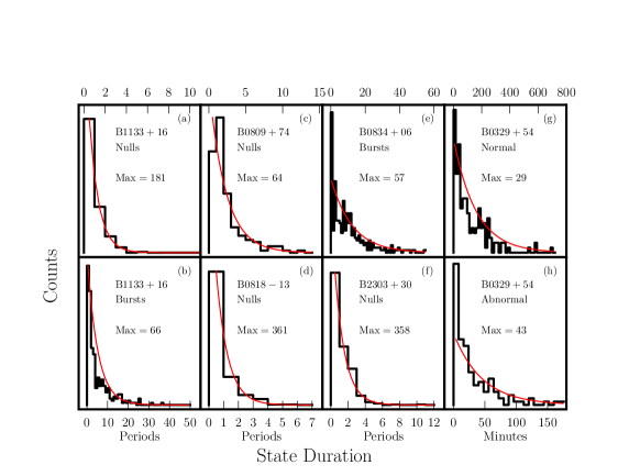
Figure 1: Histograms of durations of nulls, bursts, and modes for six pulsars. Frames (a) and (b) show null and burst histograms for B1133+16 at 325 MHz from Bhat et al. (2007); (c) Nulls for B0809+74 at 350 MHz (van Leeuwen et al., 2002); (d) Nulls for B0818-13 (Janssen & van Leeuwen, 2004); (e) Bursts for B0834+06 (Redman & Rankin, 2009); (f) Nulls for B2303+30 (Redman et al., 2005); (g) and (h) Normal and abnormal mode durations for B0329+54 (Chen et al., 2011). The smooth lines are Equation 1 evaluated using the mean state duration and the number of counts in each case; they are not least-squares fits and are given solely as fiducial examples. The maximum number of counts is given in each frame.

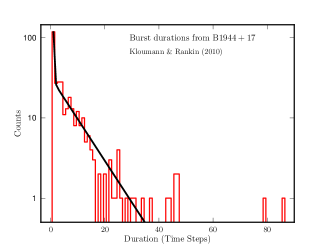
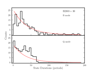
Figure 2: Left: Histogram of burst durations for B1944+17 at 327 MHz (after Kloumann & Rankin 2010). The solid line shows the predicted distribution for a four-state Markov model where two burst states are counted together as discussed in the text (Section 4.2). Right: Histograms of the durations of the burst (B) and quiet (Q) modes for B2303+30 from Redman et al. (2005). The smooth lines are Equation 1 evaluated using the mean state duration and the number of counts in each case.

Table 1: State Change Phenomena in Pulsars

Phenomenon	Properties	Number of	Examples	References
		States
Nulls and bursts	On:off flux density ratio $\gtrsim 100$.	2 to 4	B0031$-$07	1,2,3
	Null fractions: $f_{n}\leq 94$%.		B1237+25
	Durations $\lesssim 1$ s to hours.		B1944+17
	Residence time PDFs:		B0826-34	4, 5
	1. broad, monotonic
	2. dual components (often).
Mode changes	Changes in average pulse shapes.	2 to 3	B0329+54	6,7
			B1237+25
Subpulse drifts	Systematic pulse-phase drifts	$\leq 4$	B0031$-$07,	8,9,10
	through pulse window.		B1822$-$09
	Preferred drift rates.		B1944+17
	Allowed, forbidden state sequences.		B2319+60
	Mixed with unorganized drift states.
	Quasi-periodicities in $\gtrsim 55$% of pulsars.			10, 11
Long-term intermittency	Off states: hours to years.	2	J1832+0029	12
	Torque 1.5 to 2.5 times larger in on state.		J1841$-$0500	13
	38-day quasi-periodicity in B1931+24		B1931+24	14, 15
Profile and torque changes	Correlated mode and torque changes.	$\gtrsim 2$		16
	Month-like time scales.
Radio/X-ray correlation	X-ray on-off state transitions	2	B0943+10	17
	correlate with radio modes.
Extreme bursts	Giant pulses.	2	Crab pulsar	18
			(J0534+2200)
	Sporadic bursts with underlying period.	2	Rotating radio	19,20,21,22
			transients

References. — 1. Ritchings (1976); 2. Biggs (1992); 3. Deich et al. (1986); 4. Kloumann & Rankin (2010); 5. Gajjar et al. (2012); 6. Bartel et al. (1982); 7. Wang et al. (2007); 8. Huguenin et al. (1970); 9. Wright & Fowler (1981b); 10. Backer (1973); 11. Weltevrede et al. (2006); 12. Lorimer et al. (2012); 13. Camilo et al. (2012); 14. Kramer et al. (2006); 15. Young et al. (2013); 16. Lyne et al. (2010); 17. Hermsen et al. (2013); 18. Lundgren et al. (1995); 19. McLaughlin et al. (2006); 20. Deneva et al. (2009); 21. Keane et al. (2011); 22. Palliyaguru et al. (2011).

3 Markov and Stochastic Resonance Models

The broad, exponential-like distributions for state changes, along with the lack of any correlation between adjacent null and burst durations, are naturally explained by pulse sequences that conform to an underlying Markov chain. So too is the inconsistency of nulls and bursts with the Wald-Wolfowitz ‘runs’ test (Redman & Rankin, 2009). An additional phenomenon — stochastic resonance — is suggested by the binary state switching in the long-term intermittent pulsar B1931+24. The durations of on-and-off states for this object also have wide distributions but they are neither exponential nor monotonic. In addition, an underlying period of $38\pm 5$ days is discernible in a 13-yr data set (Young et al., 2013). While sampling incompleteness may distort the distributions, the phenomena are indicative of stochastic resonance in a nonlinear system that has binary states and is driven by a forcing function that could be strictly periodic or itself quasi-periodic.

Along with binary states, some pulsars show multiple discrete values of subpulse drift rate or quasi-periods in pulse amplitudes. These have been compellingly associated with a carousel of sub-beams that rotate through the overall radio emission cone with circulation times of tens to hundreds of seconds (Deshpande & Rankin, 1999; Rankin & Stappers, 2008). The changes in drift rate or quasi-period, often combined with nulling, imply that some objects display at least four states. These are also easily describable as Markov chains but with some state transitions disallowed, as discussed below.

Our approach is to generally discuss observed state-switching in terms of Markov processes and stochastic resonance.

3.1 Markov Processes

Markov processes are summarized here with reference to Papoulis (1991). We consider $n$-state Markov processes (denoted $M_{n}$) that have state values $\boldsymbol{S}=\{s_{1},s_{2},\cdots,s_{n}\}$. Transitions between states are described by an $n\times n$ stochastic matrix $\boldsymbol{Q}$ whose elements are the probabilities $q_{ij},i,j=1,\ldots,n$ for changing from state $s_{i}$ to state $s_{j}$ in a single time step. For observations we discuss, the time step is a single rotation period. Normalization across a row is $\sum_{j}q_{ij}=1$ and the probability for staying in the $i^{th}$ state is the “metastability” $q_{ii}$. The duration $T$ of the $i^{th}$ state is a random variable with probability $\propto q_{ii}^{T}$ for $T$ time steps, mean $T_{i}=(1-q_{ii})^{-1}$, and rms $\sigma_{T_{i}}=T_{i}\sqrt{q_{ii}}$. The probability density function (PDF) of $T$ for the $i^{th}$ state is given by $q_{ii}^{T}=(1-T_{I}^{-1})^{T}$ normalized by the sum of this quantity over all values of $T$, or

$$f_{T_{i}}(T)=T_{i}^{-1}\left(1-T_{i}^{-1}\right)^{T-1},\quad T=1,2,\cdots.$$ (1)

The PDF has constant slope $d\ln f_{T_{i}}(T)/dT=\ln(1-1/T_{i})$ and is generally steeper than an exponential that has the same mean, $T_{i}$. However, as $T_{i}\to\infty$ (or equivalently $q_{ii}\to 1$), the PDF tends to a one-sided exponential function with $\sigma_{T_{i}}=T_{i}$.

The ensemble probabilities of each state are given by the state probability vector $\boldsymbol{P}=(p_{1},p_{2},\cdots,p_{n})$. Stationarity, which we assume, requires that $\boldsymbol{P}\boldsymbol{Q}=\boldsymbol{P}$, so $\boldsymbol{P}$ is the left eigenvector of $\boldsymbol{Q}$ with unit eigenvalue. The transition matrix after $t$ time steps, $\boldsymbol{Q}^{t}$, converges to a form $\boldsymbol{Q}^{\infty}$ whose rows are all equal to the state probability vector. The convergence time is some multiple of the longest-duration state.

A two-state $M_{2}$ process with $\boldsymbol{S}=\{n,b\}$ for nulls and bursts, for example, has $p_{1,2}=T_{1,2}/(T_{1}+T_{2})$. The nulling fraction equals $p_{1}$ and can be written as

$$f_{n}=\frac{T_{1}}{T_{1}+T_{2}}=\frac{1-q_{22}}{2-q_{11}-q_{22}}=\frac{q_{21}}{q_{12}+q_{21}},$$ (2)

making explicit that $f_{n}$ can be identical for objects that have markedly different mean state durations, as observed. Examples of two-state Markov processes in Figure 3 (top three rows) show the dependence of the time series and state-duration histograms on the metastabilities $q_{11},q_{22}$.

To model a time series, the number of states and the transition matrix need to be determined. There are $n(n-1)$ unique elements in $\boldsymbol{Q}$ for an $n$-state process, after accounting for normalization across rows. Of these, $n$ elements can be determined from the mean state durations, $T_{i},i=1,\dots,n$. Frequencies of occurrence of the states constrain an additional $n-1$ elements. The remaining $n(n-3)+1$ elements need to be obtained using additional assumptions or measurements. For $n=2$, the system can be determined solely from the mean state durations so measured frequencies of occurrence provide redundancy. For $n=3$, mean durations and frequencies need to be combined with one additional measurement is needed. We will also consider $n=4$ processes that require five additional elements.

3.2 Nonlinear Systems and Stochastic Resonance

Markov processes are often used to describe non-linear systems that have an underlying potential-energy function with minima corresponding to the Markov states (e.g. Becker & Rein ten Wolde, 2012). Random motions (‘noise’) within potential wells induce state changes at rates that depend on well depths and noise strengths. State changes can also be driven by a forcing function that itself is stochastic, chaotic, or deterministic (Anishchenko, Anufrieva & Vadivasova, 2006). A strictly periodic forcing function acting in concert with noise can induce state changes that are only quasi-periodic (Gammaitoni et al., 1998), a phenomenon known as stochastic resonance.

When driven by both noise and a forcing function $d(t)$, a system potential having two local minima separated by a barrier can be described as an $M_{2}$ process in the adiabatic regime where $d(t)$ is slowly varying. The transition matrix is

$$\boldsymbol{Q}=\left(\begin{array}[]{cc}1-q_{12}e^{A_{1}d(t)}&q_{12}e^{A_{1}d(t)}\\ q_{21}e^{-A_{2}d(t)}&1-q_{21}e^{-A_{2}d(t)}\end{array}\right),$$ (5)

where $A_{1,2}\geq 0$ depend on properties of the wells and noise. Generally, the process is non-stationary. For $A_{1,2}=0$, $\boldsymbol{Q}$ reverts to the form for a simple $M_{2}$ process with time independent elements. Later we consider periodic forcing with $d(t)=\cos(2\pi t/P_{\rm f}+\phi)$ where $P_{\rm f}$ is the period and $\phi$ is an arbitrary phase. Over a cycle of $d(t)$, the well depths oscillate with the two wells out of phase by $\pi$.

Examples of two-state Markov processes in Figure 3 with different degrees of stochastic resonance (bottom three rows) show how state-duration histograms depend on the system parameters. Unlike the top three rows that show exponential-like histograms, stochastic resonance makes the histograms non-monotonic and periodic. Power spectra shown in the right-hand panels are featureless in the top three rows but show a spectral line to varying degrees in the bottom three rows at a frequency $\sim 20$ mcycles step^-1.

Figure 3: Time series, histograms of state durations, and power spectra for two-state processes. Left: single-realization time series for different values of the metastability probabilities $q_{11}$ and $q_{22}$ and for the stochastic resonance amplitudes $A_{1,2}$, as given in the top of each frame. The top three rows are for pure Markov processes ($A_{1,2}=0$) and the bottom three include a periodic forcing function with $A_{1,2}>0$ and period $P_{\rm f}=50$ time steps. Center: Histograms of the durations of low states and high states states based on 5000 realizations of the time series. The logarithmic vertical scales are from 1 to $10^{5.4}$. Right: Power spectra averaged over 5000 realizations plotted up to one-half the Nyquist frequency. The logarithmic vertical scale ranges from $10^{-7}$ to 0.1. The 50-step period for the stochastic resonance in the lower three panels is evident to varying degrees as a spectral line at a frequency of 20 milli-cycles step^-1.

4 Application to Short-term Nulling and Pulse-Profile Mode Changes

Nulls and bursts are often described empirically as two-state phenomena and so are some pulse-shape ‘mode’ changes. The null fraction appears to be characteristic of a pulsar and is constant over decades in well-studied objects, suggesting that the transition matrix in a Markov model is stable in the same manner as the average pulse profile. Histograms of state durations are almost always broad and monotonically decreasing (Deich et al., 1986; Redman et al., 2005; Bhat et al., 2007; Kloumann & Rankin, 2010; Chen et al., 2011; Gajjar et al., 2012) with many (e.g. B0835$-$41, B1112+50, B1133+16, B2111+46, B2303+30) showing consistency with the exponential-like form expected for an $M_{2}$ Markov process.

Null and burst sequences fail the Wald-Wolfowitz ‘runs’ test that is predicated on transitions occurring independently of the current state, as in coin tossing (Redman & Rankin, 2009) or any independent, identically distributed (i.i.d.) process. Coin tossing corresponds to a Markov process whose transition matrix $\boldsymbol{Q}$ has identical rows. However, transition matrices consistent with observed nulls and bursts necessarily have different rows and will fail the runs test. The test statistic used for the runs test is $Z=(R-\langle R\rangle)/\sigma_{R}$ (Redman & Rankin, 2009), where R is the length of a null or burst; $Z$ has zero mean and unit variance for an i.i.d. process. In general an $M_{2}$ process has mean $\langle Z\rangle=\sqrt{N}(T_{1}^{-1}+T_{2}^{-1}-1)=\sqrt{N}\left[(1-f_{n})T_{1}^{-1}-1\right]$ where $N\gg 1$ is the number of pulses analyzed. An i.i.d. process has $T_{1}^{-1}+T_{2}^{-1}\equiv 1$ so that $\langle Z\rangle=0$. However a Markov process with nulling fraction $f_{n}=0.32$ and $N=1024$ pulses (an example in Redman & Rankin (2009)) yields $\langle Z\rangle=-27.3$. It is noteworthy that estimates of $Z$ for 25 out of 26 pulsars range between -0.5 and -43 (Redman & Rankin, 2009; Gajjar et al., 2012), as expected for an $M_{2}$ process that accounts for the observed state durations.

4.1 False Transitions from Measurement Noise and Beaming

In this section we consider the effects of misidentified state transitions that inevitably result from measurements with finite S/N. Coherent emission from pulsars typically shows a broad pulse-amplitude distribution (e.g. Gajjar et al., 2012, Figure 2), often taking a log-normal form (e.g. Burke-Spolaor et al., 2012) for the phase-integrated intensity and in some cases a power-law form (e.g. Lundgren et al., 1995; Cognard et al., 1996; Cordes et al., 2004).

A model for the averaged intensity (pulse ‘energy’) in an on-pulse window is

$$I(t)=b(t)A(t|M_{2}(t))+N(t),$$ (6)

where $N(t)$ is white, Gaussian noise with variance $\sigma_{N}^{2}$ and $A(t|M_{2}(t))$ is a state-dependent pulse amplitude. The time-dependent beaming function $b(t)$ is a multiplicative factor that models pulse-to-pulse modulations caused by the entire radiation beam being only partially and stochastically filled with sub-beams or containing periodically spaced beams, as in the carousel model of Deshpande & Rankin (1999).

Letting the two states be $\boldsymbol{S}=\left\{0,1\right\}$, the pulse amplitude is

$$A(t|M_{2}(t)=\left\{\begin{array}[]{ll}0&M_{2}=0\\ a(\mu,\sigma)/\langle a\rangle&M_{2}=1,\end{array}\right.$$ (9)

where $a(\mu,\sigma)$ is a log-normal random variable with parameters $\mu$ and $\sigma$. When $M_{2}=1$, a statistically independent value is drawn for $a(\mu,\sigma)$ and normalized by the mean, $\langle a\rangle$. Defined this way, $\langle A(t)\rangle=1$ for the $M_{2}=1$ state and the average signal to noise ratio is $\rm S/N=\langle A\rangle/\sigma_{N}=1/\sigma_{N}$.

4.1.1 False Transitions from Additive Noise

First we consider the effects of additive noise when the beaming function is constant. Figures 4 and 5 show time series and histograms for simulations using Equation 6. In Figure 4 the low and high states are well separated so that additive noise does not affect the identification of the two states in a time series. Time series were generated according to Equations 6-9 using $\rm S/N=20$, $\mu=1.5$, and $\sigma=0.2$ and a threshold of $x=3\sigma_{N}$ was used to discriminate between low and high states. The lower S/N case in Figure 5 with $\rm S/N=10$, $\mu=0.8$, and $\sigma=0.5$ shows overlap between the two observable state amplitudes, with consequent misidentified transitions. These alter the duration histograms by adding many short nulls and shortening the durations of bursts, which respectively cause the narrow feature near $T=0$ in the inferred-null histogram and the steepening of the inferred burst histogram in the lower-right of the figure.

The false-transition probabilities for a threshold $x$ and for PDFs $f_{N}(N)$ and $f_{a}(a)$ for the noise and pulse amplitudes, respectively, are

$$r_{12} = \int_{x}^{\infty}dN\,f_{N}(N)$$ (10)

$$r_{21} = \int_{0}^{\infty}da\,f_{a}(a)\int_{-\infty}^{x-a}dN\,f_{N}(N).$$

Given the statistical independence of Markov transitions and noise-induced threshold crossings, the combined off-diagonal transition probabilities are (using ‘M’ to denote the noise-free Markov values)

$$q_{12}=q_{12,M}+r_{12}-q_{12,M}r_{12}\geq q_{12,M},$$ (11)

$$q_{21}=q_{21,M}+r_{21}-q_{21,M}r_{21}\geq q_{21,M},$$ (12)

showing that the interstate transition probabilities are always increased by additive noise, as expected.

For the case presented in Figure 5, $r_{21}>r_{12}$ because the Gaussian noise PDF falls off more rapidly for high values than does the log-normal PDF going to small values. This causes the spike at short durations to appear only in the null-duration PDF. For other choices of PDFs, S/N, and threshold, spikes can appear in one or the other (or both) of the null and burst PDFs .

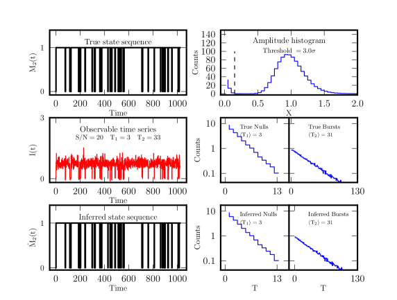
Figure 4: Simulated time series and histograms for a case where all pulse amplitudes are well above the threshold for dividing null and burst pulses. The left column shows a single time-series realization while the histograms in the right-hand column are based on 1000 realizations. Top left: time series of the Markov process. Middle left: time series of the intensity that includes additive noise and pulse-amplitude variations (Equation 6); the mean signal-to-noise ratio and mean state durations are indicated. Lower left: inferred state sequence obtained by identifying transitions in the intensity time series. Top right: histogram of pulse amplitudes; the dashed line represents the $3\sigma$ threshold for separating null and burst pulses. Middle right: histograms of the true durations of null and bursts states; the estimated mean durations are indicated. Bottom right: histograms of the null and burst durations inferred from the intensity.

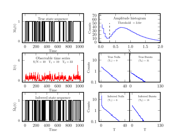
Figure 5: Same as Figure 4 but for a case where the pulse amplitude distribution and additive noise distributions overlap significantly.

4.1.2 Pseudo-Nulls from the Multiplicative Beaming Function

Kloumann & Rankin (2010, hereafter KL10) identified an excess number of short nulls and short bursts over what would be expected from an $M_{2}$ process having long mean state durations. Their physical explanation is that the excess short nulls are “pseudo” nulls resulting from the granularity of conal carousel beams while true nulls (both short and long) are caused by bona fide state changes, either a temporal cessation or a strong diminution of the radio intensity. This interpretation implies that the two processes (beaming and actual nulling) are independent and therefore multiplicative.

When the beaming function $b(t)$ is included in the intensity model of Equation 6 as a highly modulated quantity with minima well below the mean, the statistics of true nulls and bursts are modified. Short, pseudo nulls $\sim$one period in duration truncate bursts and therefore decrease the mean durations of both nulls and bursts while increasing their numbers in a time series. It can be shown that any modulation, periodic or otherwise, will have the same effect on the null and burst duration histograms. It is not so clear that beam modulations will have the analogous effect of producing short bursts unless there are occasional times when $b(t)$ is especially large for durations of one spin period (or less).

4.2 Dual-Component Nulls and Bursts

Several objects in addition to B1944+17 show dual characteristic durations for nulls or bursts. Some but not all short nulls and bursts with $\sim 1$ period durations could be caused by false transitions from additive noise or by pseudo-nulls due to multiplicative beaming variations, as discussed above.

Here we acknowledge such contaminating effects on null and burst statistics but proceed with a Markov description, which is certainly allowed no matter the cause of the various kinds of nulls and bursts. In particular, we demonstrate that the estimated distributions for null and burst durations can be accounted for by an $M_{4}$ process. The state set $\boldsymbol{S}=\{n_{1},n_{2},b_{1},b_{2}\}$ comprises two null states ($n_{1,2}$) and two burst states ($b_{1,2}$) that are not observationally distinguished, apart from their durations. To proceed, we adopt a minimalist model where transitions are allowed only between a null state and a burst state and vice versa but $n_{1}$ - $n_{2}$ and $b_{1}$-$b_{2}$ transitions in either direction are forbidden. Of the 16 equations needed to solve for the matrix elements, four come from normalization across rows, four from the mean state durations, and three from the frequencies of occurrence of the four states, which we estimate from information in KL10. The forbidden transitions are represented by four zero elements, so only one additional equation is needed. We estimated mean durations $(T_{1},T_{2},T_{3},T_{4})\approx(1.01,16.6,1.01,8.9)$ (in period units) and frequencies of occurrence for the four states, $\boldsymbol{f}=(f_{1},f_{2},f_{3},f_{4})\approx(0.01,0.655,0.013,0.321)$, from Figure 3 of KL10.

The full transition matrix was determined by searching over a grid of values for the off-diagonal elements, q13, q23, q31, and q41, while holding the diagonal elements $q_{ii},i=1,4$ fixed to values consistent with the mean durations and setting $q_{12}=q_{21}=q_{34}=q_{43}=0$. For each trial transition matrix $\boldsymbol{Q}$ we determined the state probability vector $\boldsymbol{P}$ from $\boldsymbol{Q}^{100}$ (as an approximation to $\boldsymbol{Q}^{\infty}$; see Section 3). By minimizing the mean-square difference $|\boldsymbol{P}-\boldsymbol{f}|^{2}$ we obtained a (non-unique) solution,

$$\boldsymbol{Q}_{(n_{1},n_{2},b_{1},b_{2})}\approx\left(\begin{array}[]{cccc}0.01&0&0.886&0.104\\ 0&0.940&0.006&0.054\\ 0.469&0.521&0.01&0\\ 0.012&0.100&0&0.887\end{array}\right).$$ (17)

The values of 0.01 for the metastabilities of short nulls and short bursts yield durations of order one time step, i.e. $T=1/(1-0.01)\sim 1$. Higher time resolution data can sharpen these values. Figure 2 (left) shows the Markov distribution that superposes the two burst states (properly weighted according to their frequencies of occurrence and durations) overplotted on the histogram of burst durations from KL10. The Markov distribution is a good representation of the salient features of the histogram. There may be an excess of observed long bursts compared to the observed counts, but they are small in number; some of these may result from short nulls that are missed in some of the data (i.e. false non-transitions).

As implied in our merging of the two burst states, the four-state description for B1944+17 can be reduced to a three-state description if short and long nulls are combined into an $\boldsymbol{S}=\{n,b_{1},b_{2}\}$ model or bursts combined into an $\boldsymbol{S}=\{n_{1},n_{2},b\}$ model. Similar 3-state descriptions can account for the dual nulling patterns seen from pulsars B0809+74 (van Leeuwen et al., 2002; Gajjar et al., 2012); B0818$-$13 (Janssen & van Leeuwen, 2004); J0828$-$3417, J0941$-$39, and J1107$-$5907 (Burke-Spolaor et al., 2012); B0835$-$41, B2034+19, B2021+51, and B2319+60 (Gajjar et al., 2012). The object B0826$-$34 shows a null state with occasional single pulses and a burst state with rare single-pulse nulls (Esamdin et al., 2012) for which the average pulse shapes in these states differ significantly. This object is also amenable to a Markov description but a quantitative description of state durations and fractions is needed.

4.3 Subpulse Drift Modes

In some pulsars, there are well-organized motions of subpulses across the pulse-phase window defined by averages of a large number of pulses. Two or three subpulses typically appear in a single pulse period with separation $P_{2}$, usually expressed in time units. In a sequence of pulse periods, bands of drifting subpulses have separations $P_{3}$ at fixed pulse phase, usually expressed in units of the spin period $P$. The drift rate is then $P_{2}/P_{3}$ or, in physical units, $\dot{\phi}=P_{2}/P^{2}P_{3}$ cycles s^-1 when $P_{2}$ and $P$ are expressed in time units and $P_{3}$ in spin periods. A common interpretation is that drifts correspond to $\boldsymbol{E}\times\boldsymbol{B}$ motions of multiple particle and radiation beams (a beam ‘carousel’) around a magnetic axis or some other related axis (Ruderman & Sutherland, 1975; Deshpande & Rankin, 1999; Gil et al., 2006; Li et al., 2012b). The total time needed for a beam to circulate around the axis is $P_{4}=1/\dot{\phi}P=PP_{3}/P_{2}$ in units of spin periods. While $P_{2}$ and $P_{3}$ are visually recognizable in pulse sequences for some pulsars, the circulation time $P_{4}$ is often inferred from power spectra of pulse intensities at a single pulse phase (Backer, 1973; Wright & Fowler, 1981b; Deshpande & Rankin, 1999; Weltevrede et al., 2006). For some objects discussed below, the drift pattern can have variable $P_{3}$ and $P_{4}$ but with near constancy of $P_{2}$.

When in the ‘on’ state, B1944+17 shows additional complexity in the form of four different emission modes (Deich et al., 1986, KL10) that are distinguished by different subpulse drift rates or average pulse shape. Combined with nulling described above, as many as ten states may be needed for a full description, but additional observational classification is needed for any detailed modeling.

Two pulsars that show three distinct drift rates along with nulls are B0031$-$07 (Huguenin et al., 1970; Wright & Fowler, 1981a; Vivekanand & Joshi, 1997) and B2319+60 (Wright & Fowler, 1981b). The states are labelled A, B, and C in order of increasing drift rate. For B0031$-$07, the drift rates have ratios 1:1.9:2.8 and observed sequences include B only and hybrid AB and BC bursts. There are no A only or C only bursts, or AC, BA, CA, or CB combinations. A four-state model $\boldsymbol{S}=\{n,A,B,C\}$ will have a transition matrix with $q_{nC}=q_{An}=q_{AC}=q_{BA}=q_{CA}=q_{CB}=0$ and six remaining unique values need to be determined from measurements. Three can be obtained from the frequencies of occurrence $\boldsymbol{f}=(f_{n},f_{A},f_{B},f_{C})\approx(0.45,0.086,0.45,0.014)$ and the four diagonal elements from the as-yet unknown mean durations of each state. Future measurements can allow determination of the full matrix with one redundant estimate that can be used as a check. Our discussion comprises an existence proof for a Markov model because, even without knowing the diagonal elements of $\boldsymbol{Q}$, it provides the mechanism for ‘forbidden’ transitions as well as the allowed transitions.

Very similarly, B2319+60 has A,B, and C states that display different drift rates and pulse shapes along with nulls occurring with $\boldsymbol{f}=(f_{n},f_{A},f_{B},f_{C})\approx(0.3,0.45,0.15,0.1)$. However, there are more allowed sequences than for B0031$-$07, so eight unique elements of the transition matrix need to be determined after setting $q_{AC}=q_{BA}=q_{CA}=q_{CB}=0$. Seven can be estimated from the mean state durations (currently not in the literature) and $\boldsymbol{f}$. The eighth can be obtained by estimating the number of AB or BC transitions.

A remarkable feature of state transitions in both B0031$-$07 and B2319+60 is that subpulse drift states occur only in order of increasing drift rate. In the carousel model, the drift rate is related to the local plasma drift velocity $c\boldsymbol{E}\times\boldsymbol{B}/B^{2}$ that vanishes when the local charge density equals the Goldreich-Julian density. An increasing drift rate therefore suggests depletion of the charge density over the course of a burst that eventually terminates in a null. In a nonlinear model, the systems in these two pulsars seem to be running ‘downhill’ in an effective potential that is somehow reset during and perhaps because of a null. The A, B, and C states would have energy minima such that it is much more likely to have AB, BC, and AC transitions than BA, CB, or CA transitions.

4.4 Mode Changes with Long Time Constants

Two pulsars show pulse-shape modes that have finite time constants for the evolution of the drift rate in one of the modes. The exemplar drifting-subpulse object B0809+74 has 1.4% null pulses that interrupt bursts (Lyne & Ashworth, 1983; van Leeuwen et al., 2002). Like other objects, the durations of nulls and bursts have Markov distributions, but during bursts the drift rate decreases at the onset of a null and relaxes exponentially to a larger asymptotic value over a time that scales with the null duration but is typically tens of seconds (Lyne & Ashworth, 1983).

The B and Q burst modes from B0943+10 (Rankin & Stappers, 2008) can be accommodated by a two-state Markov process but with some complications. This pulsar displays correlated X-ray and radio states that, along with torque variations seen in other pulsars, link radio and high-energy phenomena (Hermsen et al., 2013). The two burst-only radio states show a quasi-period $P_{4}$ that is constant in the weaker Q mode but evolves exponentially with a 73 min time constant in the B mode. As $P_{4}$ increases the pulse shape changes progressively on the same time scale. The exponential increase in $P_{4}$ (equivalent to a decrease in drift rate) suggests in the carousel model that, unlike for B0031$-$07 and B2319+60 discussed above, the $\boldsymbol{E}\times\boldsymbol{B}$ drift velocity decreases in B-mode sequences, implying that the polar-cap acceleration region trends toward a force-free state. In the ionic evolution model of Jones (2011), the vertical potential drop in the polar-cap accelerator evolves as high-Z ions are increasingly ionized and disassociated. It is not clear in either of these interpretations why the state changes are not more periodic rather than showing a wide range of durations, but a nonlinear system driven stochastically can account for these.

5 Long-term Intermittency and Stochastic Resonance

Three objects (J1832+0029, J1841-0500, and B1931+24) show distinct on and off emission states that are accompanied by switching between two values of the spindown rate $\dot{\nu}$. Thus far there are no detailed descriptions of pulse variations in the on state because intensity and timing results have been based on average profiles rather than single pulses.

The best studied object, B1931+24, shows no short-term nulls (minutes or less) when the pulsar is in the long-term ‘on’ state (Kramer et al., 2006). The durations of ons and offs have mean values of $8\pm 4$ d and $22\pm 7$ d and large maximum to minimum ratios, 19:1 and 10:1, respectively (Young et al., 2013). These ratios are similar to those of short-term nulls and bursts for other objects and, along with the lack of correlation between the durations of contiguous on-state and off-states, are consistent with a Markov description.

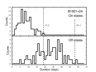
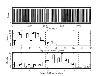
Figure 6: Left: Histograms of on-and-off state durations for B1931+24, after Figure 2 of Young et al. (2013). Vertical dashed lines indicate one-half and a full period of $P_{i}=38\pm 4$ d identified in a 13 y data set (Young et al., 2013). Right: Time series of state changes and histograms or state durations for a stochastic resonance model of the form of Equation 5 with $q_{11}=0.985,q_{22}=0.83,A_{1}=2.6,A_{2}=1.6$, and $P_{f}=38$ d.

However, the histograms of state durations are inconsistent with the monotonic form expected from a Markov process. As shown in Figure 6 (left panel), based on Figure 2 of Young et al. (2013) (see also Figure 1c of Kramer et al. (2006)), the mean state durations are about equal to their modes, and there is a paucity of short durations. The overall small number of on-off cycles in the 13-yr data set combined with sampling incompleteness (from allowing observation gaps as large as 5 d in the analysis, Young et al. (2013)) may contribute to the on-state histogram shape. Conversely, the deficit of off-state durations up to $\sim 15$ d is not plausibly accounted for this way.

Another difference from fast intermittency and Markov behavior is an apparent underlying period for the intermittency, $P_{\rm i}=38\pm 5$ d, in the 13 yr data span (Young et al., 2013) that is longer than any of the individual on-and-off durations and is about 4.8 times the mean on-duration and 1.7 times the mean off-duration. The quasi-periodicity may be interpreted in two ways. First, there may be a strictly periodic — but hidden — process that is blurred by mediating processes that lead to observable quantities. Alternatively, the 38 d period may be the mean of a process that is intrinsically quasi-periodic. We explore the first of these options because it is more specific.

A stochastic-resonance model is an acceptable statistical description of observations of B1931+24 if we adopt a transition matrix (Equation 5) with a sinusoidal forcing function $d(t)=\sin(2\pi t/P_{f}+\phi)$. In this interpretation the different mean on-and-off durations $T_{\rm on},T_{\rm off}$ signify an asymmetric effective potential and their sum, $T_{\rm on}+T_{\rm off}=31\pm 8$ d, is nominally smaller than the observed mean period $P_{i}=38\pm 5$ d reported by Young et al. (2013). Schmitt triggers show similar behavior when the underlying potential has asymmetric minima (Marchesoni, Apostolico & Santucci, 1999).

The right-hand panel of Figure 6 shows state-duration histograms for a stochastic-resonance model that is consistent with the observed histograms in the left-hand panel. The simulations include a strictly periodic forcing function with $P_{f}=P_{i}$. The centroids of the dominant features in the simulated histograms straddle the half period $P_{f}/2=19$ d, as is common in SR models. There is an additional feature in the simulated off-state histogram for durations $\lesssim 7$ d that may be absent in the actual data because of the incomplete sampling of short-duration states (Young et al., 2013) and because the total number of counts is smaller than in the simulated histogram. A more precise test of stochastic resonance in B1931+24 would require longer, continuous data sets than are currently available. Data sets that include single-pulses would be valuable for characterizing any very short-duration on or off states.

The other two objects that show long-term intermittency and discrete values of $\dot{\nu}$, J1832+0029 and J1841-0500, have state durations that are longer than those in B1931+24 and have not been sampled adequately to test whether a stochastic resonance model might apply to them as well.

6 Timing Variations from a Two-State Markov Process

Objects that are intermittent on long time scales like B1931+24 show a distinct value of spindown rate $\dot{\nu}$ in each state. Switching between discrete values of $\dot{\nu}$ can be viewed as pulse-like changes in $\dot{\nu}$ (i.e. equal upward and downward transitions) that combine with a constant value of $\dot{\nu}$, where we assume that the second derivative $\ddot{\nu}$ from the spindown torque is negligible. Viewed collectively as a two-state Markov process, switching between spindown rates produces a random walk in spin frequency and an integrated random walk for pulse phase. Stochastic timing variations occur because individual states last for times that vary widely about their means, as discussed earlier. We integrate the fluctuating part of $\dot{\nu}(t)$ twice to get the spin phase perturbation and calculate its variance over a data span of length $T_{d}\gg\overline{T}$ . Using the ‘reduced’ duration, $\overline{T}=T_{1}T_{2}/(T_{1}+T_{2})$, the rms timing variation expressed in time units can be written as

$$\sigma_{t,2}(T_{d})=C_{2}^{-1}\sigma_{t}(T_{d})\approx 74~{}\mu s\,P\,|\dot{\nu}_{-15}|\,\overline{T}_{3}^{1/2}T_{d,yr}^{3/2}\left|\frac{\delta\dot{\nu}}{\dot{\nu}}\right|\frac{\sqrt{f_{l}(1-f_{l})}}{1/2}.$$ (18)

In this equation, we have used $\overline{T}=10^{3}\overline{T}_{3}$ s, $T_{d}$ is in years, and $\dot{\nu}=\dot{\nu}_{-15}10^{-15}$ s^-2. The factor $C_{2}\approx 15.5$ corrects for the fluctuations removed by subtraction of the second-order polynomial fit for the mean spin rate and $\dot{\nu}$. All else being equal, the rms timing error is a maximum for equal fractions of low and high states, $f_{l}=f_{h}=1-f_{l}=1/2$. The scaling, $\sigma_{t}(T_{d})\propto T_{d}^{3/2}$, is generic to random walks in spin frequency (Groth, 1975; Cordes & Downs, 1985; Shannon & Cordes, 2010).

For B1931+24, individual transitions can be identified and removed from the data to reduce the rms timing variation (Kramer et al., 2006). However for other objects, individual states may not be identifiable because they are too small or are mixed with other spin variations and consequently will appear as spin noise with nonstationary variance.

7 Medium-term Intermittency and Timing Variations in B0823$+$26

B0823+26 ($P=0.53$ s and $\dot{\nu}=6\times 10^{-15}$ s^-2) displays minute-duration nulls along with those of hours and longer. Any emission during nulls is less than 1% of the mean on-state flux density. The distribution of on-state durations shows both a narrow and a broad component with times scales of minutes and days, respectively (Young et al., 2012). The durations of particular nulls and bursts may be mis-estimated in some cases due to data windowing effects that cause state changes to be missed, as noted by Young et al. (2012), but the presence of both long and short nulls is secure.

Torque variations are evidently more complex in this object than in long-term intermittent objects like B1931+24. In a 153-d data set, Young et al. (2012) saw neither cubic structure in the timing residuals above an rms residual of about 200$~{}\mu s$ nor switching between discrete values of $\dot{\nu}$ like that seen in B1931+24. The upper bound on the amplitudes of such pulses is $\Delta\dot{\nu}/\dot{\nu}\lesssim 0.06$ (Young et al., 2012) based on detailed modeling of the time series. What are seen in a longer data set, however, are step-function-like changes in $\dot{\nu}$ (rather than pulses) with amplitudes as large as $|\Delta\dot{\nu}/\dot{\nu}|=0.02$ but occurring at a rate of only $\sim 1.2$ yr^-1 (Cordes & Downs, 1985), much less frequent than the state changes discussed here.

We can place an additional statistical limit on the amplitudes of pulses in $\dot{\nu}$. Equation 18 with $p_{1}=0.2$, $T_{1}=0.26$ d and $T_{2}=1.4$ d (Young et al., 2012) predicts $\sigma_{t,2}(153~{}\rm d)\approx 610~{}\mu s~{}|\delta\dot{\nu}/\dot{\nu}|.$ Comparison with the upper bound of 80 $\mu s$ on the rms residual (c.f. Figure 8 and discussion in Young et al. (2012)) implies $|\delta\dot{\nu}/\dot{\nu}|\lesssim 0.13$, a less stringent constraint than $|\delta\dot{\nu}/\dot{\nu}|\lesssim 0.06$ obtained by (Young et al., 2012) from direct fitting. Using the smaller upper bound, we estimate that for a 13.6-year data set like that analyzed by Cordes & Downs (1985), state changes would produce no more than $\sigma_{t,2}(13.6~{}\rm yr)\approx 6.7~{}ms$, much smaller than the measured value of $\sim 100$ ms over this data span. Spin noise in B0823+26 is evidently dominated by step functions in $\dot{\nu}$ that yield a scaling $\sigma_{t}(T_{d})\propto T_{d}^{5/2}$, much steeper than that expected from pulses in $\dot{\nu}$. The origins of the step functions in $\dot{\nu}$ for B0823+26 appear distinct from the process that causes large pulses in $\dot{\nu}$ for B1931+24 (Kramer et al., 2006).

From the timing analysis on B0823+26 we conclude the following. First, switching between nulls and bursts on time scales of days evidently is not associated with large jumps between binary values of $\dot{\nu}$, the same conclusion as reached by Young et al. (2012). Second, the large amount of spin noise appears to have other causes than those that are responsible for the intensity jumps. The difficulty in identifying discrete values for $\dot{\nu}$ in B0823+26 may result from a two-state model being too simplistic. Any correlated torque events might also have different shapes than pulse-like forms. If the torque does not return to its original value (as it does in B1931+24 and other intermittent pulsars), the spin noise will appear more like that observed. Multiple states are also implied by the presence of nulls and bursts that each have short and long-duration components. A timing analysis of multiple state models is beyond the scope of this paper but is worthy of future analysis.

8 The Physics of Discrete States and Triggering Between States

The aggregated observational results presented in this paper demonstrate that diverse phenomena result from the existence of metastable states in the dynamics of pulsar magnetospheres. A physical understanding of the phenomena leads to two primary questions: (1) What is the underlying magnetospheric physics of the observed states? and (2) What causes transitions between states? We discuss these questions in the context of standard ideas about pulsar magnetospheres.

Some characteristic light-travel times associated with neutron stars (NSs) and their magnetospheres are useful for the following discussion. The NS radius is $R_{*}\sim 30~{}\mu s$ and the radius of the PC is $r_{\rm pc}=R_{*}(R_{*}/r_{\rm lc})^{1/2}\sim 0.5P^{-1/2}~{}\mu s$ for spin periods $P$ in seconds, where the light cylinder radius $r_{\rm lc}=cP/2\pi\sim 0.16P~{}s$. In models with an acceleration region just above the PC, the height of the region $h\lesssim r_{\rm pc}$ and for objects with sustained pair cascades, $h\sim 0.3~{}\mu s$. Radio intensity variations are seen on these and smaller time scales. Indeed, a priori one might expect all observed time scales to be no larger. However, the variations discussed in this paper concern macroscopic scales that exceed the characteristic times by many orders of magnitude (seconds to years) but are still much smaller than the spindown time $\tau_{s}=P/\dot{P}\sim 10^{7.2}P\dot{P}_{-15}^{-1}$ yr on which the magnetosphere evolves (where $\dot{P}=10^{-15}\dot{P}_{-15}$ s s^-1 is the period derivative). Thermal time scales enter the picture when thermionic emission plays a role and the temperature of a hot PC is time variable. Also, in some situations, pair cascades are temperature dependent (Hibschman & Arons, 2001; Medin & Lai, 2007). The heating and cooling times of the PC are estimated to be $\lesssim 1$ s and thermostatic regulation from pair production may result in variations on some multiple of this time scale (Cheng & Ruderman, 1980). Surface physics introduces the proton drift time through the atmosphere $\tau_{p}\sim 0.1$-1 s and the ‘excavation’ time for removing one radiation length’s amount of material from the PC, $\tau_{\rm rl}\approx 2.1\times 10^{5}~{}s~{}(P/ZB_{12})$ (Jones, 2011, 2012). Orbital periods around a 1.4 $M_{\odot}$ NS are $P_{\rm orb}\approx 127~{}s\,P^{3/2}(r/r_{\rm lc})^{3/2}$ using $r_{\rm lc}$ as a fiducial radius. An object with a 38 d orbital period at $r\sim 0.3$ AU is well outside the gravitational tidal disruption radius, $r_{tg}=(3M_{\rm NS}/2\pi\rho)^{1/3}\sim 10^{11}\rho^{-1/3}$ cm. Small objects inside the tidal radius can exist owing to tensile forces.

Radio emission requires relativistically beamed, coherent radiation from a particle flow that is collimated in a narrow, magnetic field-line bundle. Coherence is produced by an instability that requires counterstreaming particle flows and has a maximum growth rate at an altitude-dependent plasma frequency. Also required is a favorable viewing geometry that depends on the angular width of the radiation beam, which varies with altitude, and on the angle between the beam and the observer’s direction. The observed discrete states therefore require changes in one or more of these elements to alter the intensity, pulse shape, and spectrum of the radiation. That discrete states are seen in the dominant energy loss channels — viz. spindown rates $\dot{\nu}$ in the long-term intermittent pulsars like B1931+24 and X-ray emission from B0943+10 — implies that significant, discrete changes occur in the magnetosphere at large.

8.1 Metastable States

Several gross features of pulsar magnetospheres could provide binary states, including on-and-off modulation of $e^{\pm}$ production, cycling of the relative contributions of ions and pairs to the current flow, or modulations of the total current itself between two extremes, such as a vacuum state (no current) and a force-free state (e.g. Li et al., 2012b, c). Another dyadic pair could be a dead, ‘electrosphere’ state (e.g. Michel, 1980; Krause-Polstorff & Michel, 1985; Smith et al., 2001; Pétri et al., 2002) vs. a standard, dynamic magnetosphere. Extreme switching between an electrosphere and a magnetosphere might be associated with the more extreme RRATs and long-term intermittent objects (e.g. Michel, 2010).

Observed state changes so far are exclusively the realm of older, canonical pulsars with periods $\gtrsim 0.3$ s and magnetic fields $B\sim 10^{12}$ G. Indeed, there appears to be a greater propensity for state changes in pulsars that are longward of $\sim 0.3$ s in the $P$-$\dot{P}$ diagram (Figure 1, Cordes & Shannon, 2008). However, it is conceivable that shorter period objects display state changes that have been missed because of observational selection, particularly MSPs for which there are few observations of single pulses. Whether any state changes are expected from MSPs depends on the nature of the states themselves and on how state changes are triggered. If one of the state dyads is associated with a threshold for pair production, state transitions will be expected if the pair-production death line is near the MSP population in the $P$-$\dot{P}$ diagram. Published death lines do not provide clarity on this because they depend on the types of current flow (SCL or not), on the photon-emission process (curvature vs. inverse-Compton) (Hibschman & Arons, 2001; Harding et al., 2002; Wang & Hirotani, 2011; Harding & Muslimov, 2011; Medin & Lai, 2007), and on any offset of PCs from the dipole axis caused by current-driven sweepback of the magnetic field (Harding & Muslimov, 2011) or by an offset dipole (e.g. Hibschman & Arons, 2001). If alternative photon-processes can drive pair cascades for different regions in the $P$-$\dot{P}$ diagram, the propensity for state changes may be associated with just one of the processes, such as non-resonant inverse Compton radiation vs. curvature radiation.

8.2 State Triggering

A model is proposed in which the dynamics of current flows are responsible for both defining discrete states and for causing transitions between them. In this picture, spindown rates and X-ray states, along with radio nulling, drifts, and mode changes, are all collateral effects. Discrete states are tied to the physics of the magnetic polar cap (PC) while switching involves both local and global effects. The suitability of simple Markov processes for describing the distributions of state durations in most cases suggests that state switching is largely stochastic. This is most easily understood as self-driven stochasticity of the acceleration region. The natural time scale for such variations $\lesssim 1~{}\mu s$. However, the stochastic resonance model for the quasi-periodicity in B1931+24 suggests the action of a forcing function with a long period $\sim 38$ days that is easiest to understand in terms of modulation of the return current from an equatorial disk outside the light cylinder. Equatorial disks are a common feature in recent discussions of magnetospheres and in numerical simulations of pulsar magnetospheres (Krause-Polstorff & Michel, 1985; Contopoulos, 2005; Timokhin, 2010; Kalapotharakos et al., 2012; Li et al., 2012b, c) and have long been argued for by Michel (1980). Dramatic changes of magnetospheric structure by pulsar-disk interactions were a conclusion of Barsukov et al. (2009). Recent magnetosphere models incorporate a ‘Y’ point where current from a disk flows along the separatrix to both magnetic PCs (e.g. Contopoulos, 2005; Timokhin, 2006). This feature may provide the most direct feedback from a pulsar’s environment to its PCs.

8.3 Circuit Analogs

The NS surface and atmosphere at the PC and the acceleration region above have been likened to the idealized unidirectional current flow of a diode (e.g. Arons & Scharlemann, 1979; Thompson, 2008). The analogy has been extended to include resistivity, capacitance, and inductance in linear circuits (e.g. Shibata, 1991; Jessner et al., 2001; Xu et al., 2006) that, in principle, could show oscillations with well-defined time scales. However, nonlinear circuits can have metastable states with broad, Markov-type durations when state switching occurs from noise-like voltage variations. A nonlinear, real-world diode with a forward bias voltage, a back-biased capacitance, and a finite recovery time to a reversal from forward to backward bias can show universal chaotic behavior when driven sinusoidally (Rollins & Hunt, 1982). Nonlinear circuits are amenable to a Markov description when switching between states is rapid compared to the residence time in any state and when ‘microscopic’ dynamics within a state can be ignored compared to the step-size of the Markov chain (e.g. Becker & Rein ten Wolde, 2012). An asymmetric Schmitt trigger, which features hysteresis and nonlinearity, has unequal switching thresholds for positive and negative inputs. It shows Markov variations for a random-noise input but can show stochastic resonance when driven sinusoidally, behavior that is generic to any asymmetric bistable system (Marchesoni, Apostolico & Santucci, 1999).

NS and their magnetospheres differ substantially from laboratory circuits because voltage drops and current flows along field lines are not controlled but instead are dynamical quantities, providing a richer variety of possible phenomena.

Pulsar magnetospheres strive to be force free ($\boldsymbol{E}\cdot\boldsymbol{B}=0$) by filling themselves with space charge at the Goldreich-Julian (GJ) density $\rho_{\rm GJ}\approx-{\boldsymbol{\Omega}\cdot\boldsymbol{B}}/{2\pi c}$, where $\boldsymbol{\Omega}$ is the spin vector. Standard models for pulsars include a corotating magnetosphere with $\rho=\rho_{\rm GJ}$ and an open field line (OFL) region where charge is lost through a current density $J\approx c\rho_{\rm GJ}$, but $\rho=\rho_{\rm GJ}$ almost everywhere except in acceleration regions where $\boldsymbol{E}\cdot\boldsymbol{B}\neq 0$. The potential drop sustains the current flow that contributes to the spindown torque and, along with secondary particles, produces radio to gamma-ray emission. The OFL region and magnetic PC are defined self-consistently from the combined ambient stellar magnetic field and current-driven field; the latter, in turn, depends on boundary conditions imposed by the global structure of the magnetosphere (e.g. Kalapotharakos et al., 2012).

Recent simulations (Kalapotharakos et al., 2012; Li et al., 2012b, c) demonstrate exquisitely how the spindown rate depends on the magnetic flux threading the light cylinder and takes on limiting values for vacuum ($\rho=0$) and force-free ($\rho=\rho_{\rm GJ}$) conditions in the OFL region. Spindown rates in these limits differ by a factor of four for inclination angles of 45^∘, easily bracketing the 2.5:1 range seen in long-term intermittent pulsars. For active, steady pulsars the magnetosphere appears to find a configuration that lies between the force-free and vacuum solutions. However, there is no obvious mechanism for defining dual (let alone multiple) states in what appears to be a continuum for the resistivity, which is a free parameter in determining the type of magnetosphere (Li et al., 2012b, c).

We attribute discrete current states to changes in the relative contributions from ions, protons, electrons, and $e^{\pm}$ pairs. This situation applies to an $\boldsymbol{\Omega}\cdot\boldsymbol{B}<0$ geometry for the OFL region at the NS surface, the situation considered by Ruderman & Sutherland (1975) and Jones (2011, 2012, 2013), that requires positive charges above the PC. The opposite case with $\boldsymbol{\Omega}\cdot\boldsymbol{B}>0$ has comparatively uncomplicated electron flows that may not allow pair production and radio emission. However, if it does, state changes are not expected. The $\boldsymbol{\Omega}\cdot\boldsymbol{B}<0$ and $\boldsymbol{\Omega}\cdot\boldsymbol{B}>0$ cases may then account for the stark differences between pulsars having similar $P$ and $\dot{P}$. Positive charges include ions with a wide range of charge to mass ratios resulting from particle showers onto the polar cap (Jones, 2012) along with protons and any positrons produced in pair avalanches. One form of current self-regulation involves thermionic emission from a PC that is kept hot by backflowing electrons from $e^{\pm}$ pairs (Cheng & Ruderman, 1980). Small changes in temperature can change the ion current density $J_{i}$ exponentially if the current flow is not space-charge limited (SCL). In this case, cessation of $e^{\pm}$ production allows the PC to cool and $J_{i}$ will decrease. Unless another charge source can compensate, the voltage drop will increase while the spindown rate decreases. Coherent radiation that requires a substantial pair plasma will also shut off. With SCL flow, however, cessation of pair production will cause a radio null but without a large decrease in torque on the star.

8.4 Return Currents and Stellar Charge

Current outflow must be matched by a return current, at least on average, if the NS is not to become charged sufficiently to halt current outflow from the polar cap. While a disaster for explaining steady pulsar radiation, episodic charging and discharging is a plausible mechanism for intermittency because it could take little time (about one spin period) to switch between charge states. In some models the return current is from separated $e^{\pm}$ pairs created within the magnetosphere, while in others it originates from an equatorial disk exterior to the magnetosphere. If a mismatch develops between outflow and inflow, it will self regulate if pair production is robust as in high-field, fastly spinning pulsars. However, longer-period or weak-field pulsars that operate near the threshold for pair production, will have a higher propensity for state changes. It is therefore notable that fast states (classical nulling, drifting and mode changes), long-term intermittency, discrete torques, and X-ray states have been seen only in pulsars with $P\gtrsim 0.3$ s and are common for $P\gtrsim 1$ s. Furthermore, nulling is most visible in objects with small angles between the spin axis and magnetic moment (Biggs, 1992; Cordes & Shannon, 2008). Given both of these conditions, it is plausible that currents originating from an equatorial disk can drive the system into and out of a state of dormancy, at least as far as radio emission is concerned.

Return currents from an exterior disk, if highly episodic, will modulate activity at the PC as well as alter the structure of the magnetosphere (Barsukov et al., 2009). Depending on their constituency, they can also ‘dope’ the NS surface with ions that differ from those that drift to the top of the thin atmosphere from below (Jones, 2011), which are fractionated in charge-to-mass ratio by backflow electrons (Jones, 2012). In laboratory diodes with non-SCL current flow, the current density depends on the type of material as well as on the voltage drop (Goncalves, Barroso, & Sandonato, 2004). A similar effect may occur in pulsars where the charge carriers could be a state-dependent mixture of surface and backflow ions. Like any circuit, the current flow in the magnetosphere can halt altogether. With sufficient net charge, the combined electrostatic and induced potential drops can shut off the conventional PC accelerator by reverse biasing the system (Pétri et al., 2002).

These considerations suggest that if return currents originate from or are affected by a disk external to the light cylinder, the electrodynamics of the disk itself will be involved in state-change phenomena. Disk instabilities combined with perturbations from contaminating material (e.g. asteroids; Cordes & Shannon, 2008) may introduce a wide range of time scales, including orbital time scales. Some of these may be stochastic and others periodic. In addition, magnetic reconnection within the disk from magnetic fields with oppositive polarities above and below the disk can inject relativistic particles into the magnetosphere (e.g. Contopoulos, 2005; Komissarov, 2006; Timokhin, 2006).

8.5 Discrete Drift States

We associate fast state changes with the acceleration region just above the NS surface and atmosphere e.g. (Ruderman & Sutherland, 1975). Fast nulling and pulse-shape modes suggest alteration of the particle composition in current density and the number of secondary $e^{\pm}$ pairs. Preferred drift rates may be associated with changing numbers of sub-beams in a rotating carousel. The number of sub-beams is likely involved in determining the local charge difference $\Delta\rho=\rho-\rho_{\rm GJ}$ and thus would affect the $\boldsymbol{E}\times\boldsymbol{B}$ drift velocity. The number of carousel beams $\sim 20$ in B0943+10 (Deshpande & Rankin, 1999) while another object, B1822-09, appears to involve only two subpulse beams in B mode and three in Q mode (Latham et al., 2012). Sub-beam creation and annihilation would be an attractive process for producing discrete values of subpulse drifts and other state attributes. However, two pulsars mentioned earlier (B0031$-$07 and B2319+60) have approximately constant $P_{2}$ in the three observed drift modes in which there is an increase in $P_{3}$ and a decrease in the drift rate $P_{2}/P_{3}$. The spatial separation of sub-beams is directly related to $P_{2}$ suggesting, at least for these two objects, a constant number of sub-beams because $N_{sb}\propto P_{4}/P_{2}$. In other pulsars the variability of $P_{2}$ is not well constrained. An alternative to the rotating carousel model is the diocotron instability that has been suggested as a cause of subpulse drifts Fung et al. (2006), which results from differential angular rotation across the OFL region. Magnetospheric models that incorporate this instability are not well-enough developed to provide a basis for further discussion in this paper.

8.6 Long-lived States, Energetics, and MSPs

The range of time scales seen in pulsar intermittency is large so it is natural to ask what other time scales are relevant and what the energetics are. Given that observed time scales have little relationship to characteristic times of NS and their magnetospheres and that processes exterior to the magnetosphere may be involved, objects with much longer state durations (e.g. years, decades) plausibly exist that will be discovered in comprehensive radio surveys that have a large product of time coverage and field-of-view. (e.g. Macquart et al., 2010; Murphy et al., 2013).

As for energetics, it is well known that pulsar radio luminosities are only small fractions ($\sim 10^{-8}$ to $10^{-2}$) of the spin-down loss rates $\dot{E}$ but can be comparable to particle energy fluxes. It therefore follows that sporadic on-state emission can be seen over distances that are limited by the amount of energy available to a burst of particle acceleration. If magnetospheres make occasional transitions from a near vacuum state to a force-free state and back, the available energy can be much greater than for typical radio pulsars and the resulting pulses may be visible over extragalactic distances. Such pulses might be related to any that may be seen with dispersion measures too large to be accounted for by sources embedded in the Galactic disk (e.g. Keane et al., 2011).

9 Summary and Conclusions

In this paper it has been shown that metastable states in pulsar phenomena are common and that while many cases involve binary states, some pulsars display multiple states. Pulsars are well known to show pulse profiles that are peculiar to each object but are consistent over tens of years or more. Similarly, the presence and properties of state switching also appear to have stationary statistics. These properties include the mean durations and the long-term frequencies of occurrence of particular states, including the nulling fraction often used to characterize objects that show intensity nulls. Collectively, the phenemona suggest that states are defined by long-lasting features of neutron stars and their magnetospheres. In the Markov interpretation presented in this paper, the transition matrix appears to be epoch independent in most objects other than B1931+24.

We have also shown that quasi-periodic switching on time scales of weeks for B1931+24 is consistent with a Markov system that displays stochastic resonance. Stochastic resonance is seen in systems that are driven by both stochastic fluctuations and a forcing function. Most studies assume the forcing function is sinusoidal, but arbitrary deterministic or stochastic forcings are also generally possible. For B1931+24, the observed quasi-periodicity allows either a deterministic or quasi-periodic forcing function. It is not obvious how to discriminate between the two observationally. One possibility is to monitor this object (and other long-term intermittent pulsars) with high-cadence observations so that switching statistics can be better compared with specific models.

To date, only a small fraction of pulsars have been studied with sufficient S/N to allow quantitative evaluation of a Markov (or other) model. Even for many of the well-studied objects, pulse-to-pulse variations cause overlap of on-and-off-state intensities, leading to false positives from algorithms that identify state changes. Future work with now-available wideband receiver systems on existing telescopes and eventually with new array telescopes (ASKAP, MeerKAT, and the SKA) can improve the discrimination between states as well as expand the sample of objects that can be studied in this way.

Of equal interest are objects that do not show (or have not yet shown) any kind of state change. Pulsars with periods $\lesssim 0.3$ s, including MSPs, are among these. Such pulsars may have such robust pair production that they are not susceptible to state changes because return currents are self-generated inside the magnetosphere rather than originating from an external disk. In addition, there are objects that do not show state changes yet are in the same region of the $P$-$\dot{P}$ diagram as pulsars that do. It is important to establish more firmly the occurrence or non-occurence of metastable states in these pulsars. If pulsars that are otherwise similar in $P$ and $\dot{P}$ show markedly different variability, additional factors need to be considered that may be peculiar to individual objects. Candidate factors include the angular offset of the magnetic axis from the spin axis, higher-order multiples of the magnetic field, surface composition, and environmental effects in or near the equatorial disk. Another possibility is that the charge polarity at the PC, given by the sign of $\boldsymbol{\Omega}\cdot\boldsymbol{B}$, determines whether a pulsar displays metastable states.

Future work that can illuminate some of the issues raised in this work include:

1. Simultaneous observations over wide frequency ranges to test whether some null states represent redistribution of radio flux to a different frequency band;

2. Long-term monitoring campaigns with single-pulse sampling to identify state changes that occur on both short and long time scales;

3. Characterization of state changes as Markov processes in more pulsars and testing for long-term stationarity of the transition matrix;

4. Detailed investigations of single pulses from MSPs to assess whether state changes occur that are qualitatively similar to those of canonical pulsars with $\sim 10^{12}$ G fields;

5. Higher sensitivity observations that discriminate between null and burst states with minimal or no false transitions; these can also clarify whether there are true null states or simply low-radio-emission states;

6. High cadence timing measurements that allow differentiation between state changes and other contributions to spin noise;

7. Very low frequency observations to test whether there is coherent ion emission; and

8. Additional simultaneous high-energy and radio observations to elucidate the nature of emission states and the locations of the emission regions for the different wavebands.

Acknowledgements: I thank Shami Chatterjee, Ira Wasserman, Dusty Madison, Robert Wharton, and Joanna Rankin for helpful discussions during the writing of this paper; Ramesh Bhat for providing data used in Figure 1; Jon Arons for numerous discussions in the past about the puzzle of long-term pulsar variability; Curt Michel for his sustained efforts in educating the pulsar community on the existence of magnetospheric configurations that are ‘dead’ observationally; and Michael Kramer and Andrew Lyne for early discussions about B1931+24.

References

- Anishchenko, Anufrieva & Vadivasova (2006) Anishchenko, V. S., Anufrieva, M. V., & Vadivasova, T. E. 2006, Technical Physics Letters, 32, 873
- Arathi, Rajasekar, & Kurths (2011) Arathi, S., Rajasekar, S., & Kurths, J. 2011, International Journal of Bifurcation and Chaos, 21, 2729
- Arons & Scharlemann (1979) Arons, J., & Scharlemann, E. T. 1979, ApJ, 231, 854
- Backer (1973) Backer, D. C. 1973, ApJ, 182, 245
- Barsukov et al. (2009) Barsukov, D. P., Polyakova, P. I., & Tsygan, A. I. 2009, Astronomy Reports, 53, 86
- Bartel et al. (1982) Bartel, N., Morris, D., Sieber, W., & Hankins, T. H. 1982, ApJ, 258, 776
- Becker & Rein ten Wolde (2012) Becker, N. B., & Rein ten Wolde, P. 2012, J. Chem. Phys., 136, 174119
- Bhat et al. (2007) Bhat, N. D. R., Gupta, Y., Kramer, M., et al. 2007, A&A, 462, 257
- Biggs (1992) Biggs, J. D. 1992, ApJ, 394, 574
- Burke-Spolaor et al. (2012) Burke-Spolaor, S., Johnston, S., Bailes, M., et al. 2012, MNRAS, 423, 1351
- Camilo et al. (2012) Camilo, F., Ransom, S. M., Chatterjee, S., Johnston, S., & Demorest, P. 2012, ApJ, 746, 63
- Chen et al. (2011) Chen, J. L., Wang, H. G., Wang, N., et al. 2011, ApJ, 741, 48
- Cheng & Ruderman (1980) Cheng, A. F., & Ruderman, M. A. 1980, ApJ, 235, 576
- Cognard et al. (1996) Cognard, I., Shrauner, J. A., Taylor, J. H., & Thorsett, S. E. 1996, ApJ, 457, L81
- Contopoulos (2005) Contopoulos, I. 2005, A&A, 442, 579
- Cordes (1979) Cordes, J. M. 1979, Space Sci. Rev., 24, 567
- Cordes (1983) Cordes, J. M. 1983, Positron-Electron Pairs in Astrophysics, 101, 98
- Cordes & Downs (1985) Cordes, J. M., & Downs, G. S. 1985, ApJS, 59, 343
- Cordes et al. (2004) Cordes, J. M., Bhat, N. D. R., Hankins, T. H., McLaughlin, M. A., & Kern, J. 2004, ApJ, 612, 375
- Cordes & Shannon (2008) Cordes, J. M., & Shannon, R. M. 2008, ApJ, 682, 1152
- Deich et al. (1986) Deich, W. T. S., Cordes, J. M., Hankins, T. H., & Rankin, J. M. 1986, ApJ, 300, 540
- Deshpande & Rankin (1999) Deshpande, A. A., & Rankin, J. M. 1999, ApJ, 524, 1008
- Deneva et al. (2009) Deneva, J. S., Cordes, J. M., McLaughlin, M. A., et al. 2009, ApJ, 703, 2259
- Esamdin et al. (2012) Esamdin, A., Abdurixit, D., Manchester, R. N., & Niu, H. B. 2012, ApJ, 759, L3
- Fung et al. (2006) Fung, P. K., Khechinashvili, D., & Kuijpers, J. 2006, A&A, 445, 779
- Gajjar et al. (2012) Gajjar, V., Joshi, B. C., & Kramer, M. 2012, MNRAS, 424, 1197
- Gammaitoni et al. (1998) Gammaitoni, L., Hänggi, P., Junk, P., Marchesoni, F. 1998, Rev. Mod. Phys., 70, 224
- Gil et al. (2006) Gil, J., Melikidze, G., & Zhang, B. 2006, ApJ, 650, 1048
- Goncalves, Barroso, & Sandonato (2004) Goncalves, J. A. N., Barroso, J. J., & Sandonato, G. M. 2004, Diamond and Related Materials, 13, 60.
- Groth (1975) Groth, E. J. 1975, ApJS, 29, 443
- Harding et al. (2002) Harding, A. K., Muslimov, A. G., & Zhang, B. 2002, ApJ, 576, 366
- Harding & Muslimov (2011) Harding, A. K., & Muslimov, A. G. 2011, ApJ, 743, 181
- Hermsen et al. (2013) Hermsen, W. et al. 2013, Science, 339, 436
- Hibschman & Arons (2001) Hibschman, J. A., & Arons, J. 2001, ApJ, 554, 624
- Huguenin et al. (1970) Huguenin, G. R., Taylor, J. H., & Troland, T. H. 1970, ApJ, 162, 727
- Janssen & van Leeuwen (2004) Janssen, G. H., & van Leeuwen, J. 2004, A&A, 425, 255
- Jessner et al. (2001) Jessner, A., Lesch, H., & Kunzl, T. 2001, ApJ, 547, 959
- Jones (1982) Jones, P. B. 1982, MNRAS, 200, 1081
- Jones (1986) Jones, P. B. 1986, MNRAS, 222, 577
- Jones (2011) Jones, P. B. 2011, MNRAS, 414, 759
- Jones (2012) Jones, P. B. 2012, MNRAS, 423, 3502
- Jones (2013) Jones, P. 2013, arXiv:1302.5260
- Kalapotharakos et al. (2012) Kalapotharakos, C., Kazanas, D., Harding, A., & Contopoulos, I. 2012, ApJ, 749, 2
- Karastergiou et al. (2011) Karastergiou, A., Roberts, S. J., Johnston, S., et al. 2011, MNRAS, 415, 251
- Keane et al. (2011) Keane, E. F., Kramer, M., Lyne, A. G., Stappers, B. W., & McLaughlin, M. A. 2011, MNRAS, 415, 3065
- Komissarov (2006) Komissarov, S. S. 2006, MNRAS, 367, 19
- Kloumann & Rankin (2010) Kloumann, I. M., & Rankin, J. M. 2010, MNRAS, 408, 40
- Kramer et al. (2006) Kramer, M., Lyne, A. G., O’Brien, J. T., Jordan, C. A., & Lorimer, D. R. 2006, Science, 312, 549
- Krause-Polstorff & Michel (1985) Krause-Polstorff, J., & Michel, F. C. 1985, A&A, 144, 72
- Latham et al. (2012) Latham, C., Mitra, D., & Rankin, J. 2012, MNRAS, 427, 180
- Li et al. (2012b) Li, J., Spitkovsky, A., & Tchekhovskoy, A. 2012, ApJ, 746, 60
- Li et al. (2012c) Li, J., Spitkovsky, A., & Tchekhovskoy, A. 2012, ApJ, 746, L24
- Lorimer et al. (2012) Lorimer, D. R., Lyne, A. G., McLaughlin, M. A., et al. 2012, ApJ, 758, 141
- Lundgren et al. (1995) Lundgren, S. C., Cordes, J. M., Ulmer, M., et al. 1995, ApJ, 453, 433
- Lyne & Ashworth (1983) Lyne, A. G., & Ashworth, M. 1983, MNRAS, 204, 519
- Lyne et al. (2010) Lyne, A., Hobbs, G., Kramer, M., Stairs, I., & Stappers, B. 2010, Science, 329, 408
- Marchesoni, Apostolico & Santucci (1999) Marchesoni, F., Apostolico, F. & Santucci, S. 1999, Phys. Rev. E, 59, 3958
- McLaughlin et al. (2006) McLaughlin, M. A., Lyne, A. G., Lorimer, D. R., et al. 2006, Nature, 439, 817
- Macquart et al. (2010) Macquart, J.-P., Bailes, M., Bhat, N. D. R., et al. 2010, PASA, 27, 272
- Medin & Lai (2007) Medin, Z., & Lai, D. 2007, MNRAS, 382, 1833
- Michel (1980) Michel, F. C. 1980, Ap&SS, 72, 175
- Michel (1991) Michel, F. C., Theory of neutron star magnetospheres, University of Chicago Press, Chicago, IL, USA, 1991a.
- Michel (2010) Michel, F. C. 2010, Bulletin of the American Astronomical Society, 42, 682
- Murphy et al. (2013) Murphy, T., Chatterjee, S., Kaplan, D. L., et al. 2013, PASA, 30, 6
- Palliyaguru et al. (2011) Palliyaguru, N. T., McLaughlin, M. A., Keane, E. F., et al. 2011, MNRAS, 417, 1871
- Papoulis (1991) Papoulis, A. 1991, “Probability, Random Variables, and Stochastic Processes,” (McGraw-Hill, New York), pp. 638-639
- Pétri et al. (2002) Pétri, J., Heyvaerts, J., & Bonazzola, S. 2002, A&A, 384, 414
- Rabiner (1989) Rabiner, L. R. 1989, Proc. IEEE, 77, 257
- Rankin & Stappers (2008) Rankin, J. M., & Stappers, B. 2008, 40 Years of Pulsars: Millisecond Pulsars, Magnetars and More, 983, 112
- Redman et al. (2005) Redman, S. L., Wright, G. A. E., & Rankin, J. M. 2005, MNRAS, 357, 859
- Redman & Rankin (2009) Redman, S. L., & Rankin, J. M. 2009, MNRAS, 395, 1529
- Ritchings (1976) Ritchings, R. T. 1976, MNRAS, 176, 249
- Rollins & Hunt (1982) Rollins, R. W. & Hunt, E. R. 1982, PRL, 49, 1295
- Ruderman & Sutherland (1975) Ruderman, M. A., & Sutherland, P. G. 1975, ApJ, 196, 51
- Shannon & Cordes (2010) Shannon, R. M., & Cordes, J. M. 2010, ApJ, 725, 1607
- Shibata (1991) Shibata, S. 1991, ApJ, 378, 239
- Smith et al. (2001) Smith, I. A., Michel, F. C., & Thacker, P. D. 2001, MNRAS, 322, 209
- Thompson (2008) Thompson, C. 2008, ApJ, 688, 499
- Timokhin (2006) Timokhin, A. N. 2006, MNRAS, 368, 1055
- Timokhin (2010) Timokhin, A. N. 2010, MNRAS, 408, L41
- van Leeuwen & Timokhin (2012) van Leeuwen, J., & Timokhin, A. N. 2012, ApJ, 752, 155
- van Leeuwen et al. (2002) van Leeuwen, A. G. J., Kouwenhoven, M. L. A., Ramachandran, R., Rankin, J. M., & Stappers, B. W. 2002, A&A, 387, 169
- Vivekanand & Joshi (1997) Vivekanand, M., & Joshi, B. C. 1997, ApJ, 477, 431
- Wang & Hirotani (2011) Wang, R.-B., & Hirotani, K. 2011, ApJ, 736, 127
- Wang et al. (2007) Wang, N., Manchester, R. N., & Johnston, S. 2007, MNRAS, 377, 1383
- Weltevrede et al. (2006) Weltevrede, P., Edwards, R. T., & Stappers, B. W. 2006, A&A, 445, 243
- Wright & Fowler (1981a) Wright, G. A. E., & Fowler, L. A. 1981a, Pulsars: 13 Years of Research on Neutron Stars, 95, 211
- Wright & Fowler (1981b) Wright, G. A. E., & Fowler, L. A. 1981b, A&A, 101, 356
- Xu et al. (2006) Xu, R.-X., Cui, X.-H., & Qiao, G.-J. 2006, Chinese J. Astron. Astrophys., 6, 217
- Young et al. (2013) Young, N. J., Stappers, B. W., Lyne, A. G., et al. 2013, MNRAS, 449
- Young et al. (2012) Young, N. J., Stappers, B. W., Weltevrede, P., Lyne, A. G., & Kramer, M. 2012, MNRAS, 427, 114