Nonlinear Basis Pursuit

Abstract

In compressive sensing, the basis pursuit algorithm aims to find the sparsest solution to an underdetermined linear equation system. In this paper, we generalize basis pursuit to finding the sparsest solution to higher order nonlinear systems of equations, called nonlinear basis pursuit. In contrast to the existing nonlinear compressive sensing methods, the new algorithm that solves the nonlinear basis pursuit problem is convex and not greedy. The novel algorithm enables the compressive sensing approach to be used for a broader range of applications where there are nonlinear relationships between the measurements and the unknowns.

I Introduction

Consider the problem of finding the sparsest solution ${\boldsymbol{x}}$ to a linear system of equations:

$$y_{i}={\boldsymbol{b}}_{i}^{\mathsf{T}}{\boldsymbol{x}}\in{\mathbb{R}},\quad i=1,\dots,N,\quad{\boldsymbol{x}}\in{\mathbb{R}}^{n},$$ (1)

where $y_{i}$ and ${\boldsymbol{b}}_{i}$ are presumed given. This problem has received considerable attention recently in the area of compressive sensing. The exact solution to (1) is known as $\ell_{0}$-minimization ($\ell_{0}$-min):

$$\min_{{\boldsymbol{x}}} \quad\|{\boldsymbol{x}}\|_{0}$$ (2a)

subj. to $$\quad y_{i}={\boldsymbol{b}}_{i}^{\mathsf{T}}{\boldsymbol{x}},\quad i=1,\dots,N.$$ (2b)

It is well known that solving $\ell_{0}$-min is an NP-hard problem. Hence, it is not practical to directly solve the problem except when the system dimension $n$ is very small.

In the literature, algorithms for finding an approximate solution to (2) can be divided into two categories. The first category includes greedy algorithms [15, 28, 14]. Because these greedy algorithms iteratively update their estimate of ${\boldsymbol{x}}$ based on local information, their computational complexity in the processing of computing the estimation updates is significantly lower than that of $\ell_{0}$-min. However, their main disadvantage is a weaker guarantee of convergence, especially comparing to the second category below.

The second category of algorithms solves a convex relaxed problem known as $\ell_{1}$-minimization or basis pursuit [13]:

$$\min_{{\boldsymbol{x}}} \quad\|{\boldsymbol{x}}\|_{1}$$ (3a)

subj. to $$\quad y_{i}={\boldsymbol{b}}_{i}^{\mathsf{T}}{\boldsymbol{x}},\quad i=1,\dots,N.$$ (3b)

Compared to greedy algorithms, basis pursuit provably recovers the exact solution as $\ell_{0}$-min under some mild conditions as described in compressive sensing theory [16, 8, 7]. As the nonconvex $\ell_{0}$-norm function is replaced by a convex $\ell_{1}$-norm function, basis pursuit can be solved by convex optimization. In sparse optimization literature, there have been extensive discussions about accelerating the implementation of basis pursuit. The interested reader is referred to [24, 39]. For further readings on greedy algorithms, basis pursuit, and compressive sensing, see [17].

More recently, compressive sensing theory has been extended to solving nonlinear problem, which is called nonlinear compressive sensing (NLCS) [4, 1]:

$$\min_{{\boldsymbol{x}}} \quad\|{\boldsymbol{x}}\|_{0}$$ (4)

subj. to $$\quad y_{i}=f_{i}({\boldsymbol{x}})\in{\mathbb{R}},\quad i=1,\dots,N,$$

where $f_{i}({\boldsymbol{x}})$ in general can be considered a smooth function.

We are particularly interested in solving (4), as it can extend the compressive sensing approach to a broad range of applications where the relationship between the measurements and the unknowns is nonlinear. For example, the problem of quadratic basis pursuit (QBP) [32, 31, 30] is a special case of the NLCS formulation, which is a fundamental solution to the compressive phase retrieval problem in the applications of diffraction imaging [27] and sub-wavelength imaging [36].

Similar to solving $\ell_{0}$-min, directly solving (4) in its original form is very expensive and intractable in practice. Therefore, there is a need to seek more efficient numerical algorithms to estimate sparse solutions in (4) while their convergence can be also guaranteed. As the topic of nonlinear compressive sensing is rather new, there are just a few algorithms that have been proposed in the literature. For instance, one of the first papers discussing this problem is [5], which proposed a greedy gradient-based algorithm. Another greedy approach was also proposed in [23]. In [1], the authors proposed several iterative hard-thresholding and sparse simplex pursuit algorithms. As these algorithms are nonconvex greedy solutions, the analysis of their convergence typically only concerns about their local behavior. In [4], the author also considered a generalization of the restricted isometry property (RIP) to support the use of similar iterative hard-thresholding algorithms for solving general NLCS problems.

In this paper, we present a novel solution to NLCS, called nonlinear basis pursuit (NLBP). The work extends our previous publications in quadratic compressive sensing and compressive phase retrieval [31, 32], and proposes a convex algorithm to solve NLBP via a high-order Taylor expansion and a lifting technique. The work was inspired by several recent works on CS applied to the phase retrieval problem [27, 26, 12, 36, 11, 9, 33, 38, 21, 34, 35].

The paper is organized as follows. We will first discuss some basic notation for this paper in Section II. Then we will present the NLBP problem and its analysis of theoretical convergence in Section III. In Section V, we will present a numerical efficient convex solver to estimate the sparse solution of NLBP. Finally, in Section VI, we will present numerical evaluation to validate the performance of our algorithm and compare with other existing solutions.

II Notation and Assumptions

In this paper, we use bold face to denote vectors and matrices, and normal font for scalars. We denote the transpose of a real vector by ${\boldsymbol{x}}^{\mathsf{T}}$ and the conjugate transpose of a complex vector by ${\boldsymbol{x}}^{\mathsf{H}}$. ${\boldsymbol{X}}({i,j})$ denotes the $(i,j)$th element. Similarly, we let ${\boldsymbol{x}}(i)$ be the $i$th element of the vector ${\boldsymbol{x}}$. Given two matrices ${\boldsymbol{X}}$ and ${\boldsymbol{Y}}$, we use the following fact that their product in the trace function commutes, namely, $\operatorname*{Tr}({\boldsymbol{X}}{\boldsymbol{Y}})=\operatorname*{Tr}({\boldsymbol{Y}}{\boldsymbol{X}})$, under the assumption that the dimensions match. $\|\cdot\|_{0}$ counts the number of nonzero elements in a vector or matrix; similarly, $\|\cdot\|_{1}$ denotes the element-wise $\ell_{1}$-norm of a vector or matrix, i.e., , the sum of the magnitudes of the elements; whereas $\|\cdot\|$ represents the $\ell_{2}$-norm for vectors and the spectral norm for matrices. We assume that the functions $f_{i}(\cdot),i=1,\dots,N$ are analytic functions.

III Nonlinear Basis Pursuit

Since $f_{i}(\cdot),i=1,\dots,N$, are analytic functions, we can express them using their Taylor expansions. Using multi-index notation, we can write the Taylor expansion of $f_{i}$ around ${\boldsymbol{x}}_{0}$ as

$$f_{i}({\boldsymbol{x}}_{0})=\sum_{|\alpha|\geq 0}\frac{({\boldsymbol{x}}-{\boldsymbol{x}}_{0})^{\alpha}}{\alpha!}\partial^{\alpha}f_{i}({\boldsymbol{x}}_{0}).$$ (5)

If $q$ is an even integer, we can now rewrite a $q$ order Taylor expansion as

$$f_{i}({\boldsymbol{x}}_{0})= \sum_{0\leq|\alpha|\leq q}\frac{({\boldsymbol{x}}-{\boldsymbol{x}}_{0})^{\alpha}}{\alpha!}\partial^{\alpha}f_{i}({\boldsymbol{x}}_{0})$$ (6)

$$= \bar{\boldsymbol{x}}^{\mathsf{T}}{\boldsymbol{Q}}_{i}\bar{\boldsymbol{x}}$$ (7)

where ${\boldsymbol{Q}}_{i}$ is a ${n+\frac{q}{2}\choose\frac{q}{2}}\times{n+\frac{q}{2}\choose\frac{q}{2}}$-symmetric matrix, and $\bar{\boldsymbol{x}}$ contains all the monomials of the elements of ${\boldsymbol{x}}$ with degree $\leq q/2$.

Example 1

Let ${\boldsymbol{x}}=[x_{1}\,x_{2}]^{T}$ and $f({\boldsymbol{x}})=1+x_{1}+x_{2}^{3}$. We consider a 4th order Taylor expansion around ${\boldsymbol{x}}_{0}=0$. Then the set of 2-tuple $\alpha$’s is

A = {(0,0), (1,0), (0,1), (1,1), (2,0), (0,2), (2,1), (1,2),

(3,0), (0,3), (2,2), (3,1), (1,3), (4,0), (0,4)}.

(8)

We can easily verify that $|A|={n+q\choose q}={2+4\choose 4}=15$.

Hence, we can rewrite $f({\boldsymbol{x}})$ as

$$f({\boldsymbol{x}})=\begin{bmatrix}1\\ x_{1}\\ x_{2}\\ x_{1}x_{2}\\ x_{1}^{2}\\ x_{2}^{2}\end{bmatrix}^{\mathsf{T}}\begin{bmatrix}1&1/2&0&0&0&0\\ 1/2&0&0&0&1/12&0\\ 0&0&0&0&0&0\\ 0&0&0&0&0&0\\ 0&1/12&0&0&0&0\\ 0&0&0&0&0&0\end{bmatrix}\begin{bmatrix}1\\ x_{1}\\ x_{2}\\ x_{1}x_{2}\\ x_{1}^{2}\\ x_{2}^{2}\end{bmatrix}.$$

Again, we verify that the dimension of $\bar{{\boldsymbol{x}}}$ is equal to ${2+2\choose 2}=6$.

From the example it is easy to see that elements of $\bar{\boldsymbol{x}}$ are generally dependent. The dependencies between elements of $\bar{\boldsymbol{x}}$ needs to be made explicit.

Example 2

Let, as in the previous example

$$\bar{\boldsymbol{x}}=\begin{bmatrix}1&x_{1}&x_{2}&x_{1}x_{2}&x_{1}^{2}&x_{2}^{2}\end{bmatrix}^{\mathsf{T}}.$$ (9)

It is clear that e.g., the second element $x_{1}$ times the third element $x_{2}$ gives the third element $x_{1}x_{2}$ of $\bar{\boldsymbol{x}}$. This can be expressed as

$$0=\begin{bmatrix}1\\ x_{1}\\ x_{2}\\ x_{1}x_{2}\\ x_{1}^{2}\\ x_{2}^{2}\end{bmatrix}^{\mathsf{T}}\begin{bmatrix}0&0&0&-1/2&0&0\\ 0&0&1/2&0&0&0\\ 0&1/2&0&0&0&0\\ -1/2&0&0&0&0&0\\ 0&0&0&0&0&0\\ 0&0&0&0&0&0\end{bmatrix}\begin{bmatrix}1\\ x_{1}\\ x_{2}\\ x_{1}x_{2}\\ x_{1}^{2}\\ x_{2}^{2}\end{bmatrix}.$$

Constructively, the dependences between elements can be generated as follows. Let ${\boldsymbol{Q}}_{N+1}$ be a ${n+\frac{q}{2}\choose\frac{q}{2}}\times{n+\frac{q}{2}\choose\frac{q}{2}}$-symmetric matrix with ${\boldsymbol{Q}}_{N+1}(1,1)=1$ and set all other elements to zero. Set $y_{N+1}=1$, $i=1,$ $k=l=2$ and $m=N+2$.

1. If $k\neq l$ and $\bar{\boldsymbol{x}}(i)=\bar{\boldsymbol{x}}(k)\bar{\boldsymbol{x}}(l)$, let ${\boldsymbol{Q}}_{m}$ be a ${n+\frac{q}{2}\choose\frac{q}{2}}\times{n+\frac{q}{2}\choose\frac{q}{2}}$-symmetric matrix with ${\boldsymbol{Q}}_{m}(k,l)={\boldsymbol{Q}}_{m}(l,k)=1/2$, ${\boldsymbol{Q}}_{m}(1,i)={\boldsymbol{Q}}_{m}(i,1)=-1/2$, set all other elements to zero, $y_{m}=0$ and set $m=m+1$.

2. If $k=l$ and $\bar{\boldsymbol{x}}(i)=\bar{\boldsymbol{x}}(k)\bar{\boldsymbol{x}}(l)$, let ${\boldsymbol{Q}}_{m}$ be a ${n+\frac{q}{2}\choose\frac{q}{2}}\times{n+\frac{q}{2}\choose\frac{q}{2}}$-symmetric matrix with ${\boldsymbol{Q}}_{m}(l,l)=1$, ${\boldsymbol{Q}}_{m}(1,i)={\boldsymbol{Q}}_{m}(i,1)=-1/2$, set all other elements to zero, $y_{m}=0$ and set $m=m+1$.

3. If $k<{n+\frac{q}{2}\choose\frac{q}{2}}$, set $k=k+1$ and return to step 1, otherwise continue to the next step.

4. If $l<{n+\frac{q}{2}\choose\frac{q}{2}}$, set $l=l+1$, $k=2$ and return to step 1, otherwise continue to the next step.

5. If $i<{n+\frac{q}{2}\choose\frac{q}{2}}$, set $i=i+1$, $k=l=2$ and return to step 1. Otherwise set $M=m-1$, return $\{(y_{i},{\boldsymbol{Q}}_{i})\}_{i=1}^{M}$ and abort.

The dependencies can now be expressed as

$$y_{i}= \bar{\boldsymbol{x}}{\boldsymbol{Q}}_{i}\bar{\boldsymbol{x}},\quad i=N+1,\dots,M.$$ (10)

Note that these constraints are all quadratic.

Assuming that the $q$th order Taylor expansion is a good approximation for $\{f_{i}({\boldsymbol{x}})\}_{i=1}^{N}$, then the problem of finding the sparsest solution to (4) can be written as:

$$\min_{\bar{\boldsymbol{x}}} \quad\|\bar{\boldsymbol{x}}\|_{0}$$ (11)

subj. to $$\quad y_{i}=\bar{\boldsymbol{x}}^{\mathsf{T}}{\boldsymbol{Q}}_{i}\bar{\boldsymbol{x}},\quad i=1,\dots,M.$$

Next, we employ a lifting technique used extensively in quadratic programming [37, 25, 29, 19] and define a positive semi-definite matrix $\bar{\boldsymbol{x}}\bar{\boldsymbol{x}}^{\mathsf{T}}={\boldsymbol{X}}$, which satisfies, for $i=1,\dots,M$, the following equalities

$$y_{i}=\bar{\boldsymbol{x}}^{\mathsf{T}}{\boldsymbol{Q}}_{i}\bar{\boldsymbol{x}}=\operatorname*{Tr}(\bar{\boldsymbol{x}}^{\mathsf{T}}{\boldsymbol{Q}}_{i}\bar{\boldsymbol{x}})=\operatorname*{Tr}({\boldsymbol{Q}}_{i}\bar{\boldsymbol{x}}\bar{\boldsymbol{x}}^{\mathsf{T}})=\operatorname*{Tr}({\boldsymbol{Q}}_{i}{\boldsymbol{X}}).$$ (12)

The nonconvex problem in (11) can now be shown equivalent to

$$\min_{{\boldsymbol{X}}} \quad\|{\boldsymbol{X}}\|_{0}$$ (13)

subj. to $$\quad y_{i}=\operatorname*{Tr}({\boldsymbol{Q}}_{i}{\boldsymbol{X}}),\quad i=1,\dots,M,$$

$$\quad\operatorname*{rank}({\boldsymbol{X}})=1,\>{\boldsymbol{X}}\succeq 0.$$

Due to the $\ell_{0}$-norm function and the rank condition in (13), the problem is still combinatorial. To relax the $\ell_{0}$-norm function in (13), we can replace the $\ell_{0}$-norm with the $\ell_{1}$-norm. To relax the rank condition, we can remove the rank constraint and instead minimize $\operatorname*{rank}({\boldsymbol{X}})$ in the objective function. Furthermore, since the rank of a matrix is still not a convex function, we choose the replace the rank with the nuclear norm of ${\boldsymbol{X}}$, which is known to be a convex heuristic of the rank function [18, 10]. For a semidefinite matrix ${\boldsymbol{X}}$, it is also equal to the trace of ${\boldsymbol{X}}$. Note that there are several other heuristics for the rank. For example, the $\log\det$ heuristic described in [18] is an interesting alternative (see also [36]). However, we choose to use the nuclear norm heuristic here even though our theoretical results also holds for e.g., the $\log\det$ heuristic. We finally obtain the convex program

$$\min_{{\boldsymbol{X}}} \quad\operatorname*{Tr}({\boldsymbol{X}})+\lambda\|{\boldsymbol{X}}\|_{1}$$ (14)

subj. to $$\quad y_{i}=\operatorname*{Tr}({\boldsymbol{Q}}_{i}{\boldsymbol{X}}),\quad i=1,\dots,M,$$

$$\quad{\boldsymbol{X}}\succeq 0,$$

where $\lambda\geq 0$ is a design variable. We refer to (14) as nonlinear basis pursuit (NLBP).

IV Theoretical Analysis

NLBP is a convex relaxation of the combinatorial problem given in (11). It is of interest to know when the relaxation is tight. As a special case, when the degree of the analytic functions $f_{i}({\boldsymbol{x}})$ are no greater than two, the problem is known as quadratic basis pursuit (QBP) [32, 31]. In fact, the underlying optimization problem of NLBP is the same as that of QBP. Therefore, the theoretical analysis about the performance guarantees of QBP also applies to NLBP in this paper. In this section, we only highlight several key results that extend from the proofs given in [32, 31].

First, it is convenient to introduce a linear operator ${B}$:

$${B}:{\boldsymbol{X}}\in{\mathbb{R}}^{{n+\frac{q}{2}\choose\frac{q}{2}}\times{n+\frac{q}{2}\choose\frac{q}{2}}}\mapsto\{\operatorname*{Tr}({\boldsymbol{Q}}_{i}{\boldsymbol{X}})\}_{1\leq i\leq M}\in{\mathbb{R}}^{M}.$$ (15)

We consider a generalization of the restricted isometry property (RIP) of the linear operator ${B}$.

Definition 1 (RIP)

A linear operator ${B}(\cdot)$ as defined in (15) is $(\epsilon,k)$-RIP if

$$\left|{\frac{\|{B}({\boldsymbol{X}})\|^{2}}{\|{\boldsymbol{X}}\|^{2}}}-1\right|<\epsilon$$ (16)

for all $\|{\boldsymbol{X}}\|_{0}\leq k$ and ${\boldsymbol{X}}\neq 0.$

We can now state the following theorem:

Theorem 2 (Guaranteed recovery using RIP)

Let $\bar{\boldsymbol{x}}$ be the solution to (11). The solution of NLBP $\tilde{\boldsymbol{X}}$ is equal to $\bar{\boldsymbol{x}}\bar{\boldsymbol{x}}^{\mathsf{T}}$ if it has rank 1 and ${B}(\cdot)$ is ($\epsilon,2\|\tilde{\boldsymbol{X}}\|_{0}$)-RIP with $\epsilon<1$.

The RIP-type argument may be difficult to check for a given matrix and are more useful for claiming results for classes of matrices/linear operators. For instance, it has been shown that random Gaussian matrices satisfy the RIP with high probability. However, given realization of a random Gaussian matrix, it is indeed difficult to check if it actually satisfies the RIP.

In the literature, there exist two alternative arguments, namely, the spark condition [13] and the mutual coherence [16]. The spark condition usually gives tighter bounds but is known to be difficult to compute as well. On the other hand, mutual coherence may give less tight bounds, but is more tractable. Next, we focus our discussion on mutual coherence, which is defined as:

Definition 3 (Mutual coherence)

For a matrix ${\boldsymbol{A}}$, define the mutual coherence as

$$\mu({\boldsymbol{A}})=\max_{1\leq i,j\leq n,i\neq j}{\frac{|{\boldsymbol{A}}_{:,i}^{\mathsf{T}}{\boldsymbol{A}}_{:,j}|}{\|{\boldsymbol{A}}_{:,i}\|\|{\boldsymbol{A}}_{:,j}\|}}.$$ (17)

Let ${\bf B}$ be the matrix satisfying ${\boldsymbol{y}}={\bf B}{\boldsymbol{X}}^{s}={B}({\boldsymbol{X}})$ with ${\boldsymbol{X}}^{s}$ being the vectorized version of ${\boldsymbol{X}}$. We are now ready to state the following theorem:

Theorem 4 (Recovery using mutual coherence)

Let $\bar{\boldsymbol{x}}$ be the solution to (11). The solution of NLBP, $\tilde{\boldsymbol{X}}$, is equal to $\bar{\boldsymbol{x}}\bar{\boldsymbol{x}}^{\mathsf{T}}$ if it has rank 1 and $\|\tilde{\boldsymbol{X}}\|_{0}<0.5(1+1/\mu({\bf B})).$

V Numerical Solvers

Naturally, efficient numerical solvers that implement nonlinear basis pursuit are desirable. There are many classes of methods, commonly used in compressed sensing, which can be used to solve non-smooth SDPs. Among these include interior point methods, which is used in the popular software package CVX [20], gradient projection methods [2], and augmented Lagrangian methods (ALM) [2], outer approximation methods [22], and the alternating directions method of multipliers (ADMM), see for instance [3, 6].

Interior point methods are known generally to scale poorly to moderate- or large-scale problems. Gradient projection methods require a projection onto the feasible set; for our problem, this feasible set is the intersection of a subspace with the positive semidefinite cone. The complexity of this projection operator limits the benefits of using a gradient projection method. For ALM, the augmented primal and dual objection functions are still SDPs, which are equally difficult to solve in each iteration as the original problem. Also, we found that outer approximation methods converge very slowly.

On the other hand, (14) decomposes nicely into the ADMM framework. That is, we can define the following functions:

$$h_{1}({\boldsymbol{X}}) =\begin{cases}\operatorname*{Tr}({\boldsymbol{X}})&\mbox{if }y_{i}=\operatorname*{Tr}({\boldsymbol{Q}}_{i}{\boldsymbol{X}}),\quad i=1,\dots,M\\ \infty&\mbox{otherwise}\end{cases}$$ (18a)

$$h_{2}({\boldsymbol{X}}) =\begin{cases}0&\mbox{if }{\boldsymbol{X}}\succeq 0\\ \infty&\mbox{otherwise}\end{cases}$$ (18b)

$$g({\boldsymbol{Z}}) =\lambda\|{\boldsymbol{Z}}\|_{1}$$ (18c)

Then, (14) becomes:

$$\min_{{\boldsymbol{X}}_{1},{\boldsymbol{X}}_{2},{\boldsymbol{Z}}} \quad h_{1}({\boldsymbol{X}}_{1})+h_{2}({\boldsymbol{X}}_{2})+g({\boldsymbol{Z}})$$ (19)

subj. to $$\quad{\boldsymbol{X}}_{1}={\boldsymbol{X}}_{2}={\boldsymbol{Z}}$$

which has the form that ADMM applies to. ADMM has strong convergence results, converges quickly in practice, and scales well to large data sets [6]. For more details of this implementation, we refer the reader to [32, 31].

VI Numerical Evaluation

VI-A A Simple Example

Let $n=5$, $N=50$ and consider

$$y_{i}=\sum_{4\geq|\alpha|\geq 0}{\boldsymbol{q}}_{\alpha}{\boldsymbol{x}}^{\alpha},\quad i=1,\dots,N,\;{\boldsymbol{x}}\in{\mathbb{R}}^{n},$$ (20)

$\{{\boldsymbol{q}}_{\alpha}\}_{4\geq|\alpha|\geq 0}$ was generate by sampling from a Gaussian distribution and ${\boldsymbol{x}}$ was zero except for two elements that both were one. A mote Carlo simulation consisting of 100 trials was performed. We compared NLBP (fourth order Taylor expansion), QBP (second order Taylor expansion), and LASSO (first order Taylor expansion). ${\boldsymbol{x}}_{0}=0$ was used. The results are given in Table I.

TABLE I: Success rates of NLBP, QBP and LASSO for $N=50$ and $n=5$.

Method	NLBP	QBP	LASSO
Success rates	100%	74%	0%

VI-B Polynomial Equation System

In this example we consider the problem of finding the dense ${\boldsymbol{x}}$ that solves a system of 4th order polynomials

$$y_{i}=\sum_{4\geq|\alpha|\geq 0}{\boldsymbol{q}}_{\alpha}{\boldsymbol{x}}^{\alpha},\quad i=1,\dots,N,\;{\boldsymbol{x}}\in{\mathbb{R}}^{n},$$ (21)

given the coefficients $\{{\boldsymbol{q}}_{\alpha}\}_{4\geq|\alpha|\geq 0}$. We will let $N=60$, $n=5$ and generate ${\boldsymbol{x}}$ by sampling from a Gaussian distribution with a standard deviation of 10. Figure 1 shows the box plots of the squared residuals from a monte Carlo simulation consisting of 100 trials. New polynomial coefficients were generated at random for each trial and a new ${\boldsymbol{x}}$. NLBP found the true solution (within machine precision) in 99 out of the 100 trials. QBP never found the correct solution. Both used $\lambda=0$. LASSO with $\lambda=0$ (the least squares estimate) did not give a satisfactory estimate.

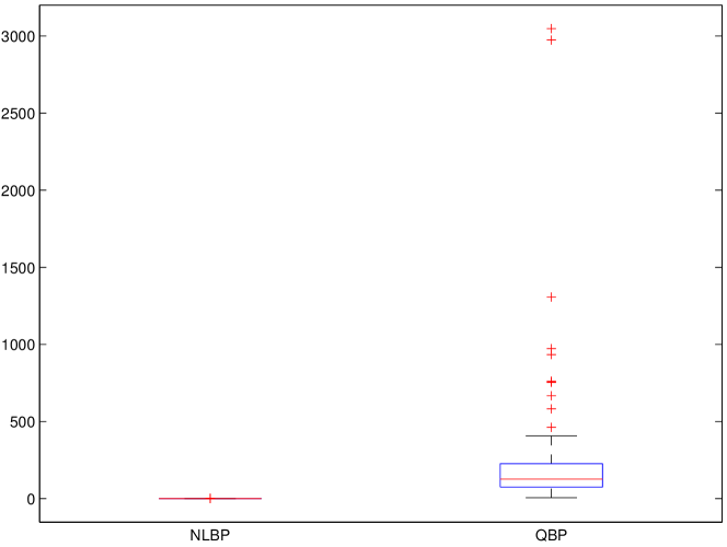
Figure 1: Box plot comparing NLBP and QBP for finding the dense solution of polynomial equation systems. The box plot summarizes the result from 100 trials.

VII Conclusion and Future Work

The main contribution of this paper is a nonlinear compressive sensing algorithms based on convex relaxations. The algorithm, referred to as nonlinear basis pursuit, is rather general in that it applies to any analytic nonlinearity by approximate it by a Taylor expansion of desired order. Nonlinear basis pursuit inherits theoretical guarantees, such as guaranteed recovery etc from its linear relative (basis pursuit) and therefore comes with theoretical guarantees that greedy algorithms often lack. Nonlinear basis pursuit takes the form of a convex non-smooth SDP which can be solved using conventional software for problems of interest.

It should be noticed that solving a nonlinear equation system is by itself a difficult problem. It is therefore quiet remarkable that we with rather high succes rate manage to find the sparsest solution to the nonlinear equation system. In addition, solving an overdetermined nonlinear equation system is also difficult. As shown in the example section, nonlinear basis pursuit not only find sparse solutions but also can also provide dense solutions to nonlinear equation system when no sparse solutions is available.

Convexifying nonlinear contraints using SDPs via its Taylor expansion is up to our knowledge novel and should find applications in many areas. This is seen as future research. Last, we have not discussed noise in this paper. However, this extension is trivial and a nonlinear extension of basis pursuit denoising follows.

VIII ACKNOWLEDGMENTS

The authors would like to acknowledge useful discussions and inputs from Yonina C. Eldar, Laura Waller, Filipe Maia, Stefano Marchesini and Michael Lustig.

References

- [1] A. Beck and Y. C. Eldar. Sparsity constrained nonlinear optimization: Optimality conditions and algorithms. Technical Report arXiv:1203.4580, Technion, 2012.
- [2] D. P. Bertsekas. Nonlinear Programming. Athena Scientific, 1999.
- [3] D. P. Bertsekas and J. N. Tsitsiklis. Parallel and Distributed Computation: Numerical Methods. Athena Scientific, 1997.
- [4] T. Blumensath. Compressed sensing with nonlinear observations and related nonlinear optimization problems. Technical Report arXiv:1205.1650, University of Oxford, 2012.
- [5] T. Blumensath and M. Davies. Gradient pursuit for non-linear sparse signal modelling. In European Signal Processing Conference, 2008.
- [6] S. Boyd, N. Parikh, E. Chu, B. Peleato, and J. Eckstein. Distributed optimization and statistical learning via the alternating direction method of multipliers. Foundations and Trends in Machine Learning, 2011.
- [7] A. Bruckstein, D. Donoho, and M. Elad. From sparse solutions of systems of equations to sparse modeling of signals and images. SIAM Review, 51(1):34–81, 2009.
- [8] E. Candès. Compressive sampling. In Proceedings of the International Congress of Mathematicians, volume 3, pages 1433–1452, Madrid, Spain, 2006.
- [9] E. Candès, Y. Eldar, T. Strohmer, and V. Voroninski. Phase retrieval via matrix completion. Technical Report arXiv:1109.0573, Stanford University, September 2011.
- [10] E. Candès, X. Li, Y. Ma, and J. Wright. Robust Principal Component Analysis? Journal of the ACM, 58(3), 2011.
- [11] E. Candès, T. Strohmer, and V. Voroninski. PhaseLift: Exact and stable signal recovery from magnitude measurements via convex programming. Technical Report arXiv:1109.4499, Stanford University, September 2011.
- [12] A. Chai, M. Moscoso, and G. Papanicolaou. Array imaging using intensity-only measurements. Technical report, Stanford University, 2010.
- [13] S. Chen, D. Donoho, and M. Saunders. Atomic decomposition by basis pursuit. SIAM Journal on Scientific Computing, 20(1):33–61, 1998.
- [14] W. Dai and O. Milenkovic. Subspace pursuit for compressive sensing signal reconstruction. IEEE Transactions on Information Theory, 55:2230–2249, 2009.
- [15] G. Davis, S. Mallat, and M. Avellaneda. Adaptive greedy approximations. Journal of Constructive Approximations, 13:57–98, 1997.
- [16] D. Donoho and M. Elad. Optimally sparse representation in general (nonorthogonal) dictionaries via -minimization. PNAS, 100(5):2197–2202, March 2003.
- [17] Y. C. Eldar and G. Kutyniok. Compresed Sensing: Theory and Applications. Cambridge University Press, 2012.
- [18] M. Fazel, H. Hindi, and S. P. Boyd. A rank minimization heuristic with application to minimum order system approximation. In Proceedings of the 2001 American Control Conference, pages 4734–4739, 2001.
- [19] M. X. Goemans and D. P. Williamson. Improved approximation algorithms for maximum cut and satisfiability problems using semidefinite programming. J. ACM, 42(6):1115–1145, November 1995.
- [20] M. Grant and S. Boyd. CVX: Matlab software for disciplined convex programming, version 1.21. http://cvxr.com/cvx, August 2010.
- [21] K. Jaganathan, S. Oymak, and B. Hassibi. Recovery of Sparse 1-D Signals from the Magnitudes of their Fourier Transform. ArXiv e-prints, June 2012.
- [22] H. Konno, J. Gotoh, T. Uno, and A. Yuki. A cutting plane algorithm for semi-definite programming problems with applications to failure discriminant analysis. Journal of Computational and Applied Mathematics, 146(1):141–154, 2002.
- [23] L. Li and B. Jafarpour. An iteratively reweighted algorithm for sparse reconstruction of subsurface flow properties from nonlinear dynamic data. Technical Report arXiv:0911.2270, University of Southern California, 2009.
- [24] I. Loris. On the performance of algorithms for the minimization of -penalized functionals. Inverse Problems, 25:1–16, 2009.
- [25] L. Lovász and A. Schrijver. Cones of matrices and set-functions and 0-1 optimization. SIAM Journal on Optimization, 1:166–190, 1991.
- [26] S. Marchesini. Ab Initio Undersampled Phase Retrieval. Microscopy and Microanalysis, 15, July 2009.
- [27] M. Moravec, J. Romberg, and R. Baraniuk. Compressive phase retrieval. In SPIE International Symposium on Optical Science and Technology, 2007.
- [28] D. Needell and J. Tropp. CoSaMP: Iterative signal recovery from incomplete and inaccurate samples. Appl. Comp. Harmonic Anal., 26:301–321, 2008.
- [29] Y. Nesterov. Semidefinite relaxation and nonconvex quadratic optimization. Optimization Methods & Software, 9:141–160, 1998.
- [30] H. Ohlsson, A. Yang, R. Dong, and S. S. Sastry. CPRL — an extension of compressive sensing to the phase retrieval problem. In P. Bartlett, F.C.N. Pereira, C.J.C. Burges, L. Bottou, and K.Q. Weinberger, editors, Advances in Neural Information Processing Systems 25, pages 1376–1384. 2012.
- [31] H. Ohlsson, A. Y. Yang, R. Dong, and S. Sastry. Compressive Phase Retrieval From Squared Output Measurements Via Semidefinite Programming. Technical Report arXiv:1111.6323, University of California, Berkeley, November 2011.
- [32] H. Ohlsson, A. Y. Yang, R. Dong, M. Verhaegen, and S. Sastry. Quadratic basis pursuit. Technical Report arXiv:1301.7002, University of California, Berkeley, 2013.
- [33] E. Osherovich, Y. Shechtman, A. Szameit, P. Sidorenko, E. Bullkich, S. Gazit, S. Shoham, E. B. Kley, M. Zibulevsky, I. Yavneh, Y. C. Eldar, O. Cohen, and M. Segev. Sparsity-based single-shot subwavelength coherent diffractive imaging. CLEO: Science and Innovations, 2012. CF3C.7.
- [34] P. Schniter and S. Rangan. Compressive phase retrieval via generalized approximate message passing. In Proceedings of Allerton Conference on Communication, Control, and Computing, Monticello, IL, USA, October 2012.
- [35] Y. Shechtman, A. Beck, and Y. C. Eldar. GESPAR: Efficient Phase Retrieval of Sparse Signals. ArXiv e-prints, January 2013.
- [36] Y. Shechtman, Y. C. Eldar, A. Szameit, and M. Segev. Sparsity based sub-wavelength imaging with partially incoherent light via quadratic compressed sensing. Opt. Express, 19(16):14807–14822, Aug 2011.
- [37] N.Z. Shor. Quadratic optimization problems. Soviet Journal of Computer and Systems Sciences, 25:1–11, 1987.
- [38] A. Szameit, Y. Shechtman, E. Osherovich, E. Bullkich, P. Sidorenko, H. Dana, S. Steiner, E. B. Kley, S. Gazit, T. Cohen-Hyams, S. Shoham, M. Zibulevsky, I. Yavneh, Y. C. Eldar, O. Cohen, and M. Segev. Sparsity-based single-shot subwavelength coherent diffractive imaging. Nature Materials, 11(5):455–459, May 2012.
- [39] A. Yang, A. Ganesh, Z. Zhou, S. Sastry, and Y. Ma. Fast -minimization algorithms for robust face recognition. Technical Report arXiv:1007.3753, University of California, Berkeley, 2012.