High-frequency homogenization of zero frequency stop band photonic and phononic crystals

Abstract

We present an accurate methodology for representing the physics of waves, for periodic structures, through effective properties for a replacement bulk medium: This is valid even for media with zero frequency stop-bands and where high frequency phenomena dominate.

Since the work of Lord Rayleigh in 1892, low frequency (or quasi-static) behaviour has been neatly encapsulated in effective anisotropic media; the various parameters come from asymptotic analysis relying upon the ratio of the array pitch to the wavelength being sufficiently small. However such classical homogenization theories break down in the high-frequency, or stop band, regime whereby the wavelength to pitch ratio is of order one. Furthermore, arrays of inclusions with Dirichlet data lead to a zero frequency stop band, with the salient consequence that classical homogenization is invalid.

Higher frequency phenomena are of significant importance in photonics (transverse magnetic waves propagating in infinite conducting parallel fibers), phononics (anti-plane shear waves propagating in isotropic elastic materials with inclusions), and platonics (flexural waves propagating in thin-elastic plates with holes). Fortunately, the recently proposed high-frequency homogenization (HFH) theory is only constrained by the knowledge of standing waves in order to asymptotically reconstruct dispersion curves and associated Floquet-Bloch eigenfields: It is capable of accurately representing zero-frequency stop band structures. The homogenized equations are partial differential equations with a dispersive anisotropic homogenized tensor that characterizes the effective medium.

We apply HFH to metamaterials, exploiting the subtle features of Bloch dispersion curves such as Dirac-like cones, as well as zero and negative group velocity near stop bands in order to achieve exciting physical phenomena such as cloaking, lensing and endoscope effects. These are simulated numerically using finite elements and compared to predictions from HFH. An extension of HFH to periodic supercells enabling complete reconstruction of dispersion curves through an unfolding technique is also introduced.

1 Introduction

Over the past 25 years, many significant advances have created a deep understanding of the optical properties of photonic crystals (PCs) [yablonovitch87a, john87a]; such periodic structures prohibit the propagation of light, or allow it only in certain directions at certain frequencies, or localize light in specified areas. This sort of metamaterial (using the consensual terminology for artificial materials engineered to have desired properties that may not be found in nature, such as negative refraction, see e.g. [smith04a, sar_rpp05]) enables a marked enhancement of control over light propagation; this arises from, for instance, the periodic patterning of small metallic inclusions embedded within a dielectric matrix [pendry96a, nicorovici95a]. PCs are periodic devices whose spectrum is characterized by photonic band gaps and pass bands, just as electronic band gaps exist in semiconductors: In PCs, light propagation is disallowed for certain frequencies in certain directions. This effect is well known [joannopoulos08a, zolla05a] and forms the basis of many devices, including Bragg mirrors, dielectric Fabry-Perot filters, and distributed feedback lasers; all of these contain low-loss dielectrics periodic in one dimension, so are one-dimensional PCs. Such mirrors are tremendously useful, but their reflecting properties critically depend upon the frequency of the incident wave in regard with its incidence [markos08a]. For broad frequency ranges, one wishes to reflect light of any polarization at any angle (which requires a complete photonic band gap) and for Dirichlet media (i.e. those composed with microstructure where the field is zero on the microparticles) such a gap occurs at zero-frequency. It is therefore possible to create seismic shields for low-frequency waves [brule13a, antonakakis13b]. Extending these ideas to higher dimensions allows for a much greater range of optical effects: all-angle negative refraction [luo02a, zengerle87a], ultra-refraction [farhat10b, craster11a] and cloaking at Dirac-like cones [chan12a]: We will demonstrate here that an effective medium can be created that reproduces these effects.

The considerable recent activity in this area is, in part, fuelled by advances in numerical techniques, based on Fourier expansions in the vector electromagnetic Maxwell equations [joannopoulos08a], Finite Elements [zolla05a] and Multipole and lattice sums [movchan02a] for cylinders, to name but a few, that allow one to visualize the various effects and design PCs. The multipole method takes its root in a seminal paper of Lord Rayleigh [rayleigh92a] which is the foundation stone upon which the current edifice of homogenization theories is built. More precisely, in that paper, John William Strutt, the third Lord Rayleigh, solved Laplace’s equation in two dimensions for rectangular arrays of cylinders, and in three dimensions for cubic lattices of spheres. However, a limitation of Rayleigh’s algorithm is that it does not hold when the volume fraction of inclusions increases. Multipole methods, in conjunction with lattice sums, overcome such obstacles and lead to the Rayleigh system which is an infinite linear algebraic system; this formulation, in terms of an eigenvalue problem, facilitates the construction of dispersion curves and the study of both photonic and phononic band-gap structures. In the limit of small inclusion radii, when propagating modes are very close to plane waves, one can truncate the Rayleigh system ignoring the effect of higher multipoles, to produce a series of approximations each successively more accurate to higher values of filling fraction. At the dipole order, one is able to fit the acoustic band, which has a linear behaviour in the neighbourhood of zero frequency, except of course in the singular case whereby Dirichlet data is enforced on the boundary inclusions [poulton01a] and there is a zero frequency stop-band: This is a substantial limitation of this truncation. We will derive here the exact solution for zero radius Dirichlet holes, avoiding multipole expansions, and show dispersion curves whose features lead to interesting topical effects, such as Dirac-like cone cloaking and degenerate points [chan12a] which emerge very naturally in this exact solution.

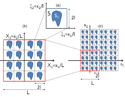
Figure 1: High Frequency Homogenization (HFH) principle: An elementary cell (a) of sidelength $2l$, modelled by a fast oscillating variable ${\bm{\xi}}$, is repeated periodically within a supercell (b) of sidelength $L$, modelled by a slow variable ${\bf X}$, which is itself repeated periodically in space (c). One then assumes that the parameter $\epsilon=l/L$ is small, and its vanishing limit thereafter studied. The leading order, homogenized, term of Floquet-Bloch eigenfields within the crystal are then sought as $u_{0}({\bf X},{\bm{\xi}})=f_{0}({\bf X})U_{0}({\bm{\xi}};\Omega_{0})$, wherein $f_{0}$ accounts for variations of the fields on the order of the supercells, and $U_{0}$ captures their fast oscillations in the much smaller cells, when either periodic or anti-periodic conditions are enforced on the cells: Perturbing away from these standing waves of frequency $\Omega_{0}$ allows for a complete reconstruction of the Bloch spectrum and associated Floquet-Bloch eigenfields.

Although the numerical approaches discussed briefly are efficient they still do require substantial computational effort and can obscure physical understanding and interpretation. Here we substantially reduce the numerical complexity of the wave problem using asymptotic analysis; this has been developed over the past 35 years by applied mathematicians primarily for solving partial differential equations, with rapidly oscillating periodic coefficients, in the context of thermostatics, continuum mechanics or electrostatics [bensoussan78a, jikov94a, milton02a]. The available literature on such effective medium theories is vast, but it seems that only a very few groups have addressed such problems as the homogenization of media, with moderate contrast in the material properties, in three-dimensions [zolla00a, wellander03] and high-contrast two-dimensional [zhikov00a, bouchitte04a, cherednichenko06a] photonic crystals, that have important potential applications in photonics. Besides this, the aforementioned literature does not address the challenging problem of homogenization for moderate contrast photonic crystals near stop band frequencies: Classical homogenization is constrained to low frequencies and long waves in moderate contrast PCs [silveirinha05a] and so-called high-contrast homogenization only captures the essence of stop bands in PCs when the permittivity inside the inclusions is much higher than that of the surrounding matrix (the contrast being typically on the order to $\epsilon^{-2}$ where $\epsilon$ is the array pitch which in turn is much smaller than the wavelength). This latter area of homogenization theory is fuelled by interest in artificial magnetism, initiated by the work of O’Brien and Pendry [obrien02a]. However, moderate contrast one-dimensional photonic crystals have been recently shown to display not only artificial magnetism, but also chirality [yan2013a], which is an onset to negative refraction [pendry04b] .

For all these reasons, there is a strong demand for high-frequency homogenization theories of PCs in order to grasp, and fully exploit, the rich behaviour of photonic band gap structures [notomi00, paul11]. This has created a suite of extended homogenization theories for periodic media called Bloch homogenisation [conca95a, allaire05a, birman06a, hoefer11a]. There is also a flourishing literature on developing homogenized elastic media, with frequency dependent effective parameters, also based upon periodic media [nematnasser11a]: There is considerable interest in creating effective continuum models of microstructured media that break free from the conventional low frequency homogenisation limitations.

In this paper, we apply the HFH theory proposed by one of us three years ago [craster10a] to the physics of zero frequency band gap structures, not only in the context of photonics, but also phononics for anti-plane shear waves in periodic arrays of inclusions, and platonics with flexural waves in pinned plates. The latter analysis is made possible thanks to the extension of HFH to plate theory, developed by two of us two years ago [antonakakis12a]. Our aim is to show the universal features of stop band structures thanks to HFH, and to further exemplify their potential use in control of light and mechanical waves, with novel applications ranging from cloaking [milton06a, guenneau07b] to anti-earthquake seismic shields [antonakakis13a, brule13a].

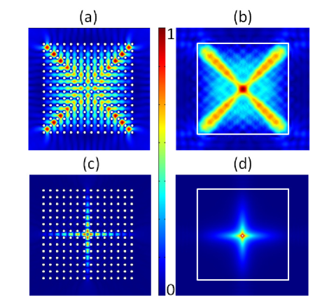
Figure 2: Dynamic effective anisotropy: A time-harmonic source located inside a square array of pitch 2 consisting of 196 circular constrained holes of radius 0.4 leads to a wave pattern resembling a Saint-Andrews’ cross at frequency $\Omega=1.966$ (a) FEM (b) HFH, and a Saint-George’s cross at frequency $\Omega=2.75$ (c) FEM (d) HFH.

We show in Fig. 1 what HFH does in practice: It focuses its attention on the physics within a supercell of sidelength $L$, which is the long- scale, and further captures the fine features of field’s oscillations inside an elementary cell of sidelength $2l$ much smaller than $L$ [craster10a]. The wavelength need not be large compared to $l$ in order to perform the asymptotic analysis, as the small parameter $\epsilon=l/L$ only requires the supercell to be much larger than its constituent elementary cells; this contrasts with classical homogenization that assumes the cells are much smaller than the wavelength. In this way, one replaces a periodic structure by a homogenized one, on the long-scale, at any frequency and classical homogenization is just a particular case of HFH [antonakakis13a]. An illustration of the HFH theory is in Fig. 2; the left panels are from full finite element simulations of an array of cylindrical holes (infinite conducting boundary conditions of the holes which are for transverse magnetic (TM) waves in electromagnetism, or clamped shear horizontal waves in elasticity) excited at the array centre by a line source and the right panels replace the array with its effective HFH medium which reproduces the large scale behaviour. For the frequencies chosen, two very distinct cross-shaped propagations, a Saint Andrews’ cross (or saltire) Fig. 2(a),(b), and a Saint George’s cross Fig. 2 (c),(d) are achieved; these distinctive shapes are created by excitations at precise frequencies that are identified from the dispersion curves, [craster12b], this strong frequency dependent anisotropy is a recurrent feature of PCs. One sees that the HFH neatly reproduces in Fig. 2(b,d) the fine features of the full finite element simulations. Interpretation is provided by using the Brillouin zone of Fig. 3 and dispersion curves shown in Fig. 4. The square array of holes behaves as two dramatically contrasting effective media at frequency $\Omega=1.966$, see Fig. 2(a,b), which stands on the edge of the zero-frequency stop band that coincides with the lower edge of the second stop band; and at frequency $\Omega=2.75$ which stands on the upper edge of the second stop band, wherein the dispersion curve is nearly flat is the $MX$ direction; both these frequencies are well beyond the range of applicability of classical homogenization.

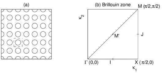
Figure 3: Panel (a) shows a square array of circular cylinders, with the elementary cell as the dashed box. In (b) the irreducible Brillouin zone is shown together with lettering necessary for our discussion of folding in section 4.1.2.

Our aim is to generate HFH for arrays of holes with Dirichlet conditions, so this is for TM waves in electromagnetism, and then compare through full numerical simulations of HFH and finite elements to show how the behaviour of the numerous interesting optical effects emerge naturally through the coefficients of our effective medium. This is intertwined with a knowledge and understanding of the wave structure for a perfect medium where the dispersion relations connecting the phase shift across an elementary cell with the frequency is key. In section 2 we set up the mathematical framework leading to the effective medium equation (15), this is in a non-dimensional setting so for clarity in section 3 the main results are summarized in a dimensional setting. There are degenerate cases that are of substantial interest and connect with Dirac-like dispersion [chan12a] and these lead to a different effective equation also outlined in section 3.

A first step in verifying the HFH theory is by asymptotically reproducing the dispersion curves for perfect infinite arrays, and we use both circular and square holes for illustration, as shown in section 4. Local to the edges of the Brillouin zone there are standing wave frequencies and the local asymptotic behaviour is given from the effective medium equation. Importantly, one can then predict apriori, from the signs of the HFH coefficients with the effective equation, how the bulk medium will behave. As a further illustration, holes that degenerate to a point are treated (section 4.3) as there is then an exact and simple solution for the dispersion relation, furthermore in this case degeneracies occur. Finally, in section 5 we compare HFH with full numerical simulations showing the full range of features available and how HFH represents them. Some concluding remarks are drawn together in section 6.

2 General theory

A two dimensional structure composed of a doubly periodic, i.e. periodic in both $x$ and $y$ directions, square array of cells with, not necessarily circular, identical holes inside them is considered (see Fig. 3). We are primarily concerned with electromagnetism where Maxwell’s equations separate into transverse electric (TE) and TM polarizations and the natural boundary conditions on the holes are then Neumann and Dirichlet respectively; the asymptotics for the former are considered in [antonakakis13a] and applications in metamaterials are illustrated with split ring resonators [pendry99a]. In the current article our emphasis is rather different, and is upon TM polarization for which the Dirichlet conditions induce different effects, such as zero-frequency stop bands, and require a modified theory.

Assuming an $\exp(-i\omega t)$ time dependence that is considered understood, and henceforth suppressed, the governing equation is,

$$\nabla_{{\bf x}}\cdot[\hat{a}({\bm{\xi}})\nabla_{{\bf x}}u({\bf x})]+\omega^{2}\hat{\rho}({\bm{\xi}})u({\bf x})=0$$ (1)

on $-\infty<x_{1},x_{2}<\infty$ where $\omega$ is the angular frequency. In the periodic setting, each cell is identical and the material is characterized by two periodic functions on the short-scale, in ${\bm{\xi}}\equiv(x_{1}/l,x_{2}/l)$, namely $\hat{a}({\bm{\xi}})$ and $\hat{\rho}({\bm{\xi}})$. In the context of photonics, these are the inverse of permeability ($\mu^{-1}$), and permittivity ($\varepsilon$), respectively, which are related to the wavespeed of light in vacuum $c$ via the refractive index $n$ as follows: $\varepsilon\mu=n^{2}c^{-2}$. The unknown $u$ physically is the longitudinal component $E_{z}$ of the out-of-plane electric field ${\bf E}=(0,0,E_{z})$, bearing in mind that the transverse magnetic field ${\bf H}=(H_{x},H_{y},0)$ is retrieved from Maxwell’s equation ${\bf H}=i\omega^{-1}\mu^{-1}\nabla\times{\bf E}$. In the context of phononics, $\hat{a}({\bm{\xi}})$ and $\hat{\rho}({\bm{\xi}})$ would stand respectively for the shear modulus and the density of an isotropic elastic medium, and the unknown $u$ would correspond to the out-of-plane displacement (amplitude of SH shear waves). One can also easily draw analogies with acoustic pressure waves in a fluid, or linear surface water waves, which explains the activity related to finding correspondences between models of electromagnetic [sar_rpp05] and acoustic [craster12a] metamaterials. The length of the direct lattice base vectors are taken equal and to be $2l$, and define a short lengthscale. The overall dimension of the structure is of a much longer length-scale, $L$; the ratio of scales, $\epsilon\equiv l/L\ll 1$ then provides a small parameter for use later in the asymptotic scheme.

A non-dimensionalization of the physical functions by setting, $\hat{a}\equiv\hat{a}_{0}a({\bm{\xi}})$ and $\hat{\rho}\equiv\hat{\rho}_{0}\rho({\bm{\xi}})$ is convenient. Equation (1) then becomes

$$l^{2}\nabla_{{\bf x}}\cdot[a({\bm{\xi}})\nabla_{{\bf x}}u({\bf x})]+\Omega^{2}\rho({\bm{\xi}})u({\bf x})=0\quad{\rm with}\quad\Omega=\frac{\omega l}{\hat{c}_{0}}$$ (2)

as the non-dimensional frequency and $\hat{c}_{0}=\sqrt{\hat{a}_{0}/\hat{\rho}_{0}}$. The two scales, $l,L$, then motivate two new coordinates namely ${\bf X}={\bf x}/L$, and ${\bm{\xi}}={\bf x}/l$ that are treated as independent, and placing this change of coordinates into (2) we obtain,

$$\nabla_{{\bm{\xi}}}\cdot[a({\bm{\xi}})\nabla_{{\bm{\xi}}}u({\bf X},{\bm{\xi}})]+\Omega^{2}\rho({\bm{\xi}})u({\bf X},{\bm{\xi}})$$

$$\qquad+\epsilon[2a({\bm{\xi}})\nabla_{\bm{\xi}}+\nabla_{{\bm{\xi}}}a({\bm{\xi}})]\cdot\nabla_{{\bf X}}u({\bf X},{\bm{\xi}})+\epsilon^{2}a({\bm{\xi}})\nabla^{2}_{\bf X}u({\bf X},{\bm{\xi}})=0.$$ (3)

For wave propagation through a perfect lattice there exist standing waves at specific eigenfrequencies, $\Omega_{0}$, and their eigenmodes satisfy periodic, or anti-periodic (out-of-phase) boundary conditions on the edges of the cell: We obtain asymptotic solutions based upon these standing waves.

A key point, from this separation of scales, is that the boundary conditions on the short-scale are known. For instance, periodic conditions in ${\bm{\xi}}$ on the edges of the cell are

$$u|_{\xi_{i}=1}=u|_{\xi_{i}=-1}\quad{\rm and}\quad u_{,\xi_{i}}|_{\xi_{i}=1}=u_{,\xi_{i}}|_{\xi_{i}=-1}$$ (4)

where $u_{,\xi_{i}}$ denotes partial differentiation with respect to $\xi_{i}$. An almost identical analysis holds near the anti-periodic standing wave frequencies: We illustrate the periodic case for definiteness. On the long-scale we set no boundary conditions, and indeed the methodology we present can be used even when the problem is not perfectly periodic [craster11a].

The following ansatz is taken

$$u({\bf X},{\bm{\xi}})=u_{0}({\bf X},{\bm{\xi}})+\epsilon u_{1}({\bf X},{\bm{\xi}})+\epsilon^{2}u_{2}({\bf X},{\bm{\xi}})+\ldots,\quad\Omega^{2}=\Omega_{0}^{2}+\epsilon\Omega_{1}^{2}+\epsilon^{2}\Omega_{2}^{2}+\ldots:$$ (5)

Since $u({\bf X},{\bm{\xi}})$ is periodic in ${\bm{\xi}}$ so are the $u_{i}({\bf X},{\bm{\xi}})$’s. This leads to a hierarchy of equations in increasing powers of $\epsilon$: The leading order followed by the first order, second order and so on. The first three equations in ascending order yield

$$(au_{0,\xi_{i}})_{,\xi_{i}}+\Omega_{0}^{2}\rho u_{0}=0$$ (6)

$$(au_{1,\xi_{i}})_{,\xi_{i}}+\Omega_{0}^{2}\rho u_{1}=-(2au_{0,\xi_{i}}+a_{,\xi_{i}}u_{0})_{,X_{i}}-\Omega_{1}^{2}\rho u_{0}$$ (7)

$$(au_{2,\xi_{i}})_{,\xi_{i}}+\Omega_{0}^{2}\rho u_{2}$$

$$\qquad=-au_{0,X_{i}X_{i}}-(2au_{1,\xi_{i}}+a_{,\xi_{i}}u_{1})_{,X_{i}}-\Omega_{1}^{2}\rho u_{1}-\Omega_{2}^{2}\rho u_{0}.$$ (8)

We start by expressing a solution for the leading order equation. For a specific eigenvalue $\Omega_{0}$ there is a corresponding eigenmode $U_{0}({\bm{\xi}};\Omega_{0})$, periodic in ${\bm{\xi}}$, and the leading order solution is

$$u_{0}({\bf X},{\bm{\xi}})=f_{0}({\bf X})U_{0}({\bm{\xi}};\Omega_{0}).$$ (9)

The function $f_{0}({\bf X})$ is determined later on, indeed the whole point is to deduce a long-scale continuum partial differential equation for $f_{0}$ entirely upon the long-scale. We begin with a treatment of isolated eigenvalues, however repeated eigenvalues also arise, and require modifications, and will be dealt with in sections 2.2 and 2.3: These are relevant to Dirac-like cones [chan12a].

Dirichlet conditions on the inside boundary of the cell, $\partial S_{2}$, where $S$ denotes the surface of the cell in the ${\bm{\xi}}$ coordinates, yield

$$u({\bf X},{\bm{\xi}})|_{\partial S_{2}}=0\iff u_{i}({\bf X},{\bm{\xi}})|_{\partial S_{2}}=0,\quad i\in\ \mathbb{N}$$ (10)

and are set in the short-scale ${\bm{\xi}}$ so, for $i=0$, $U_{0}({\bm{\xi}};\Omega_{0})|_{\partial S_{2}}=0$.

To deduce the long-scale PDE for $f_{0}({\bf X})$ we follow [craster10a], making changes where necessary due to the change in boundary conditions. Equation (7) is multiplied by $U_{0}$ and integrated over the cell’s surface to obtain

$$\int\int_{S}\left(U_{0}(au_{1,\xi_{i}})_{,\xi_{i}}+\Omega_{0}^{2}\rho U_{0}u_{1}\right)dS$$

$$\qquad\qquad=-f_{0,X_{i}}\int\int_{S}(aU_{0}^{2})_{,\xi_{i}}dS-f_{0}\Omega_{1}^{2}\int\int_{S}\rho U_{0}^{2}dS.$$ (11)

The first integral of the right hand side is converted to a path integral along $\partial S$ using a corollary of the divergence theorem. The periodic conditions on $\partial S_{1}$ and the homogeneous Dirichlet conditions of $U_{0}$ on $\partial S_{2}$ make it vanish. We continue by subtracting the integral over the cell of the product of equation (6) with $u_{1}/f_{0}$ to obtain

$$\int\int_{S}(U_{0}(au_{1,\xi_{i}})_{,\xi_{i}}-u_{1}(aU_{0,\xi_{i}})_{,\xi_{i}})dS=-f_{0}\Omega_{1}^{2}\int\int_{S}\rho({\bm{\xi}})U_{0}^{2}dS.$$ (12)

Using Green’s theorem equation (12) becomes

$$\int_{\partial S}a({\bm{\xi}})\left(U_{0}\frac{\partial u_{1}}{\partial n}-u_{1}\frac{\partial U_{0}}{\partial n}\right)ds=-f_{0}\Omega_{1}^{2}\int\int_{S}\rho({\bm{\xi}})U_{0}^{2}dS$$ (13)

where $\partial S=\partial S_{1}+\partial S_{2}$. Due to periodic (or anti-periodic) boundary conditions of $u$ and its first derivatives with respect to $\xi_{i}$ on $\partial S_{1}$, and due to the homogeneous Dirichlet boundary conditions of the $u_{i}$’s on $\partial S_{2}$, the left hand side of equation (13) vanishes. It follows that $\Omega_{1}=0$, which is an important deduction as it implies that the asymptotic behaviour of dispersion curves near isolated eigenfrequencies is at least quadratic. We then solve for $u_{1}({\bf X},{\bm{\xi}})$ and obtain

$$u_{1}({\bf X},{\bm{\xi}})=f_{1}({\bf X})U_{0}({\bm{\xi}};\Omega_{0})+\nabla_{\bf X}f_{0}({\bf X})\cdot{\bf U_{1}}({\bm{\xi}}).$$ (14)

The first term is simply a homogeneous solution that is irrelevant, and the vector function ${\bf U}_{1}$ is a particular solution. Quite often exact solutions for $u_{1}$ or ${\bf U}_{1}$ are not possible to obtain so one must use numerical solutions and this is described in section 5. We now move to the second order equation to compute $f_{0}({\bf X})$ and $\Omega_{2}^{2}$. Similarly to the first order equation, we multiply equation (8) by $U_{0}$ then subtract the product of equation (7) with $u_{2}/f_{0}$, finally we integrate over the cell’s surface to obtain the following effective equation for $f_{0}$

$$T_{ij}f_{0,X_{i}X_{j}}+\Omega_{2}^{2}f_{0}=0,\quad{\rm with}\quad T_{ij}=\frac{t_{ij}}{\int\int_{S}\rho U_{0}^{2}dS}\quad{\rm for}\quad i,j=1,2,$$ (15)

which is the main result of this article. In particular, the coefficients $T_{ij}$ encode the anisotropy at a specific frequency and the $t_{ij}$’s are integrals over the small-scale cell

$$t_{ii}=\int\int_{S}aU_{0}^{2}dS+2\int\int_{S}aU_{1_{i},\xi_{i}}U_{0}dS+\int\int_{S}a_{,\xi_{i}}U_{1_{i}}U_{0}dS,$$ (16)

$$t_{ij}=2\int\int_{S}aU_{1_{j},\xi_{i}}U_{0}dS+\int\int_{S}a_{,\xi_{i}}U_{1_{j}}U_{0}dS\quad{\rm for}\quad i\neq j,$$ (17)

where $U_{1_{i}}$ is the ith component of vector function ${\bf U}_{1}$. Note that there is no summation over repeated indexes for $t_{ii}$. The PDE for $f_{0}$, equation (15), is crucial as the local microstructure is completely encapsulated within the tensor $T_{ij}$; these are, for a specific structure at an $\Omega_{0}$, just numerical values as illustrated in table 2. Notably the tensor can have negative values, or components, and it allows one to interpret and, even more importantly, predict changes in behaviour or when specific effects occur. The structure of the tensor depends upon the boundary conditions of the holes, the results here, for instance, are different from those of the Neumann case [antonakakis13a]. Another key point is that numerically the short scale is no longer present and the PDE (15) is simple and quick to solve numerically, or even by hand.

One primary aim of the present article is to deduce formulae for the local behaviour of dispersion curves near standing wave frequencies as these shed light upon the physical effects observed. For this one returns to the perfect lattice and then Floquet Bloch boundary conditions on the elementary cell lead immediately to $f_{0}({\bf X})=\exp(i\kappa_{j}X_{j}/\epsilon)$. In this notation $\kappa_{j}=K_{j}-d_{j}$ and $d_{j}=0,\pi/2,-\pi/2$ depending on the location in the Brillouin zone. Equation (15) gives

$$\Omega\sim\Omega_{0}+\frac{T_{ij}}{2\Omega_{0}}\kappa_{i}\kappa_{j}$$ (18)

and these locally quadratic dispersion curves are completely described by $\Omega_{0}$ and the tensor $T_{ij}$.

2.1 Classical singularly perturbed zero-frequency limit

It is natural, at this point, to contrast with usual homogenization theories. As is well-known [nicorovici95a, mcphedran97a] one cannot homogenize the TM polarized case because the conventional approach only works at low frequencies in a quasi-static limit. Some authors attribute this to a singular perturbation, or non-commuting limit, problem whereby letting first the Bloch wavenumber and then the frequency tend to zero, or doing it the way around, leads to a different result [poulton01a]. The approach used in this article overcomes this by releasing the theory from the low-frequency constraint. For TE polarization [antonakakis13a] one can explicitly connect the theories and show that the low frequency theory is a sub-set of the high frequency approach. The TM case differs fundamentally as there is a zero-frequency stop-band.

We now prove that the usual homogenization cannot give the asymptotic behaviour even at low-frequency. Setting $\Omega^{2}=\epsilon^{2}\Omega_{2}^{2}+\ldots$, that is, going to low frequency, and assuming that $u_{0}({\bf X},\bm{\xi})=f({\bf X})U_{0}({\bm{\xi}})$ is non-zero one arrives at a contradiction: At leading order $U_{0}(\bm{\xi})$ satisfies $\nabla^{2}U_{0}=0$ where for brevity we have set $a=1$, complemented by $U_{0}=0$ on the hole and periodic (anti-periodic) boundary condition on the edge of the cell. From the uniqueness properties of the Laplacian $U_{0}\equiv 0$ is the unique solution and hence usual homogenization cannot find the asymptotics at low frequency in this Dirichlet case.

2.2 Repeated eigenvalues: linear asymptotics

Repeated eigenvalues are commonplace in specific examples and, as we shall see, are particularly relevant to Dirac-like cones [chan12a] that have practical significance. If we assume repeated eigenvalues of multiplicity $p$ the general solution for the leading order problem becomes,

$$u_{0}=f_{0}^{(l)}({\bf X})U_{0}^{(l)}({\bm{\xi}};\Omega_{0})$$ (19)

where we sum over the repeated superscripts $(l)$. Proceeding as before, we multiply equation (7) by $U_{0}^{(m)}$, subtract $u_{1}((aU^{(m)}_{0,\xi_{i}})_{\xi_{i}}+\Omega_{0}^{2}\rho U_{0}^{(m)})$ then integrate over the cell to obtain,

$$f_{0,X_{i}}^{(l)}\int\int_{S}U_{0}^{(m)}(2aU_{0,\xi_{i}}^{(l)}+a_{\xi_{i}}U_{0}^{(l)})dS+\Omega_{1}^{2}f_{0}^{(l)}\int\int_{S}\rho U_{0}^{(l)}U_{0}^{(m)}dS=0.$$ (20)

There is now a system of coupled partial differential equations for the $f_{0}^{(l)}$ and, provided $\Omega_{1}\neq 0$, the leading order behaviour of the dispersion curves near the $\Omega_{0}$ is now linear (these then form Dirac-like cones). These coupled partial differential equations on the long-scale now replace (15) near these frequencies.

For the perfect lattice and Bloch wave problem, we set $f_{0}^{(l)}={\hat{f}}_{0}^{(l)}\exp(i\kappa_{j}X_{j}/\epsilon)$ and obtain the following equations,

$$\left(i\frac{\kappa_{j}}{\epsilon}{\bf A}_{jml}+\Omega_{1}^{2}{\bf B}_{ml}\right){\hat{f}}_{0}^{(l)}=0,\quad{\rm for}\quad m=1,2,...,p$$ (21)

where,

$${\bf A}_{jml}=\int\int_{S}U_{0}^{(m)}(2aU_{0,\xi_{j}}^{(l)}+a_{,\xi_{j}}U_{0}^{(l)})dS$$ (22)

and

$${\bf B}_{ml}=\int\int_{S}\rho U_{0}^{(l)}U_{0}^{(m)}dS.$$ (23)

The system of equations (21) is written simply as,

$${\bf C}{\hat{\bf F}}_{0}=0,$$ (24)

with ${\bf C}_{ll}=\Omega_{1}^{2}{\bf B}_{ll}$ and ${\bf C}_{ml}=i\kappa_{j}{\bf A}_{jml}/\epsilon$ for $l\neq m$. One must then solve for $\Omega_{1}^{2}=\pm\sqrt{\alpha_{ij}\kappa_{i}\kappa_{j}}/\epsilon$ when the determinant of ${\bf C}$ vanishes and the asymptotic relation is,

$$\Omega\sim\Omega_{0}\pm\frac{1}{2\Omega_{0}}\sqrt{\alpha_{ij}\kappa_{i}\kappa_{j}}.$$ (25)

If $\Omega_{1}$ is zero, one must go to the next order and a slightly different analysis ensues.

$\alpha_{11}$	$\alpha_{22}$	$\Omega_{0}$
$2\pi^{2}$	$2\pi^{2}$	$\pi$
$4\pi^{2}$	$4\pi^{2}$	$\sqrt{2}\pi$

Table 1: The coefficients $\alpha_{ii}$, necessary in equation (25) for the two Dirac-like cones at point $\Gamma$ of the Brillouin zone for a doubly periodic array of constrained points.

2.3 Repeated eigenvalues: Quadratic asymptotics

Assuming that $\Omega_{1}$ is zero, $u_{1}=f_{0,X_{k}}^{(l)}U_{1_{k}}^{(l)}$ (we again sum over all repeated $(l)$ superscripts) and advance to second order using (8). Taking the difference between the product of equation (8) with $U_{0}^{(m)}$ and $u_{2}((aU_{0,\xi_{i}})_{,\xi_{i}}+\Omega_{0}^{2}\rho U_{0})$ and then integrating over the elementary cell gives

$$f_{0,X_{i}X_{i}}^{(l)}\int\int_{S}aU_{0}^{(m)}U_{0}^{(l)}dS+f_{0,X_{k}X_{j}}^{(l)}\int\int_{S}U_{0}^{(m)}(2aU_{1_{k},\xi_{j}}^{(l)}+a_{,\xi_{j}}U_{1_{k}}^{(l)})dS$$

$$\quad+\Omega_{2}^{2}f_{0}^{(l)}\int\int_{S}\rho U_{0}^{(m)}U_{0}^{(l)}dS=0,\quad{\rm for}\quad m=1,2,...,p$$ (26)

as a system of coupled PDEs. The above equation is presented more neatly as

$$f_{0,X_{i}X_{i}}^{(l)}{\bf A}_{ml}+f_{0,X_{k}X_{j}}^{(l)}{\bf D}_{kjml}+\Omega_{2}^{2}f_{0}^{(l)}{\bf B}_{ml}=0,\quad{\rm for}\quad m=1,2,...,p.$$ (27)

For the Bloch wave setting, using $f_{0}^{(l)}({\bf X})={\hat{f}}_{0}^{(l)}\exp(i\kappa_{j}X_{j}/\epsilon)$ we obtain the following system,

$$\left(-\frac{\kappa_{i}\kappa_{i}}{\epsilon^{2}}{\bf A}_{ml}-\frac{\kappa_{k}\kappa_{j}}{\epsilon^{2}}{\bf D}_{kjml}+\Omega_{2}^{2}{\bf B}_{ml}\right){\hat{f}}_{0}^{(l)}=0,\quad{\rm for}\quad m=1,2,...,p$$ (28)

and this determines the asymptotic dispersion curves.

3 Effective dispersive media

The major goal of HFH is to represent the periodic medium of finite extent using an effective homogeneous medium and the main result of this article is in achieving this, and for clarity this is summarized in this section back in the dimensional setting.

Transforming equation (15) back to the original $x_{i}=X_{i}L$ coordinates and using the solution of $\Omega_{2}$ we obtain an effective medium equation for ${\hat{f}}_{0}$ that is,

$$T_{ij}{\hat{f}}_{0,x_{i}x_{j}}({\bf x})+\frac{\Omega^{2}-\Omega_{0}^{2}}{l^{2}}{\hat{f}}_{0}({\bf x})=0.$$ (29)

The nature of equation (29) is not necessarily elliptic since $T_{11}$ and $T_{22}$ can take different values and/or different signs. In the illustrations herein the $T_{ij}=0$ for $i\neq j$. The hyperbolic behaviour of equation (29) yields asymptotic solutions that describe the endoscope effects where, if one of the $T_{ii}$ coefficients is zero as often happens near the point $M$ of the Brillouin zone, waves propagate only in one direction. Note that when the cell has the adequate symmetries the dispersion relation near point $G(0,\pi/2)$ is identical to that near point $X(\pi/2,0)$ which explains the existence of two orthogonal directions of propagation instead of only one.

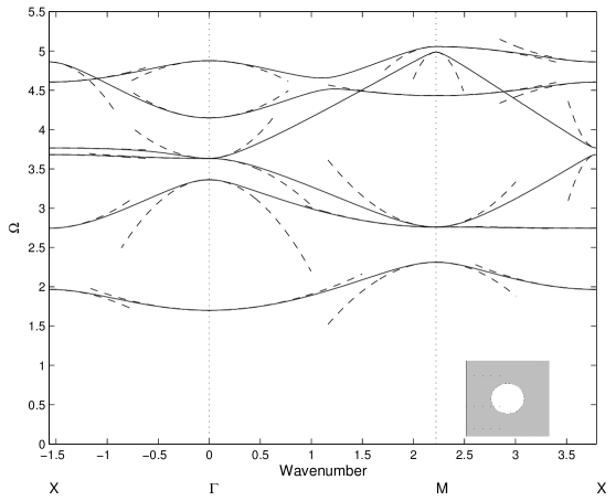
Figure 4: The dispersion diagram for a doubly periodic array of square cells with circular inclusions, of radius $0.4$, fixed at their inner boundaries shown for the irreducible Brillouin zone of Fig. 3. The dispersion curves are shown in solid lines and the asymptotic solutions from HFH are shown in dashed lines.

$T_{11}$	$T_{22}$	$\Omega_{0}$
$0.698841854976085$	$0.698841854976085$	$1.700916617638699$
$7.867675441589871$	$7.867675441589871$	$3.361627184739501$
$0.3230$	$-8.998$	$3.632730109763024$
$4.9681$	$14.2899$	$3.632730129014608$
$4.775527931399718$	$4.775527931399718$	$4.148661549527329$
$-4.279843054160115$	$-4.279843054160115$	$4.877003447953185$

Table 2: The first six standing wave frequencies for in-phase waves at $\Gamma$, cf. Fig. 4, together with associated values for $T_{11}$ and $T_{22}$. Symmetry between $T_{11}$ and $T_{22}$ is breaking when the multiplicity of the eigenvalue is greater than two. Negative group velocity is demonstrated by the negative sign of both $T_{ij}$’s.

At Dirac-like cones the linear behaviour of the effective medium yields an equation slightly different from (29). Regarding the zero radius holes, presented in the following section 4.3, it consists of a system of three coupled PDE’s that uncouple to yield one identical PDE for all $f_{0}^{(i)}$s that is of the form,

$${\hat{f}}_{0,x_{i}x_{i}}({\bf x})+\beta\frac{(\Omega^{2}-\Omega_{0}^{2})^{2}}{l^{2}}{\hat{f}}_{0}({\bf x})=0,$$ (30)

where $\beta$ is a coefficient equivalent of the $T_{ij}$ but this time is the same for all combinations of $i$ and $j$. The quadratic mode that emerges in the middle of the linear ones follows equation (29).

4 Dispersion curves

We now generate dispersion curves for circular and square holes and verify the HFH theory versus these numerically generated curves; this is a good test of the approach as the dispersion curves contain changes in curvature, coalescing branches and modes that cross. These dispersion curves can then be used to interpret the physical optics phenomena seen later. Most vividly the dispersion curves also show the zero frequency, and other, stop bands.

4.1 Circular inclusions in a square array

The circular inclusions are arranged in a square array and each elementary cell is a square of side $2$, we consider large holes initially and then how the curves change as the radius decreases. Ultimately we consider infinitesimal radii and perhaps remarkably obtain explicit solutions. In almost all other cases one has to use fully numerical techniques, or semi-analytical methods such as multipoles [zolla05a, movchan02a].

4.1.1 Large circular holes

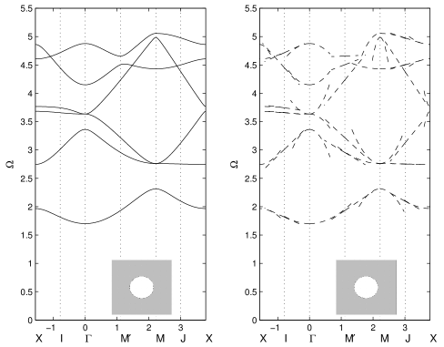
Figure 5: The solid line dispersion curves are from FE computations (circle of radius $0.4$) and the dashed are from the HFH asymptotics. These curves become virtually indistinguishable when one takes larger and larger macro cells, as this amounts to perturbing away from an increasing number of standing waves on the diagrams, which is the essence of the folding technique. In the limit of an infinite macro cell one would perturb away from a dense set of points on the diagrams, and their reconstruction would become perfect [kirill-personal].

The full dispersion curves are computed numerically using COMSOL (finite element code [comsol]) and then asymptotically with the HFH using the equations developed in section 2. Fig. 4 illustrates the typical dispersion curves versus the asymptotics for wavenumbers, on the specified path of Fig. 3, for the example of a hole with radius $0.4$. There is, as expected, a zero-frequency stop-band and the lowest branch is isolated with a full stop-band also lying above it. At some standing wave frequencies two modes share the same frequency, for instance the third and fourth modes at $\Gamma$; these modes are asymptotically quadratic in the local wavenumber. Table 2 shows the $T_{11},T_{22}$ values for point $\Gamma$ of the Brillouin zone. Note how $T_{11}=T_{22}$ for all single eigenfrequencies, but that symmetry breaks for the double roots. Moreover the signs of the $T_{11}$ and $T_{22}$ naturally inform one of the local curvature near $\Gamma$. Physically, this tells us the sign of group velocity of waves with small phase-shift across the unit cells, and thus whether or not they undergo backward propagation, which is one of the hallmarks of negative refraction.

4.1.2 Folding technique for reconstructing the dispersion curves asymptotically

An apparent deficiency of the approach we present is that it requires known standing wave frequencies, and associated eigenstates, at the band edges and that the asymptotics may be poor at frequencies far from these standing waves; until now HFH, applied to the dispersion curves, has been limited to obtaining asymptotic solutions near the standing wave frequencies [craster10a]. This uses an elementary cell containing a single hole and the irreducible Brillouin zone associated with it, however by using larger macro-cells containing four or more holes, and foldings of their resultant Brillouin zone, one can extract the asymptotics at other positions in wavenumber space thereby considerably enhancing the asymptotically coverage, see Fig. 5. As an example, we take an elementary square cell of length $2$ with circular holes of radius $0.4$, section 4.1 and Fig. 4.

To obtain asymptotic solutions at the wavenumber positions, $I(\pi/4,0)$, $J(\pi/2,\pi/4)$, $M^{\prime}(\pi/4,\pi/4)$ of Fig. 5(b), bisecting the three segments $[\Gamma X]$, $[MX]$ and $[\Gamma M]$ of the Brillouin zone we can use the equations (15, 16, 17) again, section 2.2, but now with different elementary cells.

Let the Brillouin zone for a square macro-cell composed of four holes be $\Gamma^{\prime}M^{\prime}I$. At $\Gamma^{\prime}(0,0)$ periodic (in-phase) conditions on the macro cell boundaries yield all in-phase and out-of-phase modes of the elementary cell containing a single hole. This elementary cell’s $[\Gamma M]$ segment is folded on point $M^{\prime}$. At $M^{\prime}$, where anti-periodic (out-of-phase) conditions on the macro cell are applied, the dispersion curves contain repeated roots, which are linear, and their slope is equal to the asymptote of the dispersion curves of the elementary cell setting at point $M^{\prime}$. Proceeding in a similar manner one can fold the Brillouin zone at will by considering macro-cells composed of simple unfoldings of the elementary cell. Asymptotics can be obtained for wavenumber positions of the Brillouin zone equal to all ratios of the elementary cell’s Brillouin zone wavenumber points. These ratios are equal to $1/n$ where $n$ is related to the number of elementary cells of one hole contained in the macro cell in each dimension.

We now illustrate this by obtaining asymptotics at points $M^{\prime}$, $I$ and $J$ which respectively correspond to the following macro cell settings, a square macro cell composed of four elementary cells with anti-periodic boundary conditions, a rectangular macro cell composed of two elementary cells in the $\xi_{1}$ direction with anti-periodic boundary conditions on $\xi_{1}$ but periodic on $\xi_{2}$ and finally a rectangular macro cell composed of two elementary cells in the $\xi_{2}$ direction with anti-periodic conditions in $\xi_{1}$ and $\xi_{2}$. The asymptotics at points $M^{\prime}$, $I$, $J$ as well as the usual points $\Gamma$, $M$ and $X$ are illustrated in Fig. 5.

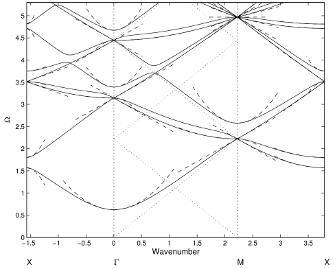
Figure 6: The dispersion curves for a doubly periodic array of constrained points: Solid lines are from exact dispersion relation (32) and the dashed lines are HFH asymptotics. Additionally, we draw two sets of dotted lines emerging from $\Gamma$ and $X$ which are folded light lines.

$T_{11}$	$T_{22}$	$\Omega_{0}$
$0.979719694474189$	$0.979724590049377$	$0.624563144241832$
$1$	$-22.34$	$\pi$
$12.439613406598808$	$12.439765169617527$	$3.388815608872719$
$-16.77$	$18.77$	$\sqrt{2}\pi$
$18.856092144598160$	$18.855405067087230$	$4.670779386112907$

Table 3: The first five frequencies for in-phase standing waves and their respective $T_{ij}$ coefficients for a doubly periodic array of square cells with zero radius holes (see Fig. 6). Equal $T_{11}$ and $T_{22}$ coefficients are for the single multiplicity eigenmodes. The second and fourth set of $T_{ij}$ are for the quadratic modes of the Dirac-like cones.

4.2 Circular inclusions of small radius

As the hole radius decreases, the dispersion curves gradually transition toward those of the infinitesimal holes shown in Fig. 6: The zero frequency stop-band is generic, and a feature forced by the Dirichlet boundary condition, however, the lowest dispersion curve is no longer isolated and triple crossings created by repeated roots occur.

For the larger hole radius, section 4.1, all the modes are locally quadratic close to the standing wave frequencies. As the wavenumber moves away from those specific Brillouin zone points the behaviour of the dispersion curves becomes locally linear. The formation of triple, and more, crossings as the radius tends to zero, are created by the linear behaviour of the dispersion curves far away from points $\Gamma$, $M$ and $X$ moving toward those points to replace the quadratic behaviour of all the multiple modes, except one, as seen in Fig. 6. Triple crossings are illustrated at the second and fourth standing wave frequencies at point $\Gamma$ and the first standing wave frequencies at point $M$, where the third frequency at point $M$ yields a hep-tuple crossing. Reassuringly, the asymptotic theory captures these multiple modes whether the crossings are double, triple, or more as is illustrated in Figs. 4, 6 where the circular holes are respectively of radius $0$ and $0.4$. For the multiple crossing points with multiplicity higher than two, both linear and quadratic dispersion curves arise. One can proceed, as in section 2.2, to obtain the different $\Omega_{1}$ coefficients and one of them is zero; proceeding to higher order and apply equations (26) to (28) gives the quadratic behaviour of the middle mode emerging from the triple crossings. Again the $T_{ii}$ contain the critical information about the local behaviour, some typical values along $\Gamma$ are given in table 3, for the quadratic curves; they are naturally identical for isolated modes but describe the inherent anisotropy for the other cases. One can then immediately see whether the material will behave with directional preferences at specific frequencies.

Dispersion diagrams of zero radius and for $0.1$ radius (not shown) geometries are almost indistinguishable by eye, but apparent triple crossings in the latter are actually a double crossing together with a single mode that has almost the same standing wave frequency. The separation of the two almost touching standing wave frequencies depends on the size of the inclusion and tends to zero as the inclusion shrinks down to a point: Fig. 7 illustrates a close-up of a triple point comparing inclusions of radius $0$ and $0.1$. This is actually important for the Dirac-like cones and associated effects.

4.3 Zero radius, Fourier series and Dirac-like cones

A doubly periodic array of constrained points (circles of zero radius) is an attractive limit and has an immediate solution in terms of Fourier series as

$$u(\xi_{1},\xi_{2})=e^{i{\bm{\kappa}}\cdot{\bm{\xi}}}\sum_{n_{1}=-\infty}^{\infty}\sum_{n_{2}=-\infty}^{\infty}\frac{e^{-i\pi{\bf N}\cdot{\bm{\xi}}}}{(\kappa_{1}-\pi n_{1})^{2}+(\kappa_{2}-\pi n_{2})^{2}-\Omega^{2}}$$ (31)

with ${\bm{\kappa}}=(\kappa_{1},\kappa_{2})$ and ${\bf N}=(n_{1},n_{2})$ and $\Omega$ and $\bm{\kappa}$ are related via the dispersion relation

$$D({\bm{\kappa}},\Omega)=\sum_{n_{1}=-\infty}^{\infty}\sum_{n_{2}=-\infty}^{\infty}\frac{1}{(\kappa_{1}-\pi n_{1})^{2}+(\kappa_{2}-\pi n_{2})^{2}-\Omega^{2}}=0.$$ (32)

This is valid provided the double sum does not have a singularity, which would occur whenever

$$\Omega=\sqrt{(\kappa_{1}-\pi n_{1})^{2}+(\kappa_{2}-\pi n_{2})^{2}}.$$ (33)

These relations from the singularities also play a role in the dispersion picture; they correspond to the Bloch states of a perfect medium without any constraints (a homogeneous isotropic medium). However, in some circumstances they also, by serendipity, exactly satisfy the constraint $u=0$ at the centre of each cell and therefore, in those cases, are simultaneously dispersion curves; this is the origin of the degeneracy seen in the multiple crossings (occurring at Dirac-like points) of the dispersion curves of Fig. 6. It is also clear from the dispersion relation that $\Omega=0$ is not a solution at $\bm{\kappa}={\bf 0}$ and hence that there is a zero-frequency stopband and conventional long-wave homogenization is doomed to failure cf. section 2.1.

A set of dispersion curves are shown in Fig. 6: The Bloch states for the perfect medium free of defects lead to light lines folded at the edges of the Brillouin zone and those emerging from $\Gamma$ are pertinent to the current discussion. These light lines intersect at the multiple crossings, which are called generalized Dirac-like points: Generalized Dirac-like points occur for a given set of frequencies at all three edges of the Brillouin zone, namely for points $\Gamma$, $M$ and $X$. It is useful to find criteria for their multiplicity: At $\Gamma$ the generalized Dirac-like points occur for $\Omega^{2}=\pi^{2}m$ such that $m=n_{1}^{2}+n_{2}^{2}$ with $m$ integer; the multiplicity depends on the ways in which $n_{1}$ and $n_{2}$ can form $m$. From elementary number theory $m$ can be equal to the sum of two squares in more than one way, i.e., $m=50=5^{2}+5^{2}=7^{2}+1^{2}$ or the sum of two squares can also be a perfect square, i.e., $m=25=5^{2}=4^{2}+3^{2}$. Equation $u_{,x_{i}x_{i}}+\pi^{2}(n_{1}^{2}+n_{2}^{2})u=0$ together with the appropriate boundary conditions describes the generalized Dirac-like points and an independent set of solutions is formed from different possibilities of $\sin(\pi(n_{i}x+n_{j}y))$, $\sin(\pi(n_{i}x-n_{j}y))$, $\cos(\pi(n_{i}x+n_{j}y))$-$\cos(\pi(n_{p}x-n_{k}y))$ where $i,j,p,k\in\{1,2\}$, $i\neq j$ and $p\neq k$. The multiplicity can be equal to $3$, $7$, $11$ or more depending on $m$. For example $\Omega^{2}=\pi^{2}$ with $n_{i}=1$, $n_{j}=0$ has multiplicity $3$ where $\Omega^{2}=5\pi^{2}$ has multiplicity $7$ and $\Omega^{2}=50\pi^{2}$ has multiplicity $11$. This is true for solutions at $\Gamma$ and $M$ but at $X$ one can obtain a singularity that accepts only one eigensolution. Due to the non-symmetry of the general sum at $X$ that renders the denominator of the Fourier series singular, $m=(1/2-n_{1})^{2}+n_{2}^{2}$, it is possible to obtain solutions of multiplicity one as in the case of $\Omega_{0}=\pi/2$ where the only eigensolution respecting the boundary conditions is $\sin(\pi x/2)$.

Given the exact solution one can, in these special cases, generate the asymptotics by hand. For the asymptotics we construct the coefficients using $U_{0}$ from (31) and deduce ${\bf U}_{1}=(U_{11},U_{12})$ as

$$U_{1k}=2ie^{i{\bm{\kappa}}\cdot{\bm{\xi}}}\sum_{n_{1}=-\infty}^{\infty}\sum_{n_{2}=-\infty}^{\infty}\frac{(\kappa_{k}-\pi n_{k})e^{-i\pi{\bf N}\cdot{\bm{\xi}}}}{[(\kappa_{1}-\pi n_{1})^{2}+(\kappa_{2}-\pi n_{2})^{2}-\Omega^{2}]^{2}}$$ (34)

and thus one can extract the $T_{ij}$ in (15) by doing the integrals by hand, the off-diagonal terms are zero, and $T_{11}$ and $T_{22}$ are

$$T_{11}=1-4\frac{\sum_{n_{1}=-\infty}^{\infty}\sum_{n_{2}=-\infty}^{\infty}\frac{(\kappa_{1}-\pi n_{1})^{2}}{[(\kappa_{1}-\pi n_{1})^{2}+(\kappa_{2}-\pi n_{2})^{2}-\Omega_{0}^{2}]^{3}}}{\sum_{n_{1}=-\infty}^{\infty}\sum_{n_{2}=-\infty}^{\infty}\frac{1}{[(\kappa_{1}-\pi n_{1})^{2}+(\kappa_{2}-\pi n_{2})^{2}-\Omega_{0}^{2}]^{2}}},\quad\\$$ (35)

and an identical equation for $T_{22}$ but with $1$ and $2$ interchanged, where $(\kappa_{1},\kappa_{2})$ are $(0,0)$, $(\pi/2,0)$ and $(\pi/2,\pi/2)$ at the edges of the Brillouin zone at the respective points of $\Gamma$, $X$ and $M$. These asymptotics only apply at the isolated, non-repeating roots, and are shown in Fig. 6.

The linear cases at the triple crossings are easily extracted from section 2.2. For instance, for the repeated case at $\Omega_{0}=\pi$ there are three linearly independent solutions with

$$u_{0}=f^{(1)}({\bf X})\sin\pi\xi_{1}+f^{(2)}({\bf X})\sin\pi\xi_{2}+f^{(3)}({\bf X})[\cos\pi\xi_{1}-\cos\pi\xi_{2}]$$ (36)

Following through the methodology one arrives at $2\Omega_{1}^{4}=(2\pi)^{2}(\kappa_{1}^{2}+\kappa_{2}^{2})$ which gives the two linear asymptotics, and similarly at the other points. Table 1 summarizes the coefficients for the first two Dirac-like cones at point $\Gamma$. The asymptotics are shown in Fig. 7 showing that the linear behaviour is perfectly captured.

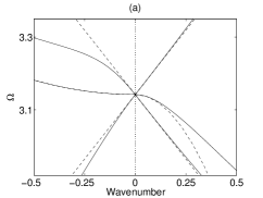
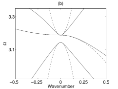
Figure 7: Panel (a) shows a close up of the Dirac-like point and its asymptotics from figure 6. The values for the asymptotic coefficients of equation (25) are $\alpha_{11}=\alpha_{22}=2\pi^{2}$ and for equation (18) they are $T_{11}=1$ and $T_{22}=-22.34$. Panel (b) shows the same region for a slightly larger hole radius of $0.1$ where one can see the merging of the double mode with the mode near $\pi$ to form a triplet as the radius decreases to zero. HFH captures both cases as is seen from the asymptotic curves. As the radius decreases the top and bottom quadratics become steeper and ultimately reach a linear behaviour.

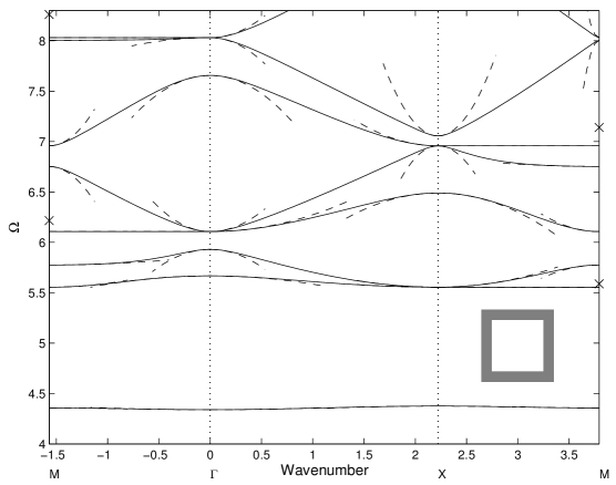
Figure 8: The dispersion curves for square inclusions, of side $\sqrt{2}$, from numerical simulation (solid) and from HFH theory (dashed). The HFH and numerics for the lowest two curves are virtually indistinguishable. The crosses on the frequency axis are frequencies predicted by solving Helmholtz’s equation in a waveguide consisting of a rectangle with Neumann data on one side and Dirichlet data on the other sides, see also Figure. 10. Their values in increasing order are $5.59$, $6.22$, $7.14$ and $8.26$.

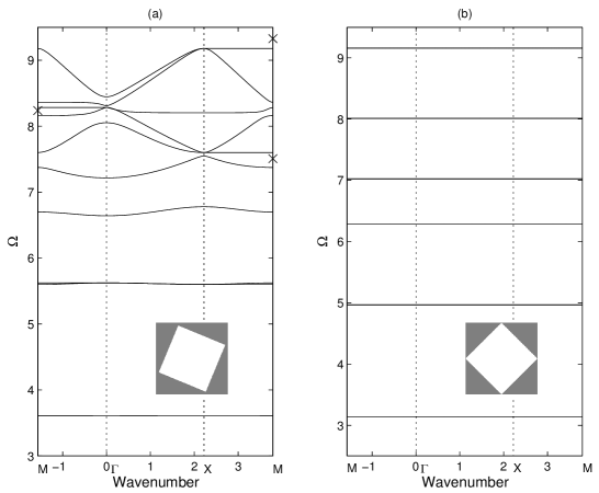
Figure 9: The dispersion curves for a square of side $\sqrt{2}$ from numerical simulation for (a) a square rotated by $\pi/8$ and (b) by $\pi/4$. The crosses on the frequency axis in (a) are frequencies predicted by solving Helmholtz’s equation in a waveguide. Their values are $7.51$, $8.24$ and $9.33$.

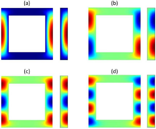
Figure 10: The eigenstates of the first four flat bands at the respective frequencies of $5.56$, $6.11$, $6.96$ and $8.03$. The left of every panel shows FEM computations of the eigenstate, as noted in the text a waveguide model can be developed to approximate the field and eigenvalue and these waveguide counterparts are shown alongside.

4.4 Square inclusions

Our methodology is not limited to circular inclusions and is easily applied to any shape, we briefly consider square inclusions taking a square of side $\sqrt{2}$ and see in Fig. 8 that the dispersion curves are not unlike those of the large cylinder in Fig. 4: an isolated lowest mode separating a zero frequency stop-band from a wide stop-band, yet another stop band arises near $\Omega=6$. The asymptotics from HFH again reproduce the behaviour near the edges of the Brillouin zone and can be used to construct effective HFH equations. The HFH results in Fig. 4 are almost completely indistinguishable all along the lowest two branches and are highly accurate near the edges of the Brillouin zone for the other branches. Interestingly, the orientation of the square matters strongly and rotating it progressively flattens the lowest (lower frequency) dispersion curves until ultimately, for a rotation of $\pi/4$, they become completely flat leading to resonant states: The rotation gradually isolates each piece of material from its neighbours leaving resonant blocks that vibrate with the eigenfrequency of Dirichlet squares of side $\sqrt{2}$ $\Omega^{2}=(m\pi/\sqrt{2})^{2}+(n\pi/\sqrt{2})^{2}$ with $m,n$ non-zero integers.

4.4.1 Standing wave modes

It is noticable in Figs. 8 and 9a that completely flat modes exist which represent standing waves for a whole range of Bloch wavenumbers. The eigenfunctions, for the non-tilted case, for the first four standing wave frequencies, are shown in Fig. 10; it is clear that the field is concentrated along parallel and opposite sides and this suggests a simple equivalent waveguide model can be constructed. Taking a rectangle with a Neumann condition on one side and Dirichlet conditions on the other three sides where the Neumann condition on one side is necessary to cover the appropriate symmetry. The length and width of the rectangle depends on the tilt of the square hole. For the non-tilted case the length is taken to be the length of a cell and the width as the half width of the cell minus the inner square. The resulting frequency estimate $\Omega_{E}$ reads,

$$\Omega_{E}=\pi\left(\left(\frac{2n-1}{l-w}\right)^{2}+\left(\frac{m}{l}\right)^{2}\right)^{\frac{1}{2}}\quad\text{for}\quad n,m\in\mathbb{N}^{*}$$ (37)

where $l$ and $w/2$ are respectively the effective length and width of the waveguide. For the non-tilted square hole $l_{0}=2$ and $w_{0}=2-\sqrt{2}$ where for a tilt of $\pi/8$ they reduce to the values of $l_{\pi/8}=1.6051$ and $w_{\pi/8}=0.4335$. Equation (37) then leads to the ’x’ crosses placed on Figs. 8 and 9a which are good predictions of the standing wave frequencies, and the approximate eigensolutions are shown in Fig. 10. The precision of the estimates degenerates as the frequency increases as the field near the ends of the imaginary rectangle gradually leaks into the undisturbed ligaments.

5 Lensing, guiding and cloaking effects

We now connect the HFH theory with the exciting phenomena that are topical in photonics.

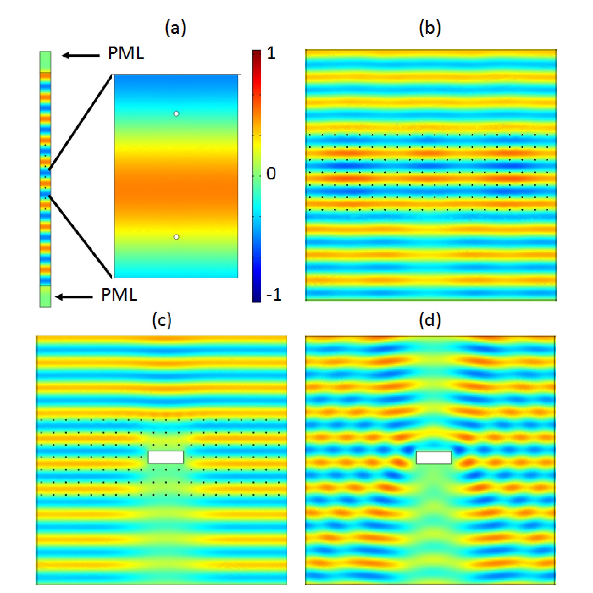
Figure 11: Dirac-like cone versus cloaking: (a) Perfect transmission through a column of seven constrained evenly spaced inclusions of radius $0.01$ (array pitch $2$) with periodic conditions on either sides and Perfectly Matched Layers (PML) on top and bottom, and a plane wave incident from above at frequency $\Omega_{0}=2.215$; (b) Nearly perfect transmission for a plane wave at frequency $\Omega_{0}$ incident from above on a finite array of $140$ constrained inclusions with PML on either sides of the computational domain; (c) Same as in panel (b) when a clamped rectangular obstacle is placed inside the array; (d) Plane wave incident from above on the clamped obstacle at frequency $\Omega_{0}$ for comparison; The slightly reduced amplitude in forward scattering in (c), but the lack of backward scattering, is a hallmark of cloaking.

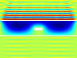
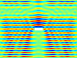
Figure 12: Panel (a) shows nearly perfect transmission for a plane wave at frequency $\Omega_{0}$ incident from above on an effective medium with properties computed by HFH for a frequency near $\Omega_{0}=2.215$ with PML on either sides of the computational domain; A Plane wave incident from above on the clamped obstacle at frequency $\Omega_{0}$ for comparison.

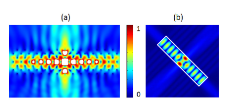
Figure 13: Lensing effects in a PC (tilted array) of small Dirichlet holes: (a) Lensing for a line source inside the PC at frequency $\Omega=2.7$; (b) Using equation (29) the PC is replaced by an effective medium in order to yield the same effect as in (a).

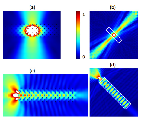
Figure 14: Guiding and lensing effects in a PC (tilted array) of small Dirichlet holes: (a) Omni-directive antenna for a line source inside the PC at frequency $\Omega=\pi/2$; (b) The PC of (a) is replaced by an effective medium obtained by HFH with equation (29) in order to obtain the same physical effect; (c) Endoscope for a line source at $\Omega=2.7$; (d) The PC of (c) is replaced by an effective medium using equation (30) to obtain the same physical effect.

5.1 Cloaking effects near Dirac-like cones

As noted in recent articles [chan12a] a curious phenomenon occurs in photonics near Dirac-like points which are the triple crossings shown in, for instance, Fig. 7. Let us consider the lowest frequency triple point, near wavenumber $M$, shown in Fig. 6; for the full finite element numerical simulations we actually consider very small cylinders of radius $0.01$ in a square array. The triple crossings occur because the dispersion relation of a perfect medium (no cylinders) consists of light lines folded in space (one folded light line is shown in Fig. 6). The folded light lines happen to satisfy the boundary condition for the infinitesimal point holes, and are perturbed slightly for finite cylinders (as in Fig. 7); the middle curve passing between the Dirac-like cone is created by the inclusion and so these effects co-exist. Importantly, this means that there is near perfect transmission through an array of cylinders close to these triple crossing frequencies as shown in Fig. 11(a,b) as the incoming plane wave, at $\Omega=2.215$, does not see the inclusions. Inserting a large Dirichlet hole within the array leads to virtually no reflection, the plane wave is hardly reflected, and its transmission is nearly perfect Fig. 11(c) except for a slight shadow zone in clear contrast to the uncloaked Dirichlet hole Fig. 11(d); If we remove the array of small holes, the defect is strongly scattered by the wave.

Replacing the array of holes with HFH is shown in Fig. 12 the quasiperiodic medium is replaced by a homogeneous medium with the effective properties given by HFH. The excitation is at a frequency $\Omega=2.12$, close to the standing wave frequency $\Omega_{0}$. Inserting the values for $l=1$, $\Omega_{0}$, $\Omega$ and $\beta=2/\pi^{2}$ into equation (30) we obtain the effective continuum equation,

$${\hat{f}}_{0,x_{i}x_{i}}({\bf x})+0.0393{\hat{f}}_{0}({\bf x})=0.$$ (38)

Simulations show qualitatively the same effects, one has transmission through the slab with plane waves incoming.

5.2 Lensing and wave guiding effects

Returning to the introduction we show in Fig. 2(a,c) a PC composed of an array of $196$ holes with radius $0.4$; the corresponding dispersion curves are shown in Fig. 4.

We now interpret these strongly anisotropic beams and how the HFH represents this. In Fig 2 (a,b) we choose frequency $\Omega=1.98$, which from Fig. 4 is near the standing wave frequency $\Omega_{0}=1.966$ at point $X(\pi/2,0)$. The reciprocal space is only shown for a portion of the irreducible Brillouin zone and one can use reflections of the triangle chosen to fill the entire square in the Brillouin zone; due to these internal symmetries the effect is not only due to the first mode of Fig. 4 at point $X(0,\pi/2)$ of the reciprocal space, but also to the first mode, at point $G(\pi/2,0)$ (not shown). The effect is reproduced in Fig. 2 (b) by combining two effective medium equations, one for point $X$ and one for point $G$, each one is responsible for a single diagonal, and the HFH equations are

$$\quad-1.4778{\hat{f}}_{0,x_{1}x_{1}}({\bf x})+0.8837{\hat{f}}_{0,x_{2}x_{2}}({\bf x})+(\Omega^{2}-\Omega_{0}^{2}){\hat{f}}_{0}({\bf x})=0,$$ (39)

$$\quad 0.8837{\hat{f}}_{0,x_{1}x_{1}}({\bf x})-1.4778{\hat{f}}_{0,x_{2}x_{2}}({\bf x})+(\Omega^{2}-\Omega_{0}^{2}){\hat{f}}_{0}({\bf x})=0,$$ (40)

with $(\Omega^{2}-\Omega_{0}^{2})=0.0552$. Note that these effective equations have opposite signs in the coefficient, and so the governing equations are hyperbolic and not elliptic, the result is that these direct energy along rays or characteristics and the angle is given by the relative magnitude of the $T_{11}$ and $T_{22}$; in this case roughly equal with the energy directly along the diagonals.

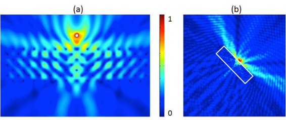
Figure 15: Lensing effects in a PC (tilted array) of small Dirichlet holes acting as a flat lens near a frequency of $\pi/2$: (a) A line source near the top of the PC yields an image on the other side. The PC is composed of $96$ very small holes arranged in a tilted square array with an angle of $\pi/4$. (b) shows clearly the same effect happening when the PC is replaced by a anisotropic effective medium obtained through HFH.

To illustrate this further in panel (c) of Fig. 2 we show a St George’s cross effect obtained near the standing wave frequency $\Omega_{0}=2.744$. By homogenizing the PC and exciting it at a frequency of $\Omega=2.75$ we obtain two effective medium equations, one for $X$ and one for $G$ that are,

$$\quad 3.1094{\hat{f}}_{0,x_{1}x_{1}}({\bf x})+0.085{\hat{f}}_{0,x_{2}x_{2}}({\bf x})+(\Omega^{2}-\Omega_{0}^{2}){\hat{f}}_{0}({\bf x})=0,$$ (41)

$$\quad 0.085{\hat{f}}_{0,x_{1}x_{1}}({\bf x})+3.1094{\hat{f}}_{0,x_{2}x_{2}}({\bf x})+(\Omega^{2}-\Omega_{0}^{2}){\hat{f}}_{0}({\bf x})=0.$$ (42)

Each equation is responsible for a single line of the cross, the orientation of this cross is explained by the almost zero coefficient, in each effective equation, that does not permit propagation in the vertical and horizontal direction for the respective equations (41) and (42). The coefficient in front of ${\hat{f}}_{0}({\bf x})$ is equal to $0.033$. It is clear therefore that the strong anisotropy that is witnessed in full FE numerical simulations has its origins in the size and sign of the $T_{ij}$ coefficients from HFH and the effective equations can be used to gain quantitative understanding and predictions.

Another striking application involving wave propagation and an array of small holes of radius $0.01$ is shown in Figs. 13, 14 , 15 wherein we have tilted the array through an angle $\pi/4$. The dispersion curves in Fig. 6 are for holes of radius exactly zero, but provide very good comparison for this small holes case.

We obtain a highly-directed emission at frequency $\Omega=1.6$ near the standing wave frequency $\Omega_{0}=\pi/2$, shown in Fig. 14(a) with its effective medium counterpart in 14(b); in the dispersion curves this is the lowest standing wave frequency at $X$. There are two effective medium equations at this frequency which yield,

$$\quad-11.42{\hat{f}}_{0,x_{1}x_{1}}({\bf x})+{\hat{f}}_{0,x_{2}x_{2}}({\bf x})+(\Omega^{2}-\Omega_{0}^{2}){\hat{f}}_{0}({\bf x})=0,$$ (43)

$$\quad{\hat{f}}_{0,x_{1}x_{1}}({\bf x})-11.42{\hat{f}}_{0,x_{2}x_{2}}({\bf x})+(\Omega^{2}-\Omega_{0}^{2}){\hat{f}}_{0}({\bf x})=0,$$ (44)

where the difference of the frequency squares is equal to $0.0926$. For forcing within the slab one again has a strongly anisotropic response, the waves within the medium forming a cross-shape which, when it strikes the edge of slab all gets radiated out into the surrounding medium. Placing a source outside the slab, again at a frequency near $\Omega_{0}=\pi/2$, Fig. 15(a) shows a PC that behaves like a flat lens. In panel (b) of that Fig. the effective medium yields the same effect and is also governed by two equations of the form of (29) with $T_{ij}$ coefficients equal to the ones of equation (44). The frequency at which the lensing effect is obtained is $\Omega=1.56$ and so the coefficients in front of ${\hat{f}}_{0}({\bf x})$ are equal to $-0.0338$ in this case.

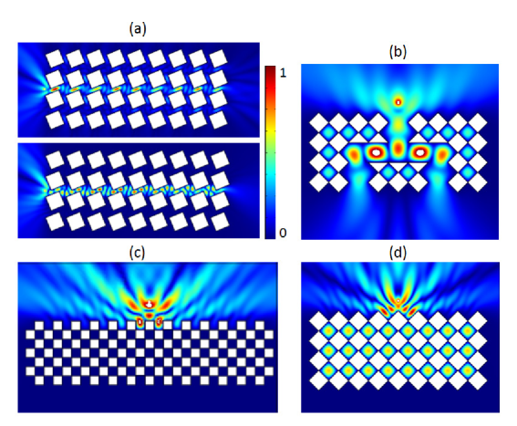
Figure 16: Lensing and guiding effect through a PC composed of square Dirichlet holes which we vary their tilt angle: (a) Lensing effects in a PC composed of Dirichlet square holes tilted by $\pi/8$ near the respective frequencies of $7.7$ and $8.25$ for the top and bottom figures (Fig 9a). (b) The dispersion curves in Fig. 9b show the band structure is composed of many band gaps separated by standing wave modes, so that the structure acts as a perfect reflector for any frequency in order to guide light. (c) shows a perfect reflector for a source exciting the medium at frequency $4.95$, located in the second band gap of Fig. 8. (d) shows the same effect as in (c) for a frequency of $5.0$ although in the present the filled parts of material are excited but no energy escapes the PC and acts as an energy trap.

Figs. 13(a) and 14(c) show lensing effects where the PC is excited at $\Omega=2.7$, this frequency is chosen as follows: When the array is rotated the relevant light line in the surrounding material, and its folding, emerge from the point $M$ and are shown in Fig. 6 we see that the energy from the source couples (as the light line crosses the full dispersion curves at $\Omega=2.7$) into one of the linear Dirac-like cone modes that passes through $\Omega_{0}=\pi$; this is the standing wave frequency of the Dirac-like cone at $\Gamma$. We therefore model the effective medium with HFH using the analysis near $\Omega=\pi$, and it yields very similar results in Figs. 13(b) and 14(d), by homogenizing the PC with an effective material governed by equation,

$${\hat{f}}_{0,x_{i}x_{i}}({\bf x})+0.3371{\hat{f}}_{0}({\bf x})=0,$$ (45)

obtained by simply replacing the source and standing wave frequencies together with $\beta=1/(2\pi^{2})$ in equation (30).

Finally, Fig. 16(a) shows a unidirective PC for the first two flat modes of the band diagram in Fig. 9(a). The standing wave frequencies of the two flat modes in question are $\Omega_{0}=7.6$ and $\Omega_{0}=8.28$. The sources are excited near these frequencies at $\Omega=7.7$ and $\Omega=8.25$. HFH yields effective medium equations for each of the modes that are respectively,

$$\quad 9.3649{\hat{f}}_{0,x_{1}x_{1}}({\bf x})+(\Omega^{2}-\Omega_{0}^{2}){\hat{f}}_{0}({\bf x})=0,$$ (46)

and

$$\quad-45.8434{\hat{f}}_{0,x_{1}x_{1}}({\bf x})+(\Omega^{2}-\Omega_{0}^{2}){\hat{f}}_{0}({\bf x})=0,$$ (47)

Equations (46) and (47) clearly show the unidirectivity of the two effective media. Similar equations with interchanged coeffcients stand, for the symmetric location of the Brillouin zone $G(0,\pi/2)$. Panels (b), (c) and (d) contain PCs with rotated square holes by an angle of $\pi/4$ with an unsual band diagram seen in Fig. 9(b). Panel (b) shows the guiding of a wave by means of perfect reflection for a line source excitated just outside the standing wave frequency of $\Omega=4.95$ while in panel (c) the same PC but this time rotated by an angle of $\pi/2$ acts as a perfect reflector. Panel (d) finally excites the medium right on the standing wave frequency of $\Omega=5$ and standing waves appear between the holes. Small gaps between the hole’s edges make it possible for energy to pass from one cell to the other.

6 Concluding remarks

In this paper, we have presented a range of applications of the high frequency homogenization theory, in the context of zero-frequency stop band structures, which were previously thought to be non-homogenizable: HFH has succeeded in capturing the finer details of both dilute and densely packed photonic and phononic crystals. Striking physical effects such as cloaking via Dirac-like cones and directive antennas and endoscope effects have been provided, and fully explained, via HFH; importantly this is all shown to be related to the potentially anisotropic $T_{ij}$ coefficients that encode the local behaviour or their equivalent terms for multiple crossings. The range of unsolved homogenization problems in the wave community is vast, and this new method now opens the door to efficient simulation of multiscale structures.

The current theory is limited to periodic, or nearly periodic media, however one can envisage extensions in a variety of different directions: In this paper we deal with photonic and phononic periodic structures, but it should be possible to adapt our results to quasi-crystals using a generalized form of the Floquet-Bloch theorem in upper dimensional spaces. Stochastic cases where the hole positions involve some random perturbation, say, might prove more arduous from a mathematical standpoint, although a physicist might argue the period would be replaced by the mean distance between the inclusions. The key point in order to relax the constraint of classical homogenization is the assumption that the Floquet-Bloch theorem is applicable at least to leading order. Whenever this can be done, or an extension of the Floquet-Bloch theorem can be used, HFH is applicable. Also of interest are diffusion problems in composites, classic homogenization is here again constrained by low frequencies (e.g. of a periodic heat source), whereas much of the exciting physics lies beyond the quasi-static regime again we hope that the insight provided by HFH will lead to progress in these directions.

References

References

- [1] \harvarditemAllaire \harvardand Piatnitski2005allaire05a Allaire G \harvardand Piatnitski A 2005 Commun. Math. Phys. 258, 1–22.
- [2] \harvarditemAntonakakis \harvardand Craster2012antonakakis12a Antonakakis T \harvardand Craster R V 2012 Proc. R. Soc. Lond. A 468, 1408–1427. doi: 10.1098/rspa.2011.0652.
- [3] \harvarditemAntonakakis et al.2013aantonakakis13a Antonakakis T, Craster R V \harvardand Guenneau S 2013a Proc. R. Soc. Lond. A 469, 20120533.
- [4] \harvarditemAntonakakis et al.2013bantonakakis13b Antonakakis T, Craster R V \harvardand Guenneau S 2013b Moulding and shielding flexural waves in elastic plates. under review.
- [5] \harvarditemBensoussan et al.1978bensoussan78a Bensoussan A, Lions J \harvardand Papanicolaou G 1978 Asymptotic analysis for periodic structures North-Holland, Amsterdam.
- [6] \harvarditemBirman \harvardand Suslina2006birman06a Birman M S \harvardand Suslina T A 2006 Journal of Mathematical Sciences 136, 3682–3690.
- [7] \harvarditemBouchitté \harvardand Felbacq2004bouchitte04a Bouchitté G \harvardand Felbacq D 2004 Comptes Rendus Mathématique 339, 377–382.
- [8] \harvarditemBrule et al.2013brule13a Brule S, Javelaud E, Enoch S \harvardand Guenneau S 2013 Seismic metamaterial: How to shake friends and influence waves? under review.
- [9] \harvarditemChan et al.2012chan12a Chan C T, Huang X, Liu F \harvardand Hang Z H 2012 Progress In Electromagnetic Research 44, 163–190.
- [10] \harvarditemCherednichenko2012kirill-personal Cherednichenko K 2012. Personal communication.
- [11] \harvarditemCherednichenko et al.2006cherednichenko06a Cherednichenko K D, Smyshlyaev V P \harvardand Zhikov V V 2006 Proc. Roy. Soc. Edinburgh 136 A, 87–114.
- [12] \harvarditemCOMSOL2012comsol COMSOL 2012 www.comsol.com.
- [13] \harvarditemConca et al.1995conca95a Conca C, Planchard J \harvardand Vanninathan M 1995 Fluids and Periodic structures Res. Appl. Math., Masson, Paris.
- [14] \harvarditemCraster et al.2012craster12b Craster R V, Antonakakis T, Makwana M \harvardand Guenneau S 2012 Phys. Rev. B 86, 115130.
- [15] \harvarditemCraster \harvardand Guenneau2013craster12a Craster R V \harvardand Guenneau S, eds 2013 Acoustic Metamaterials Springer-Verlag.
- [16] \harvarditemCraster et al.2011craster11a Craster R V, Kaplunov J, Nolde E \harvardand Guenneau S 2011 J. Opt. Soc. Amer. A 28, 1032–1041.
- [17] \harvarditemCraster et al.2010craster10a Craster R V, Kaplunov J \harvardand Pichugin A V 2010 Proc R Soc Lond A 466, 2341–2362.
- [18] \harvarditemFarhat et al.2010farhat10b Farhat M, Guenneau S \harvardand Enoch S 2010 European Physics Letters 91, 54003.
- [19] \harvarditemGuenneau et al.2007guenneau07b Guenneau S, Ramakrishna S A, Enoch S, Chakrabarti S, Tayeb G \harvardand Gralak B 2007 Photonics and Nanostructures – Fundamentals and Applications 5, 63–72.
- [20] \harvarditemGuenneau \harvardand Zolla2000zolla00a Guenneau S \harvardand Zolla F 2000 Progress In Electromagnetic Research 27, 91–127.
- [21] \harvarditemHoefer \harvardand Weinstein2011hoefer11a Hoefer M A \harvardand Weinstein M I 2011 SIAM J. Math. Anal. 43, 971–996.
- [22] \harvarditemJikov et al.1994jikov94a Jikov V, Kozlov S \harvardand Oleinik O 1994 Homogenization of differential operators and integral functionals Springer-Verlag.
- [23] \harvarditemJoannopoulos et al.2008joannopoulos08a Joannopoulos J D, Johnson S G, Winn J N \harvardand Meade R D 2008 Photonic Crystals, Molding the Flow of Light second edn Princeton University Press, Princeton.
- [24] \harvarditemJohn1987john87a John S 1987 Phys. Rev. Lett. 58, 2486–2489.
- [25] \harvarditemLiu et al.2013yan2013a Liu Y, Guenneau S \harvardand Gralak B 2013 arXiv:1210.6171 .
- [26] \harvarditemLuo et al.2002luo02a Luo C, Johnson S G \harvardand Joannopoulos J D 2002 Physical Review B 65, 201104.
- [27] \harvarditemMarkos \harvardand Soukoulis2008markos08a Markos P \harvardand Soukoulis C M 2008 Wave propagation from electrons to photonic crystals and left-handed materials Princeton University Press.
- [28] \harvarditemMcPhedran \harvardand Nicorovici1997mcphedran97a McPhedran R C \harvardand Nicorovici N A 1997 J. Elect. Waves and Appl. 11, 981–1012.
- [29] \harvarditemMilton2002milton02a Milton G W 2002 The Theory of Composites Cambridge University Press Cambridge.
- [30] \harvarditemMilton \harvardand Nicorovici2006milton06a Milton G W \harvardand Nicorovici N A 2006 Proc. Roy. Lond. A 462, 3027.
- [31] \harvarditemMovchan et al.2002movchan02a Movchan A B, Movchan N V \harvardand Poulton C G 2002 Asymptotic Models of Fields in Dilute and Densely Packed Composites ICP Press, London.
- [32] \harvarditemNemat-Nasser et al.2011nematnasser11a Nemat-Nasser S, Willis J R, Srivastava A \harvardand Amirkhizi A V 2011 Phys. Rev. B 83, 104103.
- [33] \harvarditemNicorovici et al.1995nicorovici95a Nicorovici N A, McPhedran R C \harvardand Botten L C 1995 Phys. Rev. Lett. 75, 1507–1510.
- [34] \harvarditemNotomi2000notomi00 Notomi N 2000 Phys. Rev. B 62, 10696–10705.
- [35] \harvarditemO’Brien \harvardand Pendry2002obrien02a O’Brien S \harvardand Pendry J B 2002 J. Phys. Cond. Mat. 14, 4035–4044.
- [36] \harvarditemPaul et al.2011paul11 Paul T, Menzel C, Smigaj W, Rockstuhl C, Lalanne P \harvardand Lederer F 2011 Phys. Rev. B 84, 115142–1–115142–10.
- [37] \harvarditemPendry2004pendry04b Pendry J B 2004 Science 306, 1353–1355.
- [38] \harvarditemPendry et al.1996pendry96a Pendry J B, Holden A J, Robbins D J \harvardand Stewart W J 1996 Phys. Rev. Lett. 76, 4773–4776. doi:10.1103/PhysRevLett.76.4773.
- [39] \harvarditemPendry et al.1999pendry99a Pendry J B, Holden A J, Stewart W J \harvardand Youngs I 1999 IEEE Trans. Micr. Theo. Tech. 47, 2075.
- [40] \harvarditemPoulton et al.2001poulton01a Poulton C G, Botten L C, McPhedran R C, Nicorovici N A \harvardand Movchan A B 2001 SIAM J. Appl. Math. 61, 1706–1730.
- [41] \harvarditemRamakrishna2005sar_rpp05 Ramakrishna S A 2005 Rep. Prog. Phys. 68, 449–521.
- [42] \harvarditemRayleigh1892rayleigh92a Rayleigh J W S 1892 Phil. Mag. 34, 481–502.
- [43] \harvarditemSilveirinha \harvardand Fernandes2005silveirinha05a Silveirinha M G \harvardand Fernandes C A 2005 IEEE Trans. Microwave Theory and Techniques 53, 1418–1430.
- [44] \harvarditemSmith et al.2004smith04a Smith D R, Pendry J B \harvardand Wiltshire M C K 2004 Science 305, 788–792.
- [45] \harvarditemWellander \harvardand Kristensson2003wellander03 Wellander N \harvardand Kristensson G 2003 SIAM J. Appl. Math. 64, 170–195.
- [46] \harvarditemYablonovitch1987yablonovitch87a Yablonovitch E 1987 Phys. Rev. Lett. 58, 2059.
- [47] \harvarditemZengerle1987zengerle87a Zengerle R 1987 J. Mod. Opt. 34, 1589–1617.
- [48] \harvarditemZhikov2000zhikov00a Zhikov V V 2000 Sb. Math. 191, 973–1014.
- [49] \harvarditemZolla et al.2005zolla05a Zolla F, Renversez G, Nicolet A, Kuhlmey B, Guenneau S \harvardand Felbacq D 2005 Foundations of photonic crystal fibres Imperial College Press, London.
- [50]