n-particle quantum statistics on graphs

Abstract

We develop a full characterization of abelian quantum statistics on graphs. We explain how the number of anyon phases is related to connectivity. For $2$-connected graphs the independence of quantum statistics with respect to the number of particles is proven. For non-planar $3$-connected graphs we identify bosons and fermions as the only possible statistics, whereas for planar $3$-connected graphs we show that one anyon phase exists. Our approach also yields an alternative proof of the structure theorem for the first homology group of $n$-particle graph configuration spaces. Finally, we determine the topological gauge potentials for $2$-connected graphs.

1 Introduction

In classical mechanics, particles are considered distinguishable. Therefore, the $n$-particle configuration space is the Cartesian product, $M^{\times n}$, where $M$ is the one-particle configuration space. By contrast, in quantum mechanics elementary particles may be considered indistinguishable. This conceptual difference in the description of many-body systems prompted Leinaas and Myrheim LM77 (see also S70 ; W90 ) to study classical configuration spaces of indistinguishable particles, $C_{n}(M)$, and led to the discovery of anyon statistics.

Indistinguishability of classical particles places constraints on the usual configuration space, $M^{\times n}$. Configurations that differ by particle exchange must be identified. One also assumes that two classical particles cannot occupy the same configuration. Consequently, the classical configuration space of $n$ indistinguishable particles is the orbit space $C_{n}(M)=(M^{\times n}-\Delta)/S_{n}$, where $\Delta$ corresponds to the configurations for which at least two particle are at the same point in $M$, and $S_{n}$ is the permutation group.

Significantly, the space $C_{n}(M)$ may have non-trivial topology. One can, for example, easily calculate that for $n$ particles in $M=\mathbb{R}^{N}$ the first homology group $H_{1}(C_{n}(\mathbb{R}^{N}))$ is $\mathbb{Z}$ if $N=2$ and $\mathbb{Z}_{2}$ when $N\geq 3$ D85 ; S12 . This fact, combined with the standard quantization procedure on topologically non-trivial configuration spaces, explains, at a kinematic level, the existence of anyons in two dimensions and only bosons or fermions in higher dimensions. It also raises the question of what quantum statistics are possible on spaces with richer topology.

In order to explore how the quantum statistics picture depends on topology, the case of two indistinguishable particles on a graph was studied in JHJKJR (see also BE92 ). A graph $\Gamma$ is a network consisting of vertices (or nodes) connected by edges. Quantum mechanically, one can either consider the one-dimensional Schrödinger operator acting on the edges, with matching conditions for the wave functions at the vertices, or a discrete Schrödinger operator acting on connected vertices (i.e. a tight-binding model on the graph). Such systems are of considerable independent interest and their single-particle quantum mechanics has been studied extensively in recent years Berkolaiko13 . The extension of this theory to many-particle quantum graphs was another motivation for JHJKJR (see also Bolte13 ). The discrete case turns out to be significantly easier to analyse, and in this situation it was found that a rich array of anyon statistics are kinematically possible. Specifically, certain graphs were found to support anyons while others can only support fermions or bosons. This was demonstrated by analysing the topology of the corresponding configuration graphs $C_{2}(\Gamma)=(\Gamma^{\times 2}-\Delta)/S_{2}$ in various examples. It opens up the problem of determining general relations between the quantum statistics of a graph and its topology.

As noted above, mathematically the determination of quantum statistics reduces to finding the first homology group $H_{1}$ of the appropriate classical configuration space, $C_{n}(M)$. Although the calculation for $C_{n}(\mathbb{R}^{N})$ is relatively elementary, it becomes a non-trivial task when $\mathbb{R}^{N}$ is replaced by a general graph $\Gamma$. One possible route is to use discrete Morse theory, as developed by Forman Forman98 . This is a combinatorial counterpart of classical Morse theory, which applies to cell complexes. In essence, it reduces the problem of finding $H_{1}(M)$, where $M$ is a cell complex, to the construction of certain discrete Morse functions, or equivalently discrete gradient vector fields. Following this line of reasoning Farley and Sabalka FS05 defined the appropriate discrete vector fields and gave a formula for the first homology groups of tree graphs. Recently, making extensive use of discrete Morse theory and some graph invariants, Ko and Park KP11 extended the results of FS05 to an arbitrary graph $\Gamma$. However, their approach relies on a suite of relatively elaborate techniques – mostly connected to a proper ordering of vertices and choices of trees to reduce the number of critical cells – and the relationship to, and consequences for, the physics of quantum statistics are not easily identified.

In the current paper we give a full characterization of all possible abelian quantum statistics on graphs. In order to achieve this we develop a new set of ideas and methods which lead to an alternative proof of the structure theorem for the first homology group of the $n$-particle configuration space obtained by Ko and Park KP11 . Our reasoning, which is more elementary in that it makes minimal use of discrete Morse theory, is based on a set of simple combinatorial relations which stem from the analysis of some canonical small graphs. The advantage for us of this approach is that it is explicit and direct. This makes the essential physical ideas much more transparent and so enables us to identify the key topological determinants of the quantum statistics. It also enables us to develop some further physical consequences. In particular we give a full characterization of the topological gauge potentials on $2$-connected graphs, and to identify some examples of particular physical interest, in which the quantum statistics have features that are subtle.

The paper is organized as follows. We start with a discussion, in section 2, of some physically interesting examples of quantum statistics on graphs, in order to motivate the general theory that follows. In section 3 we define some basic properties of graph configuration spaces. In section 4 we develop a full characterization of the first homology group for $2$-particle graph configuration spaces. In section 5 we give a simple argument for the stabilization of quantum statistics with respect to the number of particles for $2$-connected graphs. Using this we obtain the desired result for $n$-particle graph configuration spaces when $\Gamma$ is $2$-connected. In order to generalize the result to $1$-connected graphs we consider star and fan graphs. The main result is obtained at the end of section 6. The last part of the paper is devoted to the characterization of topological gauge potentials for $2$-connected graphs.

2 Quantum statistics on graphs

In this section we discuss several examples which illustrate some interesting and surprising aspects of quantum statistics on graphs. A determining factor turns out to be the connectivity of a graph. We recall (cf tutte01 ) that a graph is $k$-connected if it remains connected after removing any $k-1$ vertices. According to Menger’s theorem tutte01 , a graph is $k$-connected if and only if every pair of distinct vertices can be joined by at least $k$ disjoint paths. A $k$-connected graph can be decomposed into $(k+1)$-connected components, unless it is complete Holberg92 . Thus, a graph may be regarded as being built out of more highly connected components. Quantum statistics, as we shall see, depends on $k$-connectedness up to $k=3$.

2.1 $3$-connected graphs

Quantum statistics for a $3$-connected graph depends only on whether the graph is planar, and not on any additional structure. We recall that a graph is planar if it can be drawn in the plane without crossings. For planar $3$-connected graphs we will show that the statistics is characterised by a single anyon phase associated with cycles in which a pair of particles exchange positions. For non-planar $3$-connected graphs, the statistics is either Bose or Fermi – in effect, the anyon phase is restricted to be $0$ and $\pi$. Thus, as far as quantum statistics is concerned, three- and higher-connected graphs behave like ${\mathbb{R}}^{2}$ in the planar case and ${\mathbb{R}}^{d}$, $d>2$, in the nonplanar case. A new aspect for graphs is the possibility of combining planar and nonplanar components. The graph shown in figure 1 consists of a large square lattice in which four cells have been replaced by a defect in the form of a $K_{5}$ subgraph, the (nonplanar) fully connected graph on five vertices. This local substitution makes the full graph nonplanar, thereby excluding anyon statistics.

Figure 1: The large almost planar $3$-connected graph.

One of the simplest examples of this phenomenon is provided by the graph $G$ shown in figure 2. $G$ is planar $3$-connected, and therefore supports an anyon phase. However, if an additional edge $e$ is added, the resulting graph is $K_{5}$, and therefore supports only Bose or Fermi statistics. One can continuously interpolate from a quantum Hamiltonian defined on $K_{5}$ to one defined by $G$ by introducing an amplitude coefficient $\epsilon$ for transitions along $e$. For $\epsilon=0$, the edge $e$ is effectively absent, and the resulting Hamiltonian is defined on $G$. This situation might appear to be paradoxical; how could anyon statistics, well defined for $\epsilon=0$, suddenly disappear for $\epsilon\neq 0$? The resolution lies in the fact that an anyon phase defined for $\epsilon=0$ introduces, for $\epsilon\neq 0$, physical effects that cannot be attributed to quantum statistics (unless the phase is $0$ or $\pi$). The transition between planar and nonplanar geometries, which is easily effected with quantum graphs, merits further study.

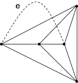
Figure 2: The graph $G$ (without the edge $e$) is planar $3$-connected. With $e$, the graph is $K_{5}$.

2.2 $2$-connected graphs

Quantum statistics on $2$-connected graphs is more complex, and depends on the decomposition of individual graphs into cycles and $3$-connected components (see Section 4.3). There may be multiple anyon and ${\mathbb{Z}}_{2}$ phases. But $2$-connected graphs share the following important property: their quantum statistics do not depend on the number of particles, and therefore can be regarded as a characteristic of the particle species. This property is important physically; it means that there is a building-up principle for increasing the number of particles in the system. This is described in detail in Section 7, where we show how to construct an $n$-particle Hamiltonian from a two-particle Hamiltonian. Interesting examples are also obtained by building $2$-connected graphs out of higher-connected components. Figure 3 shows a chain of identical non-planar 3-connected components. The links between components, represented by lines in figure 3, consist of at least two edges, so that resulting graph is $2$-connected. In this case, the quantum statistics is in fact independent of the number of particles, and may be determined by specifying exchange phases ($0$ or $\pi$) for each component in the chain. Thus, particles can act as bosons or fermions in different parts of the graph.

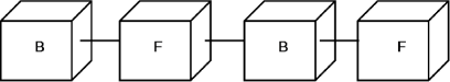
Figure 3: Linear chain of $3$-connected nonplanar components with alternating Bose and Fermi statistics.

2.3 $1$-connected graphs

Quantum statistics on graphs achieves its full complexity for 1-connected graphs, in which case it also depends on the number of particles $n$. A representative example, treated in detail in Section 6.1, is a star graph with $E$ edges, for which the number of anyon phases is given by

$$\beta_{n}^{E}={n+E-2\choose E-1}\left(E-2\right)-{n+E-2\choose E-2}+1,$$

and therefore depends on both $E$ and $n$.

2.4 Aharonov-Bohm phases

Configuration-space cycles on which one particle moves around a circuit $C$ while the others remain fixed play an important role in the analysis of quantum statistics which follows. We call these Aharonov-Bohm cycles, and the corresponding phases Aharonov-Bohm phases, because they correspond physically to magnetic fluxes threading $C$. In many-body systems, Aharonov-Bohm phases and quantum statistics phases can interact in interesting ways. In particular, Aharonov-Bohm phases can depend on the positions of the stationary particles. An example is shown in the two-particle octahedron graph (see figure 4), in which the Aharonov-Bohm phase associated with one particle going around the equator depends on whether the second particle is at the north or south pole. For $3$-connected non-planar graphs, it can be shown that Aharonov-Bohm phases are independent of the positions of the stationery particles. (The octahedron graph, despite appearances, is planar.)

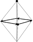
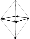
Figure 4: The Aharonov-Bohm phase for the equatorial cycle depends on whether the second particle is at the north or south pole.

3 Graph configuration spaces

Let $\Gamma$ be a metric connected simple graph with $V$ vertices and $E$ edges. In a metric graph edges correspond to finite closed intervals of $\mathbb{R}$. However, as we will be interested in the topology of the graph, the length of the edges will not play a role in the discussion. An undirected edge between vertices $v_{1}$ and $v_{2}$ will be denoted by $v_{1}\leftrightarrow v_{2}$. It will also be convenient to be able to label directed edges so $v_{1}\rightarrow v_{2}$ and $v_{2}\rightarrow v_{1}$ are the directed edges associated with $v_{1}\leftrightarrow v_{2}$. A path joining two vertices $v_{1}$ and $v_{m}$ is then specified by a sequence of $m-1$ directed edges, written $v_{1}\rightarrow v_{2}\rightarrow\dots\rightarrow v_{m}$.

We define the $n$-particle configuration space as the quotient space

$$C_{n}(\Gamma)=\left(\Gamma^{\times n}-\Delta\right)/S_{n},$$ (1)

where $S_{n}$ is the permutation group of $n$ elements and

$$\Delta=\{(x_{1},x_{2},\ldots,x_{n}):\exists_{i,j}\,x_{i}=x_{j}\},$$ (2)

is the set of coincident configurations. We are interested in the calculation of the first homology group, $H_{1}(C_{n}(\Gamma))$ of $C_{n}(\Gamma)$. The space $C_{n}(\Gamma)$ is not a cell complex. However, it is homotopy equivalent to the space $\mathcal{D}^{n}(\Gamma)$, which is a cell complex, defined below.

Recall that a cell complex $X$ is a nested sequence of topological spaces

$$X^{0}\subseteq X^{1}\subseteq\dots\subseteq X^{n},$$ (3)

where the $X^{k}$’s are the so-called $k$-skeletons defined as follows:

• The $0$ - skeleton $X^{0}$ is a finite set of points.

• For $\mathbb{N}\ni k>0$, the $k$ - skeleton $X^{k}$ is the result of attaching $k$ - dimensional balls $B_{k}=\{x\in\mathbb{R}^{k}\,:\,\|x\|\leq 1\}$ to $X^{k-1}$ by gluing maps

  $$\sigma:S^{k-1}\rightarrow X^{k-1},$$ (4)

  where $S^{k-1}$ is the unit-sphere $S^{k-1}=\{x\in\mathbb{R}^{k}\,:\,\|x\|=1\}$.

A $k$-cell is the interior of the ball $B_{k}$ attached to the $(k-1)$-skeleton $X^{k-1}$.

Every simple graph $\Gamma$ is naturally a cell complex; the vertices are $0$-cells (points) and edges are $1$-cells ($1$-dimensional balls whose boundaries are the $0$-cells). The product $\Gamma^{\times n}$ then naturally inherits a cell complex structure. The cells of $\Gamma^{n}$ are Cartesian products of cells of $\Gamma$. It is clear that the space $C_{n}(\Gamma)$ is not a cell complex as points belonging to $\Delta$ have been deleted. Following Abrams we define an $n$-particle combinatorial configuration space as

$$\mathcal{D}^{n}(\Gamma)=(\Gamma^{\times n}-\tilde{\Delta})/S_{n},$$ (5)

where $\tilde{\Delta}$ denotes all cells whose closure intersects with $\Delta$. The space $\mathcal{D}^{n}(\Gamma)$ possesses a natural cell complex structure. Moreover,

Theorem 3.1

Abrams For any graph $\Gamma$ with at least $n$ vertices, the inclusion $\mathcal{D}^{n}(\Gamma)\hookrightarrow C_{n}(\Gamma)$ is a homotopy equivalence iff the following hold:

1. Each path between distinct vertices of valence not equal to two passes through at least $n-1$ edges.

2. Each closed path in $\Gamma$ passes through at least $n+1$ edges.

Following Abrams ; FS05 we refer to a graph $\Gamma$ with properties 1 and 2 as sufficiently subdivided. For $n=2$ these conditions are automatically satisfied (provided $\Gamma$ is simple). Intuitively, they can be understood as follows:

1. In order to have homotopy equivalence between $\mathcal{D}^{n}(\Gamma)$ and $C_{n}(\Gamma)$, we need to be able to accommodate $n$ particles on every edge of graph $\Gamma$. This is done by introducing $n-2$ trivial vertices of degree $2$ to make a line subgraph between every adjacent pair of non-trivial vertices in the original graph $\Gamma$.

2. For every cycle there is at least one free (not occupied) vertex which enables the exchange of particles around this cycle.

For a sufficiently subdivided graph $\Gamma$ we can now effectively treat $\Gamma$ as a combinatorial graph where particles are accommodated at vertices and hop between adjacent unoccupied vertices along edges of $\Gamma$.

Using Theorem 3.1, the problem of finding $H_{1}(C_{n}(\Gamma))$ is reduced to the problem of computing $H_{1}(\mathcal{D}^{n}(\Gamma))$. In the next sections we show how to determine $H_{1}(\mathcal{D}^{n}(\Gamma))$ for an arbitrary simple graph $\Gamma$. Note, however, that by the structure theorem for finitely generated modules Nakahara

$$H_{1}(\mathcal{D}^{n}(\Gamma))=\mathbb{Z}^{k}\oplus T_{l}$$ (6)

where $T_{l}$ is the torsion, i.e.

$$T_{l}=\mathbb{Z}_{n_{1}}\oplus\ldots\oplus\mathbb{Z}_{n_{l}},$$ (7)

and $n_{i}|n_{i+1}$. In other words $H_{1}(\mathcal{D}^{n}(\Gamma))$ is determined by $k$ free parameters $\{\phi_{1},\ldots,\phi_{k}\}$ and $l$ discrete parameters $\{\psi_{1},\ldots,\psi_{l}\}$ such that for each $i\in\{1,\ldots l\}$

$$n_{i}\psi_{i}=0\,\,\mbox{mod}\,2\pi,\,\,n_{i}\in\mathbb{N}\,\,\,\>\mbox{and}\,\,n_{i}|n_{i+1}.$$ (8)

Taking into account their physical interpretation we will call the parameters $\phi$ and $\psi$ continuous and discrete phases respectively.

4 Two-particle quantum statistics

In this section we fully describe the first homology group $H_{1}(\mathcal{D}^{2}(\Gamma))$ for an arbitrary connected simple graph $\Gamma$. We start with three simple examples: a cycle, a Y-graph and a lasso. The $2$-particle discrete configuration space of the lasso reveals an important relation between the exchange phase on the Y-graph and on the cycle. Combining this relation with an ansatz for a perhaps over-complete spanning set of the cycle space of $\mathcal{D}^{2}(\Gamma)$ and some combinatorial properties of $k$-connected graphs, we give a formula for $H_{1}(\mathcal{D}^{2}(\Gamma))$. Our argument is divided into three parts; corresponding to $3$-, $2$- and $1$-connected graphs respectively.

Three examples

• Let $\Gamma$ be a triangle graph shown in figure 5(a). Its combinatorial configuration space $\mathcal{D}^{2}(\Gamma)$ is shown in figure 1(b). The cycle $(1,2)\rightarrow(1,3)\rightarrow(2,3)\rightarrow(1,2)$ is not contractible and hence $H_{1}(\mathcal{D}^{2}(\Gamma))=\mathbb{Z}$. In other words we have one free phase $\phi_{c}$ and no torsion.

Figure 5: (a) The triangle graph $\Gamma$ (b) The $2$-particle configuration space $\mathcal{D}^{2}(\Gamma)$

• Let $\Gamma$ be a Y-graph shown in figure 6(a). Its combinatorial configuration space $\mathcal{D}^{2}(\Gamma)$ is shown in figure 2(b). The cycle $(1,2)\rightarrow(1,3)\rightarrow(2,3)\rightarrow(3,4)\rightarrow(2,4)\rightarrow(1,4)\rightarrow(1,2)$ is not contractible and $H_{1}(\mathcal{D}^{2}(\Gamma))=\mathbb{Z}$. Hence we have one free phase $\phi_{Y}$ and no torsion.

Figure 6: (a) The Y-graph $\Gamma$ (b) The $2$-particle configuration space $\mathcal{D}^{2}(\Gamma)$

• Let $\Gamma$ be a lasso graph shown in figure 7(a). It is a combination of Y and triangle graphs. Its combinatorial configuration space $\mathcal{D}^{2}(\Gamma)$ is shown in figure 3(b). The shaded rectangle is a $2$-cell and hence the cycle $(1,3)\rightarrow(2,3)\rightarrow(2,4)\rightarrow(1,4)\rightarrow(1,3)$ is contractible. The cycle $(1,2)\rightarrow(1,3)\rightarrow(1,4)\rightarrow(1,2)$ corresponds to the situation when one particle is sitting at the vertex $1$ and the other moves along the cycle $c=2\rightarrow 3\rightarrow 4\rightarrow 2$ of $\Gamma$. We will call this cycle an Aharonov-Bohm cycle (AB-cycle) and denote its phase $\phi_{c,1}^{1}$. The cycle $(2,3)\rightarrow(3,4)\rightarrow(2,4)\rightarrow(2,3)$ represents the exchange of two particles around $c$. The corresponding phase will be denoted by $\phi_{c,2}$. Finally, for the cycle $(1,2)\rightarrow(1,3)\rightarrow(2,3)\rightarrow(3,4)\rightarrow(2,4)\rightarrow(1,4)\rightarrow(1,2)$, corresponding to exchange of two particles along a Y-graph, the phase is $\phi_{Y}$. There is no torsion in $H_{1}(\mathcal{D}^{2}(\Gamma))$. Moreover,

  $$\phi_{c,2}=\phi_{c,1}^{1}+\phi_{Y}.$$ (9)

  Notice that knowing $\phi_{Y}$ and the AB-phases determines the phases $\phi_{c,2}$. As we shall see, 9 plays an important role in relating Y-phases and AB-phases for general graphs.

Figure 7: (a) The lasso graph $\Gamma$ (b) The $2$-particle configuration space $\mathcal{D}^{2}(\Gamma)$

4.1 A spanning set of $H_{1}(\mathcal{D}^{2}(\Gamma))$

In order to proceed with the calculation of $H_{1}(\mathcal{D}^{2}(\Gamma))$ for arbitrary $\Gamma$ we need a spanning set of $H_{1}(\mathcal{D}^{2}(\Gamma))$. Before we give one, let us discuss the dependence of the AB-phase on the position of the second particle. Suppose there is a cycle $c$ in $\Gamma$ with two vertices $v_{1}$ and $v_{2}$ not on the cycle. We want to know the relation between $\phi_{c,1}^{v_{1}}$ and $\phi_{c,1}^{v_{2}}$. There are two possibilities to consider. The first is shown in figure 8(a) and represents the situation when there is a path $P_{v_{1},v_{2}}$ which joins $v_{1}$ and $v_{2}$ and is disjoint with $c$. In this case both AB-cycles are homotopy equivalent as they belong to the cylinder $c\times P_{v_{1},v_{2}}$. Therefore,

Fact 1

Assume there is a cycle $c$ in $\Gamma$ with two vertices $v_{1}$ and $v_{2}$ not on the cycle. Suppose there is a path $P_{v_{1},v_{2}}$ which joins $v_{1}$ and $v_{2}$ and is disjoint with $c$. Then $\phi_{c,1}^{v_{1}}=\phi_{c,1}^{v_{2}}$.

Assume now that there is a path joining $v_{1}$ and $v_{2}$ which passes through the cycle $c$ (see figure 8(b)). Using relation (9) we get

$$\phi_{c,2}=\phi_{c,1}^{v_{1}}+\phi_{Y_{1}},\,\,\,\,\phi_{c,2}=\phi_{c,1}^{v_{2}}+\phi_{Y_{2}},$$ (10)

and hence

$$\phi_{c,1}^{v_{1}}-\phi_{c,1}^{v_{2}}=\phi_{Y_{2}}-\phi_{Y_{1}}.$$ (11)

The relations between different AB-phases for a fixed cycle $c$ of $\Gamma$ are therefore encoded in the phases $\phi_{Y}$.

Figure 8: The dependence of the AB-phase for cycle $c$ on the position of the second particle when (a) there is a path between $v_{1}$ and $v_{2}$ disjoint with $c$, (b) every path joining $v_{1}$ and $v_{2}$ passes through $c$.

As we show in the appendix, a spanning set of $H_{1}(\mathcal{D}^{2}(\Gamma))$ is given by all Y and AB-cycles. Note that relations (9) and (11) reduce the number of relevant AB-cycles to one per independent cycle of $\Gamma$, i.e. to

$$\beta_{1}(\Gamma)=E-V+1,$$ (12)

cycles. As a result, we will use a spanning set (which in general is over-complete) containing the following:

1. All $2$-particle cycles corresponding to the exchanges on Y subgraphs of $\Gamma$. There can be dependencies between these cycles.

2. A set of $\beta_{1}(\Gamma)$ AB-cycles, one for each independent cycle in $\Gamma$.

Thus, $H_{1}(\mathcal{D}^{2}(\Gamma))=\mathbb{Z}^{\beta_{1}(\Gamma)}\oplus A$, where $A$ is determined by Y-cycles. Consequently, in order to determine $H_{1}(\mathcal{D}^{2}(\Gamma))$ one has to study the relations between Y-cycles.

4.2 $3$-connected graphs

In this section we determine $H_{1}(\mathcal{D}^{2}(\Gamma))$ for $3$-connected graphs. Let $\Gamma$ be a connected graph. We define an $m$-separation of $\Gamma$ tutte01 , where $m$ is a positive integer, as an ordered pair $(\Gamma_{1},\Gamma_{2})$ of subgraphs of $\Gamma$ such that

1. The union $\Gamma_{1}\cup\Gamma_{2}=\Gamma$.

2. $\Gamma_{1}$ and $\Gamma_{2}$ are edge-disjoint and have exactly $m$ common vertices, $V_{m}=\{v_{1},\ldots,v_{m}\}$.

3. $\Gamma_{1}$ and $\Gamma_{2}$ have each a vertex not belonging to the other.

It is customary to say that the $V_{m}$ separates vertices of $\Gamma_{1}$ and $\Gamma_{2}$ different from $V_{m}$.

Definition 1

A connected graph $\Gamma$ is $n$-connected iff it has no $m$-separation for any $m<n$.

The following theorem of Menger tutte01 gives an additional insight into graph connectivity:

Theorem 4.1

For an $n$-connected graph $\Gamma$ there are at least $n$ internally disjoint paths between any pair of vertices.

The basic examples of $3$-connected graphs are wheel graphs. A wheel graph $W^{n}$ of order $n$ consists of a cycle with $n$ vertices and a single additional vertex which is connected to each vertex of the cycle by an edge. Following Tutte tutte01 we denote the middle vertex by $h$ and call it the hub, and the cycle that does not include $h$ by $R$ and call it the rim. The edges connecting the hub to the rim will be called spokes. The importance of wheels in the theory of $3$-connected graphs follows from the following theorem;

Theorem 4.2

(Wheel theorem tutte01 ) Let $\Gamma$ be a simple $3$-connected graph different from a wheel. Then for some edge $e\in E(\Gamma)$ either $\Gamma\setminus e$ or $\Gamma/e$ is simple and $3$-connected.

Here $\Gamma\setminus e$ is constructed from $\Gamma$ by removing the edge $e$, and $\Gamma/e$ is obtained by contracting edge $e$ and identifying its vertices. These two operations will be called edge removal and edge contraction. The inverses will be called edge addition and vertex expansion. Note that that vertex expansion requires specifying which edges are connected to which vertices after expansion. As we deal with $3$-connected graphs we will apply the vertex expansion only to vertices of degree at least four and split the edges between new vertices in a such way that they are at least $3$-valent.

As a direct corollary of Theorem 4.2 any simple $3$-connected graph can be constructed in a finite number of steps starting from a wheel graph $W^{k}$, for some $k$

$$W_{k}=\Gamma_{0}\mapsto\Gamma_{1}\mapsto\ldots\mapsto\Gamma_{n-1}\mapsto\Gamma_{n}=\Gamma$$

where $\Gamma_{i}$ is constructed from $\Gamma_{i-1}$ by either

1. Adding an edge between non-adjacent vertices or

2. Expanding at the vertex of the valency at least four.

Moreover, each $\Gamma_{i}$ is simple and $3$-connected. In order to prove inductively some feature of a $3$-connected graph it is therefore enough to show it for an arbitrary wheel and consider what happens when an edge between two non-adjacent vertices is added or a vertex of valency at least four is expanded.

Lemma 1

For wheel graphs $W^{n}$ all phases $\phi_{Y}$ are equal up to the sign.

Proof

The Y subgraphs of $W^{n}$ can be divided into two groups: (i) the central vertex of Y is on the rim (ii) the center vertex of Y is the hub. For (i) let $v_{1}$ and $v_{2}$ be two adjacent vertices belonging to the rim, $R$. Let $Y_{v_{1}}$ and $Y_{v_{2}}$ be the corresponding Y-graphs whose central vertices are $v_{1}$ and $v_{2}$ respectively and one edge is a spoke. Evidently two edges of $Y_{v_{1}}$ and $Y_{v_{2}}$ belong to the same triangle cycle, $C$ i.e the one spanned by $v_{1}$, $v_{2}$ and the hub (see figure 9(a)). Moreover, $b_{1}$ is connected to $b_{2}$ by a path which is disjoint with $C$. Using Fact 1 and relation (11) we get $\phi_{Y_{v_{1}}}=\phi_{Y_{v_{2}}}$. Repeating this reasoning we obtain that all $\phi_{Y_{v_{i}}}$, with $v_{i}$ belonging to the rim are equal (perhaps up to the sign). We are left with the Y-graphs whose central vertex is the hub. Similarly (see figure 9(b)) we take a cycle, $C$, with two edges belonging to the chosen Y. But there is always a Y-graph with two edges belonging to $C$ and center to the rim. Therefore, by Fact 1 and relation (11) the phase on the Y subgraph whose center vertex is the hub is the same as on the Y subgraphs whose center vertex is on the rim.∎

Figure 9: (a) Graphs $Y_{v_{1}}$ and $Y_{v_{2}}$(b) Graphs $Y_{h}$ and $Y_{v_{2}}$

Lemma 2

For $3$-connected simple graphs all phases $\phi_{Y}$ are equal up to the sign.

Proof

We prove by induction. By Lemma 1 the statement is true for all wheel graphs.

Adding an edge: Assume that $v_{1}$ and $v_{2}$ are non-adjacent vertices of the $3$-connected graph $\Gamma$ and all $\phi_{Y}$ phases are equal (up to the sign). By adding an edge between the vertices $v_{1}$ and $v_{2}$ we do not change the relations between the $\phi_{Y}$ phases of $\Gamma$. However, the graph $\Gamma\cup e$ contains new Y-graphs, whose middle vertices are $v_{1}$ or $v_{2}$ and one of the edges is $e$. We need to show that the phase $\phi_{Y}$ for these new Y’s is the same as on the old ones. Let $\{e,f_{1},f_{2}\}$ be such a Y-graph (see figure 10(a)). Let $\alpha_{1}$ and $\alpha_{2}$ be endpoints of $f_{1}$ and $f_{2}$. By $3$-connectedness, there is a path between $\alpha_{1}$ and $\alpha_{2}$ which does not contain $v_{1}$ or $v_{2}$. In this way we obtain a cycle $C$, as shown in figure 10(a). Again by $3$-connectedness, there is a path $P$ from $v_{2}$ to a vertex $\beta$ in $C$. Let $Y^{\prime}$ be the Y-graph with $\beta$ as its centre and edges along $C$ and $P$, as shown in figure 10(a). Then $Y^{\prime}$ belongs to $\Gamma$. Applying Fact 1 and relation (11) to the cycle $C$ and the two Y-graphs discussed, the result follows.

Vertex expansion: Let $\Gamma$ be a $3$-connected simple graph and let $v$ be a vertex of degree at least four. Let $\tilde{\Gamma}$ be a graph derived from $\Gamma$ by expanding at the vertex $v$ and assume that the new vertices, $v_{1}$ and $v_{2}$, are at least $3$-valent. These assumptions are necessary for $\tilde{\Gamma}$ to be $3$-connected tutte01 . Note that $\Gamma$ and $\tilde{\Gamma}$ have the same number of independent cycles. Moreover, by splitting at the vertex $v$ we do not change the relations between the $\phi_{Y}$ phases of $\Gamma$. This is simply because if the equality of some of the $\phi_{Y}$ phases required a cycle passing through $v$, one can now use the cycle with one more edge passing through $v_{1}$ and $v_{2}$ in $\tilde{\Gamma}$. The graph $\tilde{\Gamma}$ contains new Y-graphs, whose middle vertices are $v_{1}$ or $v_{2}$ and one of the edges is $e=v_{1}\leftrightarrow v_{2}$. We need to show that the phase $\phi_{Y}$ on these new Ys is the same as on the old ones. Let $\{e,f_{1},f_{2}\}$ be such a graph and let $\alpha_{1}$ and $\alpha_{2}$ be endpoints of $f_{1}$ and $f_{2}$. By $3$-connectedness, there is a path between $\alpha_{1}$ and $\alpha_{2}$ which does not contain $v_{1}$ or $v_{2}$. In this way we obtain a cycle $C$, as shown in figure 10(b). Again by $3$-connectedness, there is a path $P$ from $v_{2}$ to a vertex $\beta$ in $C$. Let $Y^{\prime}$ be the Y-graph with $\beta$ as its centre and edges along $C$ and $P$, as shown in figure 10(b). Then $Y^{\prime}$ belongs to $\Gamma$. Applying Fact 1 and relation (11) to the cycle $C$ and the two Y-graphs discussed, the result follows.∎

Figure 10: (a) Adding an edge (b) Expanding at the vertex.

Theorem 4.3

For a $3$-connected simple graph, $H_{1}(\mathcal{D}^{2}(\Gamma))=\mathbb{Z}^{\beta_{1}(\Gamma)}\oplus A$, where $A=\mathbb{Z}_{2}$ for non-planar graphs and $A=\mathbb{Z}$ for planar graphs.

Proof

By Lemmas 1 and 2 we only need to determine the phase $\phi_{Y}$. It was shown in JHJKJR that for the graphs $K_{5}$ and $K_{3,3}$ $H_{1}(\mathcal{D}^{2}(\Gamma))=\mathbb{Z}^{\beta_{1}(\Gamma)}\oplus\mathbb{Z}_{2}$. Therefore the phase $\phi_{Y}=0$ or $\pi$. By Kuratowski’s theorem Kuratowski30 every non-planar graph contains a subgraph which is isomorphic to $K_{5}$ or $K_{3,3}$. This proves the statement for non-planar graphs. For planar graphs we have the anyon phase and hence $A=\mathbb{Z}$. This is because for planar graphs, one can introduce anyon phases by drawing the graph in the plane and integrating the anyon vector potential $\frac{\alpha}{2\pi}\hat{z}\times\frac{r_{1}-r_{2}}{|r_{1}-r_{2}|^{2}}$ along the edges of the two-particle graph, where $r_{1}$ and $r_{2}$ are the positions of the particles.∎

Finally, note that as a direct consequence of relation (11) and Theorem 4.3, AB-phases for $3$-connected nonplanar graphs are independent of the positions of stationary particles. This is not necessarily the case for $3$-connected planar graphs, as $\phi_{Y}$ phases are equal only up to the sign.

4.3 $2$-connected graphs

In this subsection we discuss $2$-connected graphs. First, by considering a simple example we show that in contrast to $3$-connected graphs it is possible to have more than one $\phi_{Y}$ phase. Using a decomposition procedure of a $2$-connected graph into $3$-connected graphs and topological cycles we provide the formula for $H_{1}(\mathcal{D}^{2}(\Gamma))$.

Figure 11: (a) An example of a $2$-connected graph, (b) the components of the $2$-cut $\{x,y\}$, (c) the marked components.

Example 1

Let us consider graph $\Gamma$ shown in figure 11(a). Since vertices $v_{1}$ and $v_{4}$ are $2$-valent, $\Gamma$ is not $3$-connected. It is however $2$-connected. Note that $\beta_{1}(\Gamma)=4$ and that there are six Y-graphs, with middle vertices $v_{2}$, $v_{3}$, $v_{5}$, $v_{6}$, $x$ and $y$ respectively. Using Fact 1 and relation (11) we verify that

$$\phi_{Y_{v_{2}}}=\phi_{Y_{v_{6}}},\,\,\phi_{Y_{v_{3}}}=\phi_{Y_{v_{5}}},\,\,\phi_{Y_{x}}=\phi_{Y_{y}}.$$ (13)

It is also straightforward to show that the phases $\phi_{Y_{v_{2}}}$, $\phi_{Y_{v_{3}}}$ and $\phi_{Y_{x}}$ are independent. Therefore we have three independent $\phi_{Y}$ phases and four AB-phases, and so

$$H_{1}(\mathcal{D}^{2}(\Gamma))=\mathbb{Z}^{6}.$$ (14)

Vertices $\{x,y\}$ constitute a $2$-vertex cut of $\Gamma$, i.e. after their deletion $\Gamma$ splits into three connected components $\Gamma_{1}$, $\Gamma_{2}$, $\Gamma_{3}$ (see figure 11(b)). They are no longer $2$-connected. Moreover, for example, the two Y-subgraphs $Y_{v_{2}}$ and $Y_{v_{6}}$ for which $\phi_{Y_{v_{2}}}=\phi_{Y_{v_{6}}}$ in $\Gamma$ no longer satisfy this condition in $\Gamma_{1}$, i.e. $\phi_{Y_{v_{2}}}\neq\phi_{Y_{v_{6}}}$ in $\Gamma_{1}$. This is because the AB-phases $\phi_{C_{1},1}^{x}$ and $\phi_{C_{1},1}^{y}$ are not equal. To make components $\Gamma_{i}$ $2$-connected and at the same time keep the correct relations between $\phi_{Y_{v_{i}}}$, it is enough to add to each component $\Gamma_{i}$ an additional edge between vertices $x$ and $y$ (see figure 11(c)). The resulting graphs, which we call the marked components and denote by $\tilde{\Gamma}_{i}$ KP11 , are $2$-connected and the relations between the Y-graphs in each $\tilde{\Gamma}_{i}$ are the same as in $\Gamma$. The union of the three marked components has, however, $\beta_{1}(\Gamma)+1$ independent cycles. On the other hand, by splitting $\Gamma$ into marked components the Y-cycles $Y_{x}$ and $Y_{y}$ have been lost. Since $\phi_{Y_{x}}=\phi_{Y_{y}}$ we have lost one $\phi_{Y}$ phase. Summing up we can write $H_{1}(\mathcal{D}^{2}(\Gamma))\oplus\mathbb{Z}=\bigoplus_{i=1}^{3}H_{1}(\mathcal{D}^{2}(\tilde{\Gamma}_{i}))\oplus\mathbb{Z}$.

2-vertex cut for an arbitrary $2$-connected graph $\Gamma$

In figure 12(a) a more general $2$-vertex cut is shown together with components $\Gamma_{i}$. It is easy to see that the marked components $\tilde{\Gamma}_{i}$ are $2$-connected and the relations between the $\phi_{Y}$ phases in each $\tilde{\Gamma}_{i}$ are the same as in $\Gamma$. Let $\mu(x,y)$ be the number of $\tilde{\Gamma}_{i}$ components into which $\Gamma$ splits after removal of vertices $x$ and $y$. By Euler’s formula the union $\{\tilde{\Gamma}_{i}\}_{i=1}^{\mu(x,y)}$ of $\mu(x,y)$ marked components has

$$\beta=\#\mathrm{edges}-\#\mathrm{vertices}+\mu(x,y)$$

$$=E(\Gamma)+\mu(x,y)-\left(V(\Gamma)+2(\mu(x,y)-1)\right)+\mu(x,y)$$

$$=E(\Gamma)-V(\Gamma)+2=\beta_{1}(\Gamma)+1,$$ (15)

independent cycles. By splitting $\Gamma$ into the marked components we possibly lose $\phi_{Y}$ phases corresponding to the Y-graphs with the middle vertex $x$ or $y$. However

1. If three edges of a Y-graph are connected to the same component we do not lose $\phi_{Y}$.

2. If two edges of a Y-graph are connected to the same component we do not lose $\phi_{Y}$. This can be understood by looking at figure 12(b). The phase of the dashed Y-graph which is lost is the same as the phase of the dotted Y-graph inside $\Gamma_{2}$.

Hence the $\phi_{Y}$ phases we lose correspond to the Y-graphs for which each edge is connected to a different component. First we want to show that any two Y-graphs with the central vertex $x$ (or $y$) whose edges are connected to three fixed components have the same phase. It is enough to show this for Y-graphs which share the same center and two edges. Let us consider two such Y-graphs (see figure 12(c) - the dashed egdes are common for both Y-graphs). Let $\alpha_{1}$ and $\alpha_{2}$ be endpoints of edges which are not shared by both Y-graphs. Since there is a path between $\alpha_{1}$ and $\alpha_{2}$ in $\Gamma_{2}$ and paths $P_{a_{1},a_{2}}$, $P_{b_{1},b_{2}}$ in $\Gamma_{1}$ and $\Gamma_{3}$ respectively we can apply Fact 1 and relation (11) to the cycle $x\rightarrow a_{1}\cup P_{a_{1},a_{2}}\cup a_{2}\rightarrow y\rightarrow b_{2}\cup P_{b_{1},b_{2}}\cup b_{2}\rightarrow x$ and the two considered Y-graphs obtaining equality of the two respective $\phi_{Y}$ phases. Therefore, the choice of three components gives only one $\phi_{Y}$ phase. Moreover, note that after choosing three components the phase for the Y-graph with the middle vertex $x$ is the same as for the Y-graph with the middle vertex $y$ (see figure 12(d) where the considered Y-graphs are denoted by dashed and dotted lines). This is once again due to Fact 1 and relation (11) applied to the cycle $x\rightarrow a_{1}\cup P_{a_{1},a_{2}}\cup a_{2}\rightarrow y\rightarrow\alpha_{2}\cup P_{\alpha_{1},\alpha_{2}}\cup\alpha_{2}\rightarrow x$ and the two considered Y-graphs. Summing up, the number of phases we lose when splitting $\Gamma$ into $\mu(x,y)$ marked components, $N_{2}(x,y)$, is equal to the number of independent Y-graphs in the star graph with $\mu(x,y)$ edges. This can be calculated (see for example JHJKJR ) to be $N_{2}(x,y)=\frac{1}{2}\left(\mu(x,y)-2\right)\left(\mu(x,y)-1\right)$. Hence

$$H_{1}(\mathcal{D}^{2}(\Gamma))=\bigoplus_{i=1}^{\mu(x,y)}H_{1}(\mathcal{D}^{2}(\tilde{\Gamma}_{i}))\oplus\mathbb{Z}^{N_{2}(x,y)-1}.$$ (16)

Note that the $-1$ in the exponent here is to get rid of the additional AB-phase stemming from the calculation (15).

Figure 12: (a) 2-vertex cut of $\Gamma$ (b) $Y_{x}$ with two edges connected to $\Gamma_{2}$ (c) two Y-cycles with three edges in three different components (d) the equality of $\phi_{Y_{x}}$ and $\phi_{Y_{y}}$

Finally, it is known in graph theory that by the repeated application of the above decomposition procedure the resulting marked components are either topological cycles or $3$-connected graphs tutte01 . Let $n$ be the number of $2$-vertex cuts which is needed to get such a decomposition, $N_{2}=\sum_{\{x_{i},y_{i}\}}N_{2}(x_{i},y_{i})$, $N_{3}$ the number of planar $3$-connected components, $N_{3}^{\prime}$ the number of non-planar $3$-connected components and $N_{3}^{{}^{\prime\prime}}$ the number of the topological cycles. Let $\mu=N_{3}+N_{3}^{{}^{\prime}}+N_{3}^{{}^{\prime\prime}}$. Then

$$H_{1}(\mathcal{D}^{2}(\Gamma))=\bigoplus_{i=1}^{\mu}H_{1}(\mathcal{D}^{2}(\tilde{\Gamma}_{i}))\oplus\mathbb{Z}^{N_{2}-n},$$ (17)

where

$$H_{1}(\mathcal{D}^{2}(\tilde{\Gamma}_{i}))=\mathbb{Z}^{\beta_{1}(\tilde{\Gamma}_{i})}\oplus\mathbb{Z},\,\,\,\tilde{\Gamma}_{i}-\mathrm{planar}$$ (18)

$$H_{1}(\mathcal{D}^{2}(\tilde{\Gamma}_{i}))=\mathbb{Z}^{\beta_{1}(\tilde{\Gamma}_{i})}\oplus\mathbb{Z}_{2},\,\,\,\tilde{\Gamma}_{i}-\mathrm{nonplanar}$$

$$H_{1}(\mathcal{D}^{2}(\tilde{\Gamma}_{i}))=\mathbb{Z},\,\,\,\tilde{\Gamma}_{i}-\mathrm{topological}\,\,\mathrm{cycle}$$

Note that $\sum_{i}\beta_{1}(\tilde{\Gamma}_{i})+N_{3}^{{}^{\prime\prime}}=\beta_{1}(\Gamma)+n$ and therefore

$$H_{1}(\mathcal{D}^{2}(\Gamma))=\mathbb{Z}^{\beta_{1}(\Gamma)+N_{2}+N_{3}}\oplus\mathbb{Z}_{2}^{N_{3}^{\prime}}.$$ (19)

4.4 $1$-connected graphs

In this subsection we focus on $1$-connected graphs. Assume that $\Gamma$ is $1$-connected but not $2$-connected. There exists a vertex $v\in V(\Gamma)$ such that after its deletion $\Gamma$ splits into at least two connected components. Denote by $\Gamma_{1},\ldots,\Gamma_{\mu(v)}$ these components. Assume that $\Gamma_{i}$ is attached to $v$ by $E_{i}$ edges and put $\nu(v)=\sum_{i}E_{i}$, so that $\nu(v)$ is the total number of edges at $v$. By Euler’s formula the union of components $\{\Gamma_{i}\}_{i=1}^{{\mu(v)}}$ has

$$E(\Gamma)-\left(V(\Gamma)+\mu(v)-1\right)+\mu(v)=\beta_{1}(\Gamma),$$ (20)

independent cycles, hence the number of independent cycles does not change compared to $\Gamma$. Moreover, the phases $\phi_{Y}$ inside each of the components are the same as in $\Gamma$. Note, however, that by splitting we lose Y-graphs whose three edges do not belong to one fixed component $\Gamma_{i}$. Consequently, there are two cases to consider:

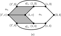
Figure 13: (a)Two edges of $Y$ are attached to $\Gamma_{v,3}$ while the third one to $\Gamma_{v,1}$ (b) Each edge of Y is attached to a different component (c) Y-graphs with two edges in the same component (d) Two Y-graphs (d) The relevant part of $2$-particle configuration space of (d)

1. Two edges of the Y-graph are attached to one component, for example $\Gamma_{v,3}$, while the third one is attached to another component, $\Gamma_{v,1}$. We claim that the phase $\phi_{Y}$ does not depend on the choice of the third edge, provided it is attached to $\Gamma_{v,1}$. To see this consider two Y-graphs, $Y_{1}$ and $Y_{2}$ shown in figure 13(a). Since vertices $\alpha_{1}$ and $\alpha_{2}$ are connected by a path, by Fact 1 $\phi_{C,1}^{\alpha_{1}}=\phi_{C,1}^{\alpha_{2}}$. Next, relation (11) applied to cycle $C$ and the two considered Y graphs gives $\phi_{Y_{1}}=\phi_{Y_{2}}$.
   

   After choosing one edge of Y in component $\Gamma_{v,1}$ (by the above argument it does not matter which), we can choose the two other edges in $\Gamma_{v,3}$ in $E_{3}\choose{2}$ ways. Therefore, a priori, we have $E_{3}\choose{2}$ Y-graphs to consider. There are, however, relations between them. In order to find the relevant relations consider the graph shown in figure 13(c). We are interested in Y-graphs with one edge given by $\alpha_{1}\leftrightarrow v$ (dashed line) and two edges joining $v$ to vertices in $\Gamma_{v,3}$, say $j$ and $k$. Each such Y-graph determines a cycle $c$ in $\Gamma_{v,3}$ containing vertices $v$, $j$ and $k$ (since $\Gamma_{v,3}$ is connected). We have that

   $$\phi_{c,2}=\phi_{c,1}^{\alpha_{1}}+\phi_{Y}.$$ (21)

   Therefore, the $E_{3}\choose{2}$ $Y$-phases under consideration are determined by the AB- and two-particle phases, $\phi_{c,2}$ and $\phi_{c,1}^{\alpha_{1}}$, of the associated cycles $c$. These cycles may be expressed as linear combinations of a basis of $E_{3}-1$ cycles, denoted $c_{1},\ldots,c_{E_{3}-1}$, as in figure 13(c). It is clear that if $c=\sum_{i=1}^{E_{3}}r_{i}c_{i}$, then

   $$\phi_{c,1}^{\alpha_{1}}=\sum_{i=1}^{E_{3}-1}r_{i}\phi_{c_{i},1}^{\alpha_{1}},\quad\,\,\,\phi_{c,2}=\sum_{i=1}^{E_{3}-1}r_{i}\phi_{c_{i},2}.$$ (22)

   Thus, the $Y$-phases under consideration may be expressed in terms of the $2(E_{3}-1)$ phases $\phi_{c_{i},2}$ and $\phi_{c_{i},1}^{\alpha_{1}}$.
   

   Let $Y_{i}$ be the $Y$-graph which determines the cycle $c_{i}$. We may turn the preceding argument around; from (21), the AB-phase $\phi_{c_{i},1}^{\alpha_{1}}$ can be expressed in terms of $\phi_{Y_{i}}$ and $\phi_{c_{i},2}$. Combining the preceding observations, we deduce that the $\binom{E_{3}}{2}$ Y-phases lost when the vertex $v$ is removed may be expressed in terms of the phases $\phi_{c_{i},2}$ and $\phi_{Y_{i}}$. The phases $\phi_{c_{i},2}$ remain when $v$ is removed. It follows that phases $\phi_{Y_{i}}$ suffice to determine all of the lost phases, so that the number of independent $Y$-phases lost is $E_{3}-1$. Repeating this argument for each component, the total number of Y-phases lost is $\sum_{i=1}^{\mu(v)}(E_{i}-1)(\mu(v)-1)=(\mu(v)-1)(\nu(v)-\mu(v))$.
   

2. Each edge of Y is attached to a different component. We will show now that once three different components have been chosen it does not matter which of the edges attaching $\Gamma_{v,i}$ to $v$ we choose. To see this let us consider two Y-graphs shown in figure 13(b). The first one consists of the three dashed edges and the second of two dashed edges attached to $\Gamma_{v,1}$ and $\Gamma_{v,2}$ respectively and the dotted edged attached to $\Gamma_{v,3}$. We will show that the phase corresponding to Y-graph $\{1^{\prime}\leftrightarrow v,\,v\leftrightarrow 3,\,v\leftrightarrow 4\}$ is determined by the phase corresponding to Y-graph $\{1\leftrightarrow v,\,v\leftrightarrow 3,\,v\leftrightarrow 4\}$ (see figure 13(d)) and phases added in the previously considered step. It is clear by figure 13(e) that

   $$\phi_{Y_{2}}=\phi_{Y_{1}}+\phi_{c,1}^{3}+\phi_{c,1}^{4}.$$ (23)

   But phases $\phi_{c,1}^{3}$ and $\phi_{c,1}^{4}$ are known, as they have been added in the previous step. Thus, the number of the independent Y-phases we lose is equal to the number of independent Y-cycles in the two-particle configuration space of the star graph with $\mu(v)$ edges, that is, $(\mu(v)-1)(\mu(v)-2)/2$.

Summing up we can write

$$H_{1}(\mathcal{D}^{2}(\Gamma))=\bigoplus_{i=1}^{\mu(v)}H_{1}(\mathcal{D}^{2}(\Gamma_{v,i}))\oplus\mathbb{Z}^{N_{1}(v)},$$ (24)

where $N_{1}(v)=(\mu(v)-1)(\mu(v)-2)/{2}+(\mu(v)-1)(\nu(v)-\mu(v))$. It is known in graph theory tutte01 that by the repeated application of the above decomposition procedure the resulting components become finally $2$-connected graphs. Let $v_{1},\ldots,v_{l}$ be the set of cut vertices such that components $\Gamma_{v_{i},k}$ are $2$-connected. Making use of formula (19) we can write

$$H_{1}(\mathcal{D}^{2}(\Gamma))=\mathbb{Z}^{\beta(\Gamma)+N_{1}+N_{2}+N_{3}}\oplus\mathbb{Z}_{2}^{N_{3}^{\prime}},$$ (25)

where $N_{1}=\sum_{i}N_{1}(v_{i})$.

5 n-particle statistics for $2$-connected graphs

Having discussed $2$-particle configuration spaces, we switch to the $n$-particle case, $\mathcal{D}^{n}(\Gamma)$, where $n>2$. We proceed in a similar manner to the previous section. First we give a spanning set of $H_{1}(\mathcal{D}^{n}(\Gamma))$. Next we show that if $\Gamma$ is $2$-connected the first homology group stabilizes with respect to $n$, that is, $H_{1}(\mathcal{D}^{n}(\Gamma))=H_{1}(\mathcal{D}^{2}(\Gamma))$. Making use of formula (25)

$$H_{1}(\mathcal{D}^{n}(\Gamma))=\mathbb{Z}^{\beta(\Gamma)+N_{2}+N_{3}}\oplus\mathbb{Z}_{2}^{N_{3}^{\prime}}.$$

5.1 A spanning set of $H_{1}(\mathcal{D}^{n}(\Gamma))$

In order to calculate $H_{1}(\mathcal{D}^{n}(\Gamma))$ we first need to subdivide the edges of $\Gamma$ appropriately. By Theorem 3.1 each edge of $\Gamma$ must be able to accommodate $n$ particles and each cycle needs to have at least $n+1$ vertices, that is, $\Gamma$ needs to be sufficiently subdivided. Before we specify a spanning set of $H_{1}(\mathcal{D}^{n}(\Gamma))$ we first discuss two interesting aspects of this space. The first one concerns the relation between the exchange phase of $k$ particles, $k\leq n$ on the cycle $C$ of the lasso graph and its $\phi_{Y}$ phases (see Lemma 3 ). The second gives the relation between the AB-phases for fixed cycle $c$ of $\Gamma$ and the different possible positions of the $n-1$ stationary particles.

Lemma 3

The exchange phase, $\phi_{C,n}$, of $n$ particles on the cycle $c$ of the lasso graph is the sum of the exchange phase, $\phi_{C,n-1}^{1}$, of $n-1$ particles on the cycle $C$ with the last particle sitting at the vertex not belonging to $C$, e.g. vertex $1$, and the phase $\phi_{Y}$ associated with the exchange of two particles on the $Y$ subgraph with $n-2$ particles placed in the vertices $v_{1},\ldots,v_{n-2}$ of $C$ not belonging to the Y

$$\phi_{C,n}=\phi_{C,n-1}^{1}+\phi_{Y}^{v_{1},\ldots,v_{n-2}}.$$

Proof

By (9) the above lemma is true for $n=2$. For the proof in the general case it is enough to consider the lasso graphs with $3$ and $4$ particles shown in figures 14(a) and 14(b). It is easy to see that they are indeed sufficiently subdivided. The Y-graphs we consider are $\{2\leftrightarrow 3,\,3\leftrightarrow 4,\,3\leftrightarrow 6\}$ and $\{3\leftrightarrow 4,\,4\leftrightarrow 5,4\leftrightarrow 8\}$ respectively. The relevant parts of the $3$ and $4$-particle configuration spaces are shown in figures 15(a) and 15(b). The statement follows immediately from these figures.∎

Figure 14: The subdivided lasso for (a) $3$ particles, (b) $4$ particles.

Figure 15: The relevant parts of the configurations spaces for the lasso graphs with (a) $3$ particles: $\phi_{C,3}=\phi^{2}_{C,2}+\phi^{5}_{Y}$, (b) $4$ particles: $\phi_{C,4}=\phi^{3}_{C,3}+\phi^{6,7}_{Y}$.

By repeated application of Lemma 3 we see that $\phi_{C,n}$ can be expressed as a sum of an AB-phase and the Y-phases corresponding to different positions of $n-2$ particles. For example in the case of the graphs from figure 14(a) and 14(b) we get

$$\phi_{C,3}=\phi_{Y}^{5}+\phi_{C,2}^{2}=\phi_{Y}^{5}+\phi_{Y}^{1}+\phi_{C,1}^{1,2}\,,$$

$$\phi_{C,4}=\phi_{Y}^{6,7}+\phi_{C,3}^{3}=\phi_{Y}^{6,7}+\phi_{C,3}^{1}=\phi_{Y}^{6,7}+\phi_{Y}^{1,6}+\phi_{Y}^{1,2}+\phi_{C,1}^{1,2,3}\,.$$

Aharonov-Bhom phases

Assume now that we have $n$ particles on $\Gamma$. Let $C$ be a cycle of $\Gamma$ and $e_{1}$ and $e_{2}$ two sufficiently subdivided edges attached to $C$ (see figure 16(a)). We denote by $\phi_{C,1}^{k_{1},k_{2}}$ the AB-phase corresponding to the situation where one particle goes around the cycle $C$ while $k_{1}$ particles are in the edge $e_{1}$ and $k_{2}$ particles are in the edge $e_{2}$, $k_{1}+k_{2}=n-1$. For each distribution $(k_{1},k_{2})$ of the $n-1$ particles between the edges $e_{1}$ and $e_{2}$ we get a (possibly) different AB-cycle and AB-phase in $\mathcal{D}^{n}(\Gamma)$. We want to know how they are related. To this end notice that

$$\phi_{C,2}^{k_{1},k_{2}}=\phi_{C,1}^{k_{1}+1,k_{2}}+\phi_{Y_{1}}^{k_{1},k_{2}},\,\,\,\,\phi_{C,2}^{k_{1},k_{2}}=\phi_{C,1}^{k_{1},k_{2}+1}+\phi_{Y_{2}}^{k_{1},k_{2}},$$ (26)

and hence

$$\phi_{C,1}^{k_{1}+1,k_{2}}-\phi_{C,1}^{k_{1},k_{2}+1}=\phi_{Y_{2}}^{k_{1},k_{2}}-\phi_{Y_{1}}^{k_{1},k_{2}}.$$ (27)

The relations between different AB-phases for a fixed cycle $C$ of $\Gamma$ are therefore encoded in the $2$-particle phases $\phi_{Y}$, albeit these phases can depend on the positions of the remaining $n-2$ particles.

Figure 16: (a) The relation between AB-phases, (b) the stabilization of the first homology group.

A spanning set of $H_{1}(\mathcal{(}D)^{n}(\Gamma))$ is by the following (see appendix for proof):

1. All $2$-particle cycles corresponding to the exchange of two particles on the Y subgraph while $n-2$ particles are at vertices not belonging to the considered Y-graph. In general the phases $\phi_{Y}$ depend on the position of the remaining $n-2$ particles.

2. The set of $\beta_{1}(\Gamma)$ AB-cycles, where $\beta_{1}(\Gamma)$ is the number of the independent cycles of $\Gamma$.

Theorem 5.1

For a $2$-connected graph $\Gamma$ the the first homology group stabilizes with respect to the number of particles, i.e. $H_{1}(\mathcal{D}^{n}(\Gamma))=H_{1}(\mathcal{D}^{2}(\Gamma))$.

Proof

Using our spanning set it enough to show that phases on the Y-cycles do not depend on the position of the remaining $n-2$ particles. Notice that if any pair of the vertices not belonging to the chosen Y-graph is connected by a path then clearly the corresponding Y-phases have this property. Since the graph $\Gamma$ is $2$-connected it remains at least $1$-connected after removal of a vertex. Removing the central vertex of the Y (see figure 16(b)), the theorem follows.∎

6 N-particle statistics on $1$-connected graphs

By Theorem 5.1, in order to fully characterize the first homology group of $\mathcal{D}^{n}(\Gamma)$ for an arbitrary graph $\Gamma$ we are left to calculate $H_{1}(\mathcal{D}^{n}(\Gamma))$ for graphs which are 1-connected but not 2-connected. This is achieved by considering $n$-particle star and fan graphs.

6.1 Star graphs

In the following we consider a particular family of $1$-connected graphs, namely the star graphs $S_{E}$ with $E$ edges (see figure 17(a)). Our aim is to provide a formula for the dimension of the first homology group, $\beta_{n}^{E}$, of the $n$-particle configuration space $\mathcal{D}^{n}(S_{E})$. Let us recall that a graph $\Gamma$ is $1$-connected iff after deletion of one vertex it splits into at least two connected components.

Non-subdivided star graph

It turns out that the computation of $\beta_{n}^{E}$ can be reduced to the case of $n$ particles on a non-subdivided star graph, so we consider this first. Let $\bar{S}_{E}$ denote the star graph with $E+1$ vertices and $E$ edges each connecting the central vertex to a single vertex of valency $1$; such a star graph is not sufficiently subdivided for $n>2$ particles. As there are no pairs of disjoint edges (every edge contains the central vertex), there are no contractible cycles. Therefore, the $n$-particle configuration space, $\mathcal{D}^{n}(\bar{S}_{E})$ is a graph, i.e. a one-dimensional cell complex. The number of independent cycles in $\mathcal{D}^{n}(\bar{S}_{E})$, denoted here and in what follows by $\gamma_{n}^{E}$, is given by the first Betti number, $E_{n}-V_{n}+1$, where $E_{n}$ and $V_{n}$ are the number of edges and vertices in $\mathcal{D}^{n}(S_{E})$. It is easy to see that $V_{n}={E+1\choose n}$ and $E_{n}=E\cdot{E-1\choose n-1}$. Hence

$$\gamma_{n}^{E}=E{E-1\choose n-1}-{E+1\choose n}+1.$$ (28)

Y-graph

The simplest case of a sufficiently subdivided graph is a Y-graph where each arm has $n-1$ segments. As there are no cycles on the Y-graph itself, cycles in the $n$-particle configuration space are generated by two-particle exchanges on the non-subdivided subgraph $\bar{Y}$ comprised of the three segments adjacent to the central vertex. A basis of independent cycles is obtained by taking all possible configurations of the $n-2$ particles amongst the three arms of the Y-graph. As configurations which differ by shifting particles within the arms of the Y produce homotopic cycles, the number of distinct configurations is the number of partitions of $n-2$ indistinguishable particles amongst three distinguishable boxes, or ${(n-2)+(3-1)\choose n-2}={n\choose n-2}$. Therefore,

$$\beta_{n}^{3}={n\choose n-2}\gamma_{2}^{3}=\frac{n(n-1)}{2}.$$ (29)

Star graph with five arms

For star graphs with more than three arms, it is necessary to take account of relations between cycles involving two or more moving particles. With this in mind, we introduce the following terminology: an $(n,m)$-cycle is a cycle of $n$ particles on which $m$ particles move and $(n-m)$ particles remain fixed.

The general case is well illustrated by considering the star graph with $E=5$ arms. As above, we suppose that each arm of $S_{5}$ has $(n-1)$ segments, and is therefore sufficiently subdivided to accommodate $n$ particles. Let $\bar{S}_{5}$ denote the non-subdivided subgraph consisting of the five segments adjacent to the central vertex. As there are no cycles on $S_{5}$, a spanning set for the first homology group of the $n$-particle configuration space is provided by two-particle cycles on the Y’s contained in $\bar{S}_{5}$. The number of independent two-particle cycles on $\bar{S}_{5}$ is given by $\gamma_{5}^{2}$. For each of these, we can distribute the remaining $(n-2)$ particles among the five edges of $S_{5}$ (cycles which differ by shifting particles within an edge are homotopic). Therefore, we obtain a spanning set consisting of ${\beta^{\prime\prime}}_{n}^{5}$ $(n,2)$-cycles, where

$${\beta^{\prime\prime}}_{n}^{5}:=\binom{n+2}{4}\gamma_{2}^{5}.$$

The preceding discussion of non-subdivided star graphs reveals that there are relations among the cycles in the spanning set. In particular, a subset of the $(n,2)$-cycles can be replaced by a smaller number of $(n,3)$-cycles. To see this, consider first the case of three particles on the non-subdivided star graph $\bar{S}_{5}$. By definition, the number of independent $(3,3)$-cycles is $\gamma_{3}^{5}$. However, the number of $(3,2)$-cycles on $\bar{S}_{5}$ is larger; it is given by $\binom{5}{1}\gamma^{4}_{2}$, where the first factor represents the number of positions of the fixed particle, and the second factor represents the number of independent $(2,2)$-cycles on the remaining four edges of $\bar{S}_{5}$. It is easily checked that $\gamma_{3}^{5}-\binom{5}{1}\gamma^{4}_{2}=-3$, so that there are three relations amongst the $(3,2)$-cycles on $\bar{S}_{5}$.

For each $(3,3)$-cycle on $\bar{S}_{5}$, there are $\binom{n+1}{4}$ $(n,3)$-cycles on $S_{5}$; the factor $\binom{n+1}{4}$ is the number of ways to distribute the $n-3$ fixed particles on the five edges of $S_{5}$ outside of $\bar{S}_{5}$. The corresponding calculation of the number of $(n,2)$-cycles on $S_{5}$ obtained from $(3,2)$-cycles on $\bar{S}_{5}$ requires more care. The preceding reasoning would suggest that the number of such $(n,2)$-cycles is given by $\binom{n+1}{4}\binom{5}{1}\gamma_{2}^{4}$. However, this expression introduces some double counting. In particular, $(n,2)$-cycles for which two of the fixed particles lie in $\bar{S}_{5}$ are counted twice, as each of these two fixed particles is separately regarded as the fixed particle in a $(3,2)$-cycle on ${\bar{S}}_{5}$. The correct expression is obtained by subtracting the number of doubly counted cycles, i.e. $\binom{n}{4}\binom{5}{2}\gamma_{2}^{3}$. Thus we may replace this subset of $(n,2)$-cycles by the $(n,3)$-cycles to which they are related to obtain a smaller spanning set with ${\beta^{\prime}}_{n}^{5}$ elements, where

$${\beta^{\prime}}_{n}^{5}={\beta^{\prime\prime}}_{n}^{5}+\binom{n+1}{4}\gamma_{3}^{5}-\left(\binom{n+1}{4}\binom{5}{1}\gamma_{2}^{4}-\binom{n}{4}\binom{5}{2}\gamma_{2}^{3}\right).$$

Finally, we must account for relations among the $(n,3)$-cycles. Consider first the case of just four particles on $\bar{S}_{5}$. The number of independent $(4,4)$-cycles is $\gamma_{4}^{5}$. The number of $(4,3)$-cycles is $\binom{5}{1}\gamma^{4}_{3}$, where the first factor represents the number of positions of the fixed particle, and the second factor represents the number of independent $(3,3)$-cycles on the remaining four edges of $\bar{S}_{5}$. For each $(4,4)$-cycle on $\bar{S}_{5}$, there are $\binom{n}{4}$ $(n,4)$ cycles on $S_{5}$. Similarly, for each $(4,3)$-cycle on $\bar{S}_{5}$, there are $\binom{n}{4}$ $(n,3)$-cycles on $S_{5}$ (there is no over-counting, as there are no five-particle cycles on $\bar{S}_{5}$). Replacing this subset of $(n,3)$-cycles by the $(n,4)$-cycles to which they are related, we get a smaller spanning set of $\beta_{n}^{5}$ elements, where

$$\beta_{n}^{5}={\beta^{\prime}}_{n}^{5}+\binom{n}{4}\left(\gamma_{4}^{5}-\binom{5}{1}\gamma_{3}^{4}\right)=6\binom{n+2}{4}-4\binom{n+1}{4}+\binom{n}{4}.$$

As there are no five-particle cycles on $\bar{S}_{5}$, there are no additional relations, and the resulting spanning set constitutes a basis.

$n$ particles on a star graph with $E$ arms

The formula in the general case of $E$ edges is obtained following a similar argument. We start with a spanning set of $\binom{n+E-3}{E-1}\gamma_{2}^{E}$ $(n,2)$-cycles on $S_{E}$. We then replace a subset of $(n,2)$-cycles by a smaller number of $(n,3)$-cycles, then replace a subset of these $(n,3)$-cycles by a smaller number of $(n,4)$-cycles, and so on, proceeding to $(n,E-1)$-cycles, thereby obtaining a basis. The number of elements in the basis is given by

$$\beta_{n}^{E}=\sum_{m=2}^{E-1}\left(\binom{n-m+E-1}{E-1}\gamma_{m}^{E}+\sum_{j=1}^{E-m}(-1)^{j}\binom{n-m-j+E}{E-1}\binom{E}{j}\gamma_{m-1}^{E-j}\right).$$ (30)

The outer $m$-sum is taken over $(n,m)$-cycles. The $m$th term is the difference between the number of $(n,m)$-cycles and the number of $(n,m-1)$-cycles to which they are related. The inclusion-exclusion sum over $j$ compensates for over-counting $(n,m-1)$-cycles with $j$ fixed particles in ${\bar{S}}_{E}$.

It turns out to be convenient to rearrange the sums in (30) to obtain the following equivalent expression:

$$\beta_{n}^{E}=\sum_{k=2}^{E-1}{n-k+E-1\choose E-1}\alpha^{E}_{k}$$ (31)

where

$$\alpha_{k}^{E}=\sum_{i=0}^{k-2}(-1)^{i}{E\choose i}\cdot\gamma_{k-i}^{E-i}.$$ (32)

This is because the coefficients $\alpha_{k}^{E}$ turn out to have a simple expression. First, straightforward manipulation yields

$$\alpha_{k}^{E}=\gamma_{k}^{E}-\sum_{i=1}^{k-2}{E\choose i}\alpha_{k-i}^{E-i}.$$ (33)

We then have the following:

Lemma 4

The coefficients $\alpha_{k}^{E}=(-1)^{k}{E-1\choose k}$.

Proof

We proceed by induction. Direct calculations give $\alpha_{2}={E-1\choose 2}$. Assume that $\alpha_{i}^{E}=(-1)^{i}{E-1\choose i}$ for $i\in\{2,\ldots,k-1\}$ and $k\leq E$. Using this assumption and (33)

$$\alpha_{k}=\gamma_{k}^{E}-(-1)^{k}\sum_{i=1}^{k-2}(-1)^{i}{E\choose i}{E-i-1\choose k-i}.$$

Making use of the identity ${r\choose k}=(-1)^{k}{k-r-1\choose k}$ and Vandermonde’s convolution $\sum_{i=0}^{k}{E\choose i}{k-E\choose k-i}=1$, we get

$$(-1)^{k}\sum_{i=1}^{k-2}(-1)^{i}{E\choose i}{E-i-1\choose k-i}=\sum_{i=1}^{k-2}{E\choose i}{k-E\choose k-i}$$

$$=1-(-1)^{k}{E-1\choose k}+(E-k){E\choose k-1}-{E\choose k}\,.$$

Using (28) for $\gamma_{k}^{E}$, we get

$$\alpha_{k}=(-1)^{k}{E-1\choose k}+E{E-1\choose k-1}-{E+1\choose k}-(E-k){E\choose k-1}+{E\choose k}\,.$$

Expanding ${E+1\choose k}={E\choose k}+{E\choose k-1}$ and straightforward manipulations show

$$\alpha_{k}=(-1)^{k}{E-1\choose k},$$

which completes the argument.∎

By Lemma 4

$$\beta_{n}^{E}=\sum_{k=2}^{E-1}{n-k+E-1\choose E-1}\cdot\alpha_{k}=\sum_{k=2}^{E-1}\left(-1\right)^{k}{E-1\choose k}{n-k+E-1\choose E-1}$$

$$=\sum_{k=2}^{E-1}\left(-1\right)^{k}{E-1\choose k}{n-k+E-1\choose n-k}=(-1)^{n}\sum_{k=2}^{E-1}{E-1\choose k}{-E\choose n-k}\,.$$

By Vandermonde’s convolution

$$\sum_{k=0}^{E-1}{E-1\choose k}{-E\choose n-k}=\sum_{k=0}^{n}{E-1\choose k}{-E\choose n-k}={-1\choose n}=(-1)^{n}.$$

Therefore

$$\beta_{n}^{E}=1-{n+E-1\choose E-1}+{n+E-2\choose E-1}\left(E-1\right).$$

Notice that ${n+E-1\choose E-1}={n+E-2\choose E-1}+{n+E-2\choose E-2}$ and thus

$$\beta_{n}^{E}={n+E-2\choose E-1}\left(E-2\right)-{n+E-2\choose E-2}+1.$$ (34)

Figure 17: (a) The star graph with $E$ arms and $n$ particles. Each arm has $n$ vertices. The exchange zone $S_{E}^{\prime}$ can accommodate $2$, $3$,…,$E-1$ particles. (b) The fan graph $F$.

Note finally that in contrast with $2$-connected graphs, formula (34) indicates a strong dependence of the quantum statistics on the number of particles, $n$.

6.2 The fan graphs

Following the argument presented in section 4.4 in order to treat a one-vertex cut $v$ we need to count the number of the independent Y-phases which are lost due to the removal of $v$. As in Section 4.4, let $\mu=\mu(v)$ denote the number of connected components following the deletion of $v$, and denote these components by $\Gamma_{1},\ldots,\Gamma_{\mu}$. For Y-cycles with edges in three distinct components, the number of independent phases, $\beta_{n}^{\mu}$, is given by the expression (34) for star graphs,

$$\beta_{n}^{\mu}={n+\mu-2\choose\mu-1}\left(\mu-2\right)-{n+\mu-2\choose\mu-2}+1.$$ (35)

We must also determine the number of independent Y-cycles with two edges in the same component $\Gamma_{i}$, denoted $\gamma_{n}(v)$ .

Let us first consider a simple example, namely the graphs shown in figures 18(a) and 18(b). Assume there are three particles. We calculate $\gamma_{3}(v)$ as follows. The $Y$ subgraphs we are interested in are denoted by dashed lines and are $Y_{1}$ and $Y_{2}$ respectively. Note that each of them contributes three phases corresponding to different positions of the third particle $\{\phi_{Y_{1}}^{A},\phi_{Y_{1}}^{B},\phi_{Y_{1}}^{C},\phi_{Y_{2}}^{A},\phi_{Y_{2}}^{B},\phi_{Y_{2}}^{C}\}$. They are, however, not independent. To see this, note that using Lemma 3 we can write

$$\phi_{c,3}=\phi_{Y_{1}}^{A}+\phi_{Y_{1}}^{B}+\phi_{c,1}^{B,B^{\prime}},\,\,\,\phi_{c,3}=\phi_{Y_{2}}^{A}+\phi_{Y_{2}}^{C}+\phi_{c,1}^{C,C^{\prime}}\,,$$

$$\phi_{c,2}^{B}=\phi_{Y_{1}}^{B}+\phi_{c,1}^{B,B^{\prime}},\,\,\,\phi_{c,2}^{B}=\phi_{Y_{2}}^{B}+\phi_{c,1}^{B,C}\,,$$

$$\phi_{c,2}^{C}=\phi_{Y_{1}}^{C}+\phi_{c,1}^{B,C},\,\,\,\phi_{c,2}^{C}=\phi_{Y_{2}}^{C}+\phi_{c,1}^{C,C^{\prime}}\,.$$

The phase $\phi_{c,3}$ is not lost when $v$ is cut. On the other hand, the five phases

$$\{\phi_{c,1}^{C,C^{\prime}},\,\phi_{c,1}^{B,B^{\prime}},\,\phi_{c,1}^{B,C},\,\phi_{c,2}^{B},\,\phi_{c,2}^{C}\},$$ (36)

are lost. The knowledge of them and $\phi_{c}^{3}$ determines all six $\phi_{Y}$ phases. Therefore, $\gamma_{3}(v)$ is the number of $1$ and $2$-particle exchanges on cycle $c$ (which is $5$) rather than the number of $Y$ phases (which is $6$).

Figure 18: The $Y$ subgraphs (a) $Y_{1}$ and (b)$Y_{2}$.

For the general case, let $\nu_{i}$ denote the number of edges at $v$ which belong to $\Gamma_{i}$. Since the $\Gamma_{i}$ are connected, there exist $\nu_{i}-1$ independent cycles in $\Gamma_{i}$ which connect these edges. Denote these by $C_{i,1},\ldots,C_{1,\nu_{1}-1}$. Fan graphs (see Fig 17 (b)) provide the simplest realization. Using arguments similar to those in the above example, one can show that Y-cycles with two edges in the same component can be expressed in terms of two sets of cycles. The first set contains cycles which are wholly contained in just one of the connected components. These cycles are not lost when $v$ is cut, and therefore do not contribute to $\gamma_{n}(v)$. The second type of cycle is characterised as follows: Consider a partition $\{n_{i}\}_{i=1}^{\mu}$ of the particles amongst the components $\Gamma_{i}$. For each partition, we can construct cycles where all of the particles in $\Gamma_{i}$ – assuming $\Gamma_{i}$ contains at least one particle, i.e. that $n_{i}>0$ – are taken to move once around $C_{i,j}$ while the other particles remain fixed. Excluding the cases in which all of the particles belong to a single component, the number of such cycles is given by the following sum over partitions $n_{1}+\cdots+n_{\mu}=n$:

$$\gamma_{n}(v)=\sum_{\scriptstyle n_{1},\ldots,n_{\mu}=0\\ \atop\scriptstyle n_{1}+\cdots+n_{\mu}=n}^{n}\ \sum_{\scriptstyle i=1\\ \atop\scriptstyle 0<n_{i}<n}^{\mu}(\nu_{i}-1).$$

Noting that

$$\sum_{\scriptstyle i=1\\ \atop\scriptstyle 0<n_{i}<n}^{\mu}=\sum_{i=1}^{\mu}\ -\ \sum_{\scriptstyle i=1\\ \atop\scriptstyle n_{i}=0}^{\mu}\ -\ \sum_{\scriptstyle i=1\\ \atop\scriptstyle n_{i}=n}^{\mu}$$

and $\sum_{i=1}^{\mu}(\nu_{i}-1)=\nu-\mu$, we readily obtain

$$\gamma_{n}(v)=\left(\binom{n+\mu-1}{n}-\binom{n+\mu-2}{n}-1\right)(\nu-\mu)=\left(\binom{n+\mu-2}{n-1}-1\right)(\nu-\mu).$$

Hence the number of the phases lost when $v$ is cut is given by

$$N_{1}(v,n)=\beta^{\mu}_{n}+\gamma_{n}(v)={n+\mu-2\choose\mu-1}\left(\nu-2\right)-{n+\mu-2\choose\mu-2}-\left(\nu-\mu-1\right).$$ (37)

The final formula for $H_{1}(\mathcal{D}^{n}(\Gamma))$

By the repeated application of the one-vertex cuts the resulting components of $\Gamma$ become finally $2$-connected graphs. Let $v_{1},\ldots,v_{l}$ be the set of cut vertices such that components $\Gamma_{v_{i},k}$ are $2$-connected. Making use of formula (16) we write

$$H_{1}(\mathcal{D}^{n}(\Gamma))=\mathbb{Z}^{\beta(\Gamma)+N_{1}+N_{2}+N_{3}}\oplus\mathbb{Z}_{2}^{N_{3}^{\prime}},$$ (38)

where $N_{1}=\sum_{i}N_{1}(v_{i},n)$, the coefficients $N_{1}(v_{i},n)$ are given by (37) and $N_{2}$, $N_{3}$, $N_{3}^{\prime}$ are defined as in section 4.

7 Gauge potentials for $2$-connected graphs

In this section we give a prescription for the $n$-particle topological gauge potential on $\mathcal{D}^{n}(\Gamma)$ in terms of the $2$-particle topological gauge potential. For $2$-connected graphs all choices of $n$-particle topological gauge potentials on $\mathcal{D}^{n}(\Gamma)$ are realized by this prescription. The discussion is divided into three parts: i) separation of a $2$-particle topological gauge potential into AB and quantum statistics components, ii) topological gauge potentials for 2-particles on a subdivided graph, iii) $n$-particle topological gauge potentials.

We start with some relevant background. Assume as previously that $\Gamma$ is sufficiently subdivided. Recall that directed edges or $1$-cells of $\mathcal{D}^{n}(\Gamma)$ are of the form $v_{1}\times\ldots\times v_{n-1}\times e$ up to permutations, where $v_{j}$ are vertices of $\Gamma$ and $e=j\rightarrow k$ is an edge of $\Gamma$ whose endpoints are not $\{v_{1},\ldots,v_{n-1}\}$. For simplicity we will use the following notation

$$\{v_{1},\ldots,v_{n-1},j\rightarrow k\}:=v_{1}\times\ldots\times v_{n-1}\times e.$$

An $n$-particle gauge potential is a function $\Omega^{(n)}$ defined on the directed edges of $\mathcal{D}^{n}(\Gamma)$ with the values in $\mathbb{R}_{+}$ modulo $2\pi$ such that

$$\Omega^{(n)}(\{v_{1},\ldots,v_{n-1},k\rightarrow j\})=-\Omega^{(n)}(\{v_{1},\ldots,v_{n-1},j\rightarrow k\}).$$ (39)

In order to define $\Omega$ on linear combinations of directed edges we extend (39) by linearity.

For a given gauge potential, $\Omega^{(n)}$ the sum of its values calculated on the directed edges of an oriented cycle $C$ will be called the flux of $\Omega$ through $C$ and denoted $\Omega(C)$. Two gauge potentials $\Omega_{1}^{(n)}$ and $\Omega_{2}^{(n)}$ are called equivalent if for any oriented cycle $C$ the fluxes $\Omega_{1}^{(n)}(C)$ and $\Omega_{2}^{(n)}(C)$ are equal modulo $2\pi$.

The $n$-particle gauge potential $\Omega^{(n)}$ is called a topological gauge potential if for any contractible oriented cycle $C$ in $\mathcal{D}^{n}(\Gamma)$ the flux $\Omega^{(n)}(C)=0\,\mathrm{mod}\,2\pi$. It is thus clear that equivalence classes of topological gauge potentials are in 1-1 correspondence with the equivalence classes in $H_{1}(\mathcal{D}^{n}(\Gamma))$.

Pure Aharonov-Bhom and pure quantum statistics topological gauge potentials

Let $\Gamma$ be a graph with $V$ vertices. We say that a 2-particle gauge potential $\Omega^{(2)}_{AB}$ is a pure Aharonov-Bohm gauge potential if and only if

$$\Omega^{(2)}_{AB}(\{i,j\rightarrow k\})=\omega^{(1)}(j\rightarrow k),\text{ for all distinct vertices $i,j,k$ of $\Gamma$}.$$ (40)

Here $\omega^{(1)}$ can be regarded as a gauge potential on $\Gamma$. Thus, for a pure AB gauge potential, the phase associated with one particle moving from $j$ to $k$ does not depend on where the other particle is. We say that a 2-particle gauge potential $\Omega^{(2)}_{S}$ is a pure statistics gauge potential if and only if

$$\sum_{\scriptstyle i\atop\scriptstyle i\neq j,k}\Omega^{(2)}_{S}(\{i,j\rightarrow k\})=0,\text{ for all distinct vertices $j,k$ of $G$}.$$ (41)

That is, the phase associated with one particle moving from $j$ to $k$ averaged over all possible positions of the other particle is zero. It is clear that an arbitrary gauge potential $\Omega^{(2)}$ has a unique decomposition into a pure AB and pure statistics gauge potentials, i.e.

$$\Omega^{(2)}=\Omega^{(2)}_{AB}+\Omega^{(2)}_{S},$$ (42)

where

$$\Omega^{(2)}_{AB}(\{i,j\rightarrow k\})=\frac{1}{V-2}\sum_{\scriptstyle p\atop\scriptstyle p\neq j,k}\Omega^{(2)}(\{p,j\rightarrow k\}),\quad\Omega^{(2)}_{S}=\Omega^{(2)}-\Omega^{(2)}_{AB}.$$ (43)

It is straightforward to verify that if $\Omega^{(2)}$ is a topological gauge potential, then so are $\Omega^{(2)}_{AB}$ and $\Omega^{(2)}_{S}$, and vice versa. Moreover, one can easily check that $\Omega_{AB}^{(2)}$ vanishes on any Y-cycle of $\mathcal{D}^{2}(\Gamma)$. Note, however, that for a given cycle $C$ of $\Gamma$ the AB-phase, $\phi^{v}_{C,1}$ considered in the previous sections is not $\Omega^{(2)}_{AB}(v\times C)$ but rather $\Omega^{(2)}(v\times C)$ as AB-phases can depend on the position of the stationary particle.

Gauge potential for a subdivided 2-particle graph

Let ${\bar{\Gamma}}$ be a graph with vertices $\bar{\cal V}=\{1,\ldots,{\bar{V}}\}$. Let ${\bar{\Omega}}^{(2)}$ be a gauge potential on $\mathcal{D}^{2}({\bar{\Gamma}})$.

We assume that ${\bar{\Omega}}^{(2)}$ is topological, that is, for every pair of disjoint edges of ${\bar{\Gamma}}$, $i\leftrightarrow k$ and $j\leftrightarrow l$ we have

$${\bar{\Omega}}^{(2)}(i,j\rightarrow l)+{\bar{\Omega}}^{(2)}(l,i\rightarrow k)+{\bar{\Omega}}^{(2)}(k,l\rightarrow j)+{\bar{\Omega}}^{(2)}(j,k\rightarrow i)=0.$$ (44)

Assume we add a vertex to ${\bar{\Gamma}}$ by subdividing an edge. Let $p$ and $q$ denote the vertices of this edge, and denote the new graph by $\Gamma$ and the added vertex by $a$. Since subdividing an edge does not change the topology of a graph, it is clear that we can find a gauge potential, $\Omega^{(2)}$, on $\mathcal{D}^{2}(\Gamma)$ that is, in some sense, equivalent to ${\bar{\Omega}}^{(2)}$.

For the sake of completeness, we first give a precise definition of what it means for gauge potentials on $\mathcal{D}^{2}(\Gamma)$ and $\mathcal{D}^{2}({\bar{\Gamma}})$ to be equivalent. Given a path ${\bar{P}}$ on $\mathcal{D}^{2}({\bar{\Gamma}})$, we can construct a path $P$ on $\mathcal{D}^{2}(\Gamma)$ by making the replacements

$$\{i,p\rightarrow q\} \mapsto\{i,p\rightarrow a\rightarrow q\},$$

$$\{i,q\rightarrow p\} \mapsto\{i,q\rightarrow a\rightarrow p\}.$$ (45)

Similarly, given a path $P$ on $\mathcal{D}^{2}(\Gamma)$ we can construct a path ${\bar{P}}$ on $\mathcal{D}^{2}({\bar{\Gamma}})$ by making the following substitutions:

$$\{i,p\rightarrow a\rightarrow p\} \mapsto\{i,p\},$$

$$\{i,p\rightarrow a\rightarrow q\} \mapsto\{i,p\rightarrow q\},$$

$$\{i,q\rightarrow a\rightarrow p\} \mapsto\{i,q\rightarrow p\},$$

$$\{i,q\rightarrow a\rightarrow q\} \mapsto\{i,q\}.$$ (46)

We say that $\Omega^{(2)}$ and ${\bar{\Omega}}^{(2)}$ are equivalent if

$$\Omega^{(2)}(P)={\bar{\Omega}}^{(2)}({\bar{P}})$$ (47)

whenever $P$ and ${\bar{P}}$ are related as above.

Next we give an explicit prescription for $\Omega^{(2)}$. For edges in $\mathcal{D}^{2}(\Gamma)$ that do not involve vertices on the subdivided edge, we take $\Omega^{(2)}$ to coincide with ${\bar{\Omega}}^{(2)}$. That is, for $i,j,k$ all distinct from $p,a,q$, we take

$$\Omega^{(2)}(\{i,j\rightarrow k\})={\bar{\Omega}}^{(2)}(\{i,j\rightarrow k\}).$$ (48)

As $p$ and $q$ are not adjacent on $\Gamma$, we take

$$\Omega^{(2)}(\{i,p\rightarrow q\})=0.$$ (49)

For edges on $\mathcal{D}^{2}(\Gamma)$ involving the subdivided segments $p\rightarrow a$ and $a\rightarrow q$, we require that $\Omega^{(2)}(\{i,p\rightarrow a\})$ and $\Omega^{(2)}(\{i,a\rightarrow q\})$ add up to give the phase ${\bar{\Omega}}^{(2)}(i,p\rightarrow q)$ on the original edge. The partitioning of the original phase between the subdivided segments amounts to a choice of gauge. For definiteness, we will take the phases on the two halves of the subdivided edge to be the same, so that

$$\Omega^{(2)}(\{i,p\rightarrow a\})=\Omega^{(2)}(\{i,a\rightarrow q\})=\frac{1}{2}{\bar{\Omega}}^{(2)}(\{i,p\rightarrow q\}).$$ (50)

It remains to determine $\Omega^{(2)}$ for edges of $C_{2}(G)$ on which the stationary particle sits at the new vertex $a$. This follows from requiring that $\Omega^{(2)}$ satisfy the relations

$$\Omega^{(2)}(\{a,i\rightarrow j\})+\Omega^{(2)}(\{j,a\rightarrow p\})+\Omega^{(2)}(\{p,j\rightarrow i\})+\Omega^{(2)}(\{i,p\rightarrow a\}) =0,$$

$$\Omega^{(2)}(\{a,i\rightarrow j\})+\Omega^{(2)}(\{j,a\rightarrow q\})+\Omega^{(2)}(\{q,j\rightarrow i\})+\Omega^{(2)}(\{i,q\rightarrow a\}) =0.$$ (51)

From (50) and the antisymmetry property $\Omega^{(2)}(\{i,j\rightarrow k\})=-\Omega(\{i,k\rightarrow j\})$, along with the relations (44) satisfied by ${\bar{\Omega}}^{(2)}$, it follows that these conditions are equivalent, and both are satisfied by taking

$$\Omega^{(2)}(a,i\rightarrow j)={\textstyle\frac{1}{2}}\left({\bar{\Omega}}^{(2)}(p,i\rightarrow j)+{\bar{\Omega}}^{(2)}(q,i\rightarrow j)\right).$$ (52)

Finally, when $i$ or $j$ coincide with one of the vertices $p$ or $q$ the expression should be

$$\Omega^{(2)}(\{a,q\rightarrow j\})=\left({\bar{\Omega}}^{(2)}(\{p,q\rightarrow j\})+{\textstyle\frac{1}{2}}{\bar{\Omega}}^{(2)}(\{j,q\rightarrow p\})\right).$$ (53)

It is then straightforward to verify that $\Omega^{(2)}(P)={\bar{\Omega}}^{(2)}({\bar{P}})$ whenever $P$ and ${\bar{P}}$ are related as in (7) and (7) and that $\Omega^{(2)}$ is a topological gauge potential.

Construction of $n$-particle topological gauge potential

Let ${\bar{\Omega}}^{(2)}$ be a gauge potential on $\mathcal{D}^{2}({\bar{\Gamma}})$. By repeatedly applying the procedure from the previous paragraph, we can construct an equivalent gauge potential $\Omega^{(2)}$ on $\mathcal{D}^{2}(\Gamma)$, where $\Gamma$ is a sufficiently subdivided version of ${\bar{\Gamma}}$, in which $n-2$ vertices are added to each edge of ${\bar{\Gamma}}$. We resolve $\Omega^{(2)}$ into its AB and statistics components $\Omega^{(2)}_{AB}$ and $\Omega^{(2)}_{S}$, as in (42). Suppose the pure AB component is described by the gauge potential $\omega^{(1)}$ on $\Gamma$. We define the $n$-particle gauge potential, $\Omega^{(n)}$, on $\mathcal{D}^{n}(\Gamma)$ as follows. Given $(n+1)$ vertices of $\Gamma$, denoted $\{v_{1},\ldots,v_{n-1},i,j\}$, with $i\sim j$, we take

$$\Omega^{(n)}\left(\{v_{1},\ldots,v_{n-1},i\rightarrow j\}\right)=\omega^{(1)}(i\rightarrow j)+\sum_{r=1}^{n-1}\Omega^{(2)}_{S}(\{v_{r},i\rightarrow j\}).$$ (54)

That is, the phase associated with the one-particle move $i\rightarrow j$ is the sum of the AB-phase $\omega^{(1)}(i,j)$ and the two-particle statistics phases $\Omega_{S}^{(2)}(\{v_{r},i\rightarrow j\})$ summed over the positions of the other particles.

Given that $\Omega^{(2)}$ is a topological gauge potential, let us verify that $\Omega^{(n)}$ is a topological gauge potential. Let $i\rightarrow k$ and $j\rightarrow l$ be distinct edges of $\Gamma$, and let $\{v_{1},\ldots,v_{n-2}\}$ denote $(n-2)$ vertices of $\Gamma$ that are distinct from $i$, $j$, $k$, $l$. We need to verify if

$$\Omega^{(n)}\left(\{v_{1},\ldots,v_{n-2},i,j\rightarrow l\}\right)+\Omega^{(n)}\left(\{v_{1},\ldots,v_{n-2},l,i\rightarrow k\}\right)+$$

$$+\Omega^{(n)}\left(\{v_{1},\ldots,v_{n-2},k,l\rightarrow j\}\right)+\Omega^{(n)}\left(\{v_{1},\ldots,v_{n-2},j,k\rightarrow i\}\right)=0.$$

Using (54) it reduces to

$$\omega^{(1)}(i\rightarrow k)+\omega^{(1)}(k\rightarrow i)+\omega^{(1)}(j\rightarrow l)+\omega^{(1)}(l\rightarrow k)+$$

$$+\left(\sum_{r=1}^{n-2}\Omega^{(2)}_{S}(\{v_{r},j\rightarrow l\})+\Omega^{(2)}_{S}(\{i,j\rightarrow l\})\right)+\left(\sum_{r=1}^{n-2}\Omega^{(2)}_{S}(\{v_{r},i\rightarrow k\})+\Omega^{(2)}_{S}(\{l,i\rightarrow k\})\right)+$$

$$+\left(\sum_{r=1}^{n-2}\Omega^{(2)}_{S}(\{v_{r},l\rightarrow j\})+\Omega^{(2)}_{S}(\{k,l\rightarrow j\})\right)+\left(\sum_{r=1}^{n-2}\Omega^{(2)}_{S}(\{v_{r},k\rightarrow i\})+\Omega^{(2)}_{S}(\{j,k\rightarrow i\})\right).$$

Next, using the antisymmetry property $\Omega^{(2)}_{S}(\{v_{r},i\rightarrow k\})=-\Omega^{(2)}_{S}(\{v_{r},k\rightarrow i\})$ and the fact that $\Omega^{(2)}_{S}$ is a topological gauge potential we get

$$\sum_{r=1}^{n-2}\left(\Omega^{(2)}_{S}(\{v_{r},j\rightarrow l\})+\Omega^{(2)}_{S}(\{v_{r},l\rightarrow j\})\right)+\left(\Omega^{(2)}_{S}(\{v_{r},i\rightarrow k\})+\Omega^{(2)}_{S}(\{v_{r},k\rightarrow i\})\right)+$$

$$+\Omega^{(2)}_{S}(\{i,j\rightarrow l\})+\Omega^{(2)}_{S}(\{l,i\rightarrow k\})+\Omega^{(2)}_{S}(\{k,l\rightarrow j\})+\Omega^{(2)}_{S}(\{j,k\rightarrow i\})=0.$$

Therefore, the gauge potential defined by (54) is topological. Equivalence classes of n-particle topological gauge potentials are essentially elements of the first homology group $H_{1}(\mathcal{D}^{2}(\Gamma))$. By Theorem 5.1 the equivalence classes in $H_{1}(\mathcal{D}^{n}(\Gamma))$ are in 1-1 correspondence with equivalence classes in $H_{1}(\mathcal{D}^{2}(\Gamma))$. Hence, for $2$-connected graphs all choices of $n$-particle topological gauge potential on $\mathcal{D}^{n}(\Gamma)$ can be realized by (54). Finally, note that, as explained in JHJKJR , having an $n$-particle topological gauge potential one can easily construct a tight-binding Hamiltonian which supports quantum statistics represented by it (see JHJKJR for more details).

Appendix

We present an argument which shows that the $n$-particle cycles given in sections 4.1 and 5.1 form an over-complete spanning set of the first homology group $H_{1}(\mathcal{D}^{n}(\Gamma))$. The argument follows the characterization of the fundamental group using discrete Morse theory by Farley and Sabalka FS05 ; FS08 ; FS12 or alternatively the characterization of the discrete Morse function for the $n$-particle graph S12 . Here, however, we present the central idea in a way that does not assume a familiarity with discrete Morse theory in order to remain accessible. For a rigorous proof we refer to the articles cited above.

Given a sufficiently subdivided graph $\Gamma$ we identify some maximal spanning subtree $T$ in $\Gamma$; $T$ is obtained by omitting exactly $\beta_{1}(\Gamma)$ of the edges in $\Gamma$ such that $T$ remains connected but contains no loops. The tree can then be drawn in the plane to fix an orientation. A single vertex of degree $1$ in $T$ is identified as the root and the vertices of $T$ are labeled $1,2,\dots,|V|$ starting with $1$ for the root and labeling each vertex in turn traveling from the root around the boundary of $T$ clockwise, see figure 19.

Figure 19: A sufficiently subdivided graph for $3$ particles, edges in a maximal spanning tree are shown with solid lines and edges omitted to obtain the tree are shown with dashed lines. Vertices are labeled following the boundary of the tree clockwise from the root vertex $1$.

To characterize a basis of $n$-particle cycles for the first homology group we fix a root configuration $\mathbf{x}_{0}=\{1,2,\dots,n\}$ where the particles are lined up as close to the root as possible, see figure 20(a). The tree $T$ is used to establish a set of contactable paths between $n$-particle configurations on the graph (a discrete vector field). Given an $n$-particle configuration $\mathbf{x}=\{v_{1},\dots,v_{n}\}$ on the graph a path from $\mathbf{x}$ to $\mathbf{x}_{0}$ is a sequence of one-particle moves, where a single particle hops to an adjacent vacant vertex with the remaining $n-1$ particles remaining fixed. This is a $1$-cell $\{v_{1},\dots,v_{n-1},u\rightarrow v\}$ where $u$ and $v$ are the locations of the moving particle. The labeling of the vertices in the tree provides a discrete vector field on the configuration space. A particle moves according to the vector field if $n+1\rightarrow n$, i.e. the particle moves towards the root along the tree. This allows a particle to move through a non-trivial vertex (a vertex of degree $\geq 3$) if the particle is coming from the direction clockwise from the direction of the root. To define a flow that takes any configuration back to $\mathbf{x}_{0}$ we also define a set of priorities at the non-trivial vertices that avoids $n$-particle paths crossing. A particle may also move onto a non-trivial vertex $u$ according to the vector field if the $1$-cell $\{v_{1},\dots,v_{n-1},u\rightarrow v\}$ does not contain a vertex $v_{j}$ with $v<v_{j}<u$; i.e. moving into a nontrivial vertex particles give way (yield) to the right. So a particle can only move into the nontrivial vertex if there are no particles on branches of the graph between the branch the particle is on and the root direction clockwise from the root. With this set of priorities it is clear that a path (sequence of $1$-cells) exists that takes any configuration $\mathbf{x}$ to $\mathbf{x}_{0}$ using only $1$-cells in the discrete vector field. Equivalently by reversing the direction of edges in $1$-cells so that particles move away from the root we can move particles from the reference configuration $\mathbf{x}_{0}$ to any configuration $\mathbf{x}$ according to the flow. As $n$-particle paths following this discrete flow do not cross these paths are contractible; equivalently we can always choose a basis of loops so that the phase around closed loops combining paths following the discrete flow is zero.

It remains to find a basis for the cycles that use $1$-cells not in the discrete vector field. We see now that there are only two types of $1$-cells that are excluded; those where the edge $u\leftrightarrow v$ is one of the $\beta_{1}(\Gamma)$ edges omitted from $\Gamma$ to construct $T$, and those where a particle moves through a non-trivial vertex out of order - without giving way to the right.

We first consider a $1$-cell $c_{u\rightarrow v}=\{v_{1},\dots,v_{n-1},u\rightarrow v\}$ where $u\leftrightarrow v$ is an omitted edge. Such a $1$-cell is naturally associated with a cycle where the particles move from $\mathbf{x}_{0}$ to $\{v_{1},\dots,v_{n-1},u\}$ according to the vector field, then follow $c_{u\rightarrow v}$ and finally move back from $\{v_{1},\dots,v_{n-1},v\}$ to $\mathbf{x}_{0}$ according to the vector field. These $n$-particle cycles are typically the AB-cycles where one particle moves around a loop in $\Gamma$ with the other particles at a given configuration. We saw in section 4.1 that while the phase associated with an AB-cycle can depend on the position of the other particles, these phases can be parameterized by only $\beta_{1}(\Gamma)$ independent parameters; one parameter for those cycles using each omitted edge.

We now consider, instead, cycles that include a $1$-cell $c=\{v_{1},\dots,v_{n-1},u\rightarrow v)\}$ where a particle moves out of order at a nontrivial vertex. Again each such $1$-cell is naturally associated to a cycle $C$ through $\mathbf{x}_{0}$ where the particle moves according to the vector field except when it uses the $1$-cell $c$. Such a cycle is shown in figure 20.

Figure 20: An exchange cycle starting from the root configuration $\{1,2,3\}$ and using a single $1$-cell (c) that does not respect the flow at the non-trivial vertex $3$. Large bold nodes indicate the initial positions of particles and light nodes their final positions. In paths (a),(b),(d) and (e) particles move according to the vector field.

Such a cycle can be broken down into a product of $Y$-cycles in which pairs of particles are exchanged using three arms of the tree connected to the nontrivial vertex $v$ identified by $u,1$ and some $v_{j}$ where $v_{j}$ is a vertex in $c$ with $v<v_{j}<u$. Figure 21 shows a cycle homotopic to the cycle in figure 20 broken into the product of two $Y$-cycles; paths (a) through (c) and (d) through (e) respectively. Notice that moving according to the vector field one returns from the initial configuration in figure 21(a) to the root configuration in figure 20(a) and similarly one returns from the final configuration in figure 21(e) to the final configuration figure 21(d). Then by contracting adjacent $1$-cells in the paths where the direction of the edge has been reversed it is straight forward to verify that the cycles in figures 20 and 21 are indeed homotopic.

Figure 21: Examples of paths that form $Y$-cycles in the over complete basis; large bold nodes indicate the initial positions of particles on the path and light nodes the final position a particle moves to. (a),(b) and (c) together form a $Y$-cycle, exchanging two particles at the non-trivial vertex $3$, similarly (c),(d) and (e) also form a $Y$-cycle. Paths (a) through (e) together in order is a cycle homotopic to the exchange cycle starting from the root configuration shown in figure 20.

Given a cycle $C$ from $\mathbf{x}_{0}$ associated with a $1$-cell $\mathcal{c}$ that does not respect the ordering at a nontrivial vertex to obtain a factorization of $C$ as a product of $Y$-cycles one need only start from $c$ and follow $C$ until it is necessary to move a third particle. Instead of moving the third particle close the path to make a $Y$-cycle, which requires moving only one of the two particles moved so far. Then retrace ones steps to rejoin $C$ and move the third particle through the nontrivial vertex again close a $Y$-cycle and repeat. As any permutation can be written as the product of exchanges any such cycle $C$ can be factored as a product of $Y$-cycles.

Finally, as any $n$-particle cycle can be written as a closed sequence of $1$-cells and between $1$-cells we can add contactable paths according to the vector field without changing the phase associated with a cycle, we see that the AB-cycles and the cycles associated with $Y$ subgraphs centered at the nontrivial vertices form a basis for the $n$-particle cycles. Clearly this spanning set will, in general, be over-complete as many relations between these cycles exist in a typical graph, in fact the full discrete Morse theory argument shows that all such relations are determined by critical $2$-cells FS05 .

References

- (1) Leinaas J M, Myrheim J 1977 On the theory of identical particles. Nuovo Cim.37B, 1–23.
- (2) Souriau, J M 1970 Structure des systmes dynamiques, Dunod, Paris.
- (3) Wilczek, F (ed.) 1990 Fractional statistics and anyon superconductivity. Singapore, Singapore: World Scientific.
- (4) Dowker, J S 1985 Remarks on non-standard statistics J. Phys. A: Math. Gen. 18 3521.
- (5) Sawicki A 2012 Discrete Morse functions for graph configuration spaces J. Phys. A: Math. Theor. 45 505202.
- (6) Harrison J M, Keating J P and Robbins J M 2011 Quantum statistics on graphs Proc. R. Soc. A 8 January vol. 467 no. 2125 212-23.
- (7) Balachandran A P, Ercolessi E 1992 Statistics on Networks, Int. J. Mod. Phys. A 07, 4633.
- (8) Berkolaiko G, Kuchment P 2013 Introduction to Quantum Graphs, Mathematical Surveys and Monographs 186; AMS.
- (9) Bolte J, Kerner J 2013 Quantum graphs with singular two-particle interactions J. Phys. A: Math. Theor. 46 045206.
- (10) Forman R 1998 Morse Theory for Cell Complexes Advances in Mathematics 134, 90145.
- (11) Farley D, Sabalka L 2005 Discrete Morse theory and graph braid groups Algebr. Geom. Topol. 5 1075-1109.
- (12) Ko K H, Park H W 2011 Characteristics of graph braid groups. arXiv:1101.2648.
- (13) Nakahara M 1990 Geometry, Topology, and Physics, Hilger London.
- (14) Abrams A 2000 Configuration spaces and braid groups of graphs. Ph.D. thesis, UC Berkley.
- (15) Tutte W T 2001 Graph Theory, Cambridge Mathematical Library.
- (16) Kuratowski K 1930 Sur le problème des courbes gauches en topologie, Fund. Math. 15: 271–283.
- (17) Farley D, Sabalka L 2008 On the cohomology rings of tree braid groups J. Pure Appl. Algebra 212 53-71.
- (18) Farley D, Sabalka L 2012 Presentations of graph braid groups Forum Math. 24 827-859.
- (19) Holberg W 1992 The decomposition of graphs into k-connected components Discrete Mathematics vol 109, issues 1 3, 133 145