Parallel Gaussian Process Optimization with Upper Confidence Bound and Pure Exploration

Abstract

In this paper, we consider the challenge of maximizing an unknown function $f$ for which evaluations are noisy and are acquired with high cost. An iterative procedure uses the previous measures to actively select the next estimation of $f$ which is predicted to be the most useful. We focus on the case where the function can be evaluated in parallel with batches of fixed size and analyze the benefit compared to the purely sequential procedure in terms of cumulative regret. We introduce the Gaussian Process Upper Confidence Bound and Pure Exploration algorithm (GP-UCB-PE) which combines the UCB strategy and Pure Exploration in the same batch of evaluations along the parallel iterations. We prove theoretical upper bounds on the regret with batches of size $K$ for this procedure which show the improvement of the order of $\sqrt{K}$ for fixed iteration cost over purely sequential versions. Moreover, the multiplicative constants involved have the property of being dimension-free. We also confirm empirically the efficiency of GP-UCB-PE on real and synthetic problems compared to state-of-the-art competitors.

1 Introduction

Finding the maximum of a non-convex function by means of sequential noisy observations is a common task in numerous real world applications. The context of a high dimensional input space with expensive evaluation cost offers new challenges in order to come up with efficient and valid procedures. This problem of sequential global optimization arises for example in industrial system design and monitoring to choose the location of a sensor to find out the maximum response, or when determining the parameters of a heavy numerical code designed to maximize the output. The standard objective in this setting is to minimize the cumulative regret $R_{T}$, defined as the sum $\sum_{t=1}^{T}\big{(}f(x^{\star})-f(x_{t})\big{)}$ of the differences between the values of $f$ at the points queried $x_{t}$ and the true optimum of $f$ noted $x^{\star}$. For a fixed horizon $T$, we refer to [1]. In the context where the horizon $T$ is unknown, the query selection has to deal with the exploration/exploitation tradeoff. Successful algorithms have been developed in different settings to address this problem such as experimental design [2], Bayesian optimization [3, 4, 5, 6, 7, 8], active learning [9, 10], multiarmed bandit [11, 12, 13, 14, 15, 16, 17] and in particular Hierarchical Optimistic Optimization algorithm, HOO [18] for bandits in a generic space, namely $\mathcal{X}$-Armed bandits. In some cases, it is possible to evaluate the function in parallel with batches of $K$ queries with no increase in cost. This is typically the case in the sensors location problem if $K$ sensors are available at each iteration, or in the numerical optimization problem on a cluster of $K$ cores. Parallel strategies have been developed recently in [19, 20]. In the present paper, we propose to explore further the potential of parallel strategies for noisy function optimization with unknown horizon aiming simultaneously at practical efficiency and plausible theoretical results. We introduce a novel algorithm called GP-UCB-PE based on the Gaussian process approach which combines the benefits of the UCB policy with Pure Exploration queries in the same batch of $K$ evaluations of $f$. The Pure Exploration component helps to reduce the uncertainty about $f$ in order to support the UCB policy in finding the location of the maximum, and therefore in increasing the decay of the regret $R_{t}$ at every timestep $t$. In comparison to other algorithms based on Gaussian processes and UCB such as GP-BUCB [19], the new algorithm discards the need for the initialization phase and offers a tighter control on the uncertainty parameter which monitors overconfidence. As a result, the derived regret bounds do not suffer from the curse of dimensionality since the multiplicative constants obtained are dimension free in contrast with the doubly exponential dependence observed in previous work. We also mention that Monte-Carlo simulations can be proposed as an alternative and this idea has been implemented in the Simulation Matching with UCB policy (SM-UCB) algorithm [20] which we also consider for comparison in the present paper. Unlike GP-BUCB, no theoretical guarantees for the SM-UCB algorithm are known for the bounds on the number of iterations needed to get close enough to the maximum, therefore the discussion will be reduced to empirical comparisons over several benchmark problems. The remainder of the paper is organized as follows. We state the background and our notations in Section 2. We formalize the Gaussian Process assumptions on $f$, and give the definition of regret in the parallel setting. We then describe the GP-UCB-PE algorithm and the main concepts in Section 3. We provide theoretical guarantees through upper bounds for the cumulative regret of GP-UCB-PE in Section 4. We finally show comparisons of our method and the related algorithms through a series of numerical experiments on real and synthetic functions in Section 5.

2 Problem Statement and Background

2.1 Sequential Batch Optimization

We address the problem of finding in the lowest possible number of iterations the maximum of an unknown function $f:\mathcal{X}\to\mathbb{R}$ where $\mathcal{X}\subset\mathbb{R}^{d}$, denoted by :

$$f(x^{\star})=\max_{x\in\mathcal{X}}f(x)~{}.$$

The arbitrary choice of formulating the optimization problem as a maximization is without loss of generality, as we can obviously take the opposite of $f$ if the problem is a minimization one. At each iteration $t$, we choose a batch of $K$ points in $\mathcal{X}$ called the queries $\{x_{t}^{k}\}_{0\leq k<K}$, and then observe simultaneously the noisy values taken by $f$ at these points,

$$y_{t}^{k}=f(x_{t}^{k})+\epsilon_{t}^{k}~{},$$

where the $\epsilon_{t}^{k}$ are independent Gaussian noise $\mathcal{N}(0,\sigma^{2})$.

2.2 Objective

Assuming that the horizon $T$ is unknown, a strategy has to be good at any iteration. We denote by $r_{t}^{(k)}$ the difference between the optimum of $f$ and the point queried $x_{t}^{k}$,

$$r_{t}^{(k)}=f(x^{\star})-f(x_{t}^{k})~{}.$$

We aim to minimize the batch cumulative regret,

$$R_{T}^{K}=\sum_{t<T}r_{t}^{K}~{},$$

which is the standard objective with these formulations of the problem [21]. We focus on the case where the cost for a batch of evaluations of $f$ is fixed. The loss $r_{t}^{K}$ incurred at iteration $t$ is then the simple regret for the batch [22], defined as

$$r_{t}^{K}=\min_{k<K}r_{t}^{(k)}~{}.$$

An upper bound on $R_{T}^{K}$ gives an upper bound of $\frac{R_{T}^{K}}{T}$ on the minimum gap between the best point found so far and the true maximum. We also provide bounds on the full cumulative regret,

$$R_{TK}=\sum_{t<T}\sum_{k<K}r_{t}^{(k)}~{},$$

which model the case where all the queries in a batch should have a low regret.

2.3 Gaussian Processes

In order to analyze the efficiency of a strategy, we have to make some assumptions on $f$. We want extreme variations of the function to have low probability.

Modeling $f$ as a sample of a Gaussian Process (GP) is a natural way to formalize the intuition that nearby location are highly correlated. It can be seen as a continuous extension of multidimensional Gaussian distributions. We say that a random process $f$ is Gaussian with mean function $m$ and non-negative definite covariance function (kernel) $k$ written :

$$f \sim GP(m,k)~{},$$

$$\text{where }m :\mathcal{X}\to\mathbb{R}$$

$$\text{and }k :\mathcal{X}\times\mathcal{X}\to\mathbb{R}^{+}~{},$$

when for any finite subset of locations the values of the random function form a multivariate Gaussian random variable of mean vector $\bm{\mu}$ and covariance matrix $\mathbf{C}$ given by the mean $m$ and the kernel $k$ of the GP. That is, for all finite $n$ and $x_{1},\dots,x_{n}\in\mathcal{X}$,

$$(f(x_{1}),\dots,f(x_{n})) \sim\mathcal{N}(\bm{\mu},\mathbf{C})~{},$$

$$\text{with }\bm{\mu}[x_{i}] =m(x_{i})$$

$$\text{and }\mathbf{C}[x_{i},x_{j}] =k(x_{i},x_{j})~{}.$$

If we have the prior knowledge that $f$ is drawn from a GP with zero mean and known kernel, we can use Bayesian inference conditioned on the observations after $T$ iterations to get the closed formulae for computing the posterior [23], which is a GP of mean and variance given at each location $x\in\mathcal{X}$ by :

$$\widehat{\mu}_{T+1}(x) =\mathbf{k}_{T}(x)^{\top}\mathbf{C}_{T}^{-1}\mathbf{Y}_{T}$$ (1)

$$\text{and }\widehat{\sigma}^{2}_{T+1}(x) =k(x,x)-\mathbf{k}_{T}(x)^{\top}\mathbf{C}_{T}^{-1}\mathbf{k}_{T}(x)~{},$$ (2)

$\mathbf{X}_{T}=\{x_{t}^{k}\}_{t<T,k<K}$ is the set of queried locations, $\mathbf{Y}_{T}=[y_{t}^{k}]_{x_{t}^{k}\in\mathbf{X}_{T}}$ is the vector of noisy observations, $\mathbf{k}_{T}(x)=[k(x_{t}^{k},x)]_{x_{t}^{k}\in\mathbf{X}_{T}}$ is the vector of covariances between $x$ and the queried points, and $\mathbf{C}_{T}=\mathbf{K}_{T}+\sigma^{2}\mathbf{I}$ with $\mathbf{K}_{T}=[k(x,x^{\prime})]_{x,x^{\prime}\in\mathbf{X}_{T}}$ the kernel matrix and $\mathbf{I}$ stands for the identity matrix.

Figure 1: Gaussian Process inference of the posterior mean $\widehat{\mu}$ (blue line) and deviation $\widehat{\sigma}$ based on four realizations (blue crosses). The high confidence region (area in grey) is delimited by $\widehat{f}^{+}$ and $\widehat{f}^{-}$.

The three most common kernel functions are:

• the polynomial kernels of degree $\alpha\in\mathbb{N}$, $k(x_{1},x_{2})=(x_{1}^{\top}x_{2}+c)^{\alpha}~{},~{}c\in\mathbb{R}$,

• the (Gaussian) Radial Basis Function kernel (RBF or Squared Exponential) with length-scale $l>0$, $k(x_{1},x_{2})=\exp\Big{(}-\frac{\left\lVert x_{1},x_{2}\right\rVert^{2}}{2l^{2}}\Big{)}$,

• the Matérn kernel, of length-scale $l$ and parameter $\nu$,

  $$k(x_{1},x_{2})=\frac{2^{1-\nu}}{\Gamma(\nu)}\left(\frac{\sqrt{2\nu}\left\lVert x_{1},x_{2}\right\rVert}{l}\right)^{\nu}K_{\nu}\Big{(}\frac{\sqrt{2\nu}\left\lVert x_{1},x_{2}\right\rVert}{l}\Big{)}~{},$$ (3)

  where $K_{\nu}$ is the modified Bessel function of the second kind and order $\nu$.

The Bayesian inference is represented on Figure 1 in a sample problem in dimension $1$. The posteriors are based on four observations of a Gaussian Process. The vertical height of the grey area is proportional to the posterior deviation at each point.

3 Parallel Optimization Procedure

3.1 Confidence Region

A key property from the GP framework is that the posterior distribution at a location $x$ has a normal distribution $\mathcal{N}(\widehat{\mu}_{T}(x),\widehat{\sigma}^{2}_{T}(x))$. We can then define a upper confidence bound $\widehat{f}^{+}$ and a lower confidence bound $\widehat{f}^{-}$, such that $f$ is included in the interval with high probability,

$$\widehat{f}_{T}^{+}(x) =\widehat{\mu}_{T}(x)+\sqrt{\beta_{T}}\widehat{\sigma}_{T}(x)$$ (4)

$$\text{and }\widehat{f}_{T}^{-}(x) =\widehat{\mu}_{T}(x)-\sqrt{\beta_{T}}\widehat{\sigma}_{T}(x)~{},$$ (5)

with $\beta_{T}\in\mathcal{O}(\log T)$ defined in Section 4.

$\widehat{f}^{+}$ and $\widehat{f}^{-}$ are illustrated on Figure 1 respectively by the upper and lower envelope of the grey area. The region delimited in that way, the high confidence region, contains the unknown $f$ with high probability. This statement will be a main element in the theoretical analysis of the algorithm in Section 4.

3.2 Relevant Region

We define the relevant region $\mathfrak{R}_{t}$ being the region which contains $x^{\star}$ with high probability. Let $y_{t}^{\bullet}$ be our lower confidence bound on the maximum,

$$y_{t}^{\bullet} =\widehat{f}_{t}^{-}(x_{t}^{\bullet})\text{, where }x_{t}^{\bullet}=\operatorname*{\arg\!\max}_{x\in\mathcal{X}}\widehat{f}_{t}^{-}(x)~{}.$$

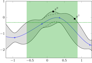
$y_{t}^{\bullet}$ is represented by the horizontal dotted green line on Figure 2. $\mathfrak{R}_{t}$ is defined as :

$$\mathfrak{R}_{t}=\Big{\{}x\in\mathcal{X}\mid\widehat{f}_{t}^{+}(x)\geq y_{t}^{\bullet}\Big{\}}~{}.$$

$\mathfrak{R}_{t}$ discard the locations where $x^{\star}$ does not belong with high probability. It is represented in green on Figure 2. We refer to [24] for related work in the special case of deterministic Gaussian Process Bandits.

In the sequel, we will use a modified version of the relevant region which also contains $\operatorname*{\arg\!\max}_{x\in\mathcal{X}}\widehat{f}_{t+1}^{+}(x)$ with high probability. The novel relevant region is formally defined by :

$$\mathfrak{R}_{t}^{+}=\Big{\{}x\in\mathcal{X}\mid\widehat{\mu}_{t}(x)+2\sqrt{\beta_{t+1}}\widehat{\sigma}_{t}(x)\geq y_{t}^{\bullet}\Big{\}}~{}.$$ (6)

Using $\mathfrak{R}_{t}^{+}$ instead of $\mathfrak{R}_{t}$ guarantees that the queries at iteration $t$ will leave an impact on the future choices at iteration $t+1$.

3.3 GP-UCB-PE

for $t=0,\dots,T$ do

       Compute $\widehat{\mu}_{t}$ and $\widehat{\sigma}_{t}$ with Eq.1 and Eq.2

       $x_{t}^{0}\leftarrow\operatorname*{\arg\!\max}_{x\in\mathcal{X}}\widehat{f}_{t}^{+}(x)$

       Compute $\mathfrak{R}_{t}^{+}$ with Eq.6

       for $k=1,\dots,K-1$ do

             Compute $\widehat{\sigma}_{t}^{(k)}$ with Eq.2

             $x_{t}^{k}\leftarrow\operatorname*{\arg\!\max}_{x\in\mathfrak{R}_{t}^{+}}\widehat{\sigma}_{t}^{(k)}(x)$

            

      Query $\{x_{t}^{k}\}_{k<K}$

      

Algorithm 1 GP-UCB-PE

We present here the Gaussian Process Upper Confidence Bound with Pure Exploration algorithm, GP-UCB-PE, a novel algorithm combining two strategies to determine the queries $\{x_{t}^{k}\}_{k<K}$ for batches of size $K$. The first location is chosen according to the GP-UCB rule,

$$x_{t}^{0}=\operatorname*{\arg\!\max}_{x\in\mathcal{X}}\widehat{f}_{t}^{+}(x)~{}.$$ (7)

This single rule is enough to tackle the exploration/exploitation tradeoff. The value of $\beta_{t}$ balances between exploring uncertain regions (high posterior variance $\widehat{\sigma}_{t}^{2}(x)$) and focusing on the supposed location of the maximum (high posterior mean $\widehat{\mu}_{t}(x)$). This policy is illustrated with the point $x^{0}$ on Figure 2.

The $K-1$ remaining locations are selected via Pure Exploration restricted to the region $\mathfrak{R}_{t}^{+}$. We aim to maximize $I_{t}(\mathbf{X}_{t}^{K-1})$, the information gain about $f$ by the locations $\mathbf{X}_{t}^{K-1}=\{x_{t}^{k}\}_{1\leq k<K}$ [25]. Formally, $I_{t}(\mathbf{X})$ is the reduction of entropy when knowing the values of the observations $\mathbf{Y}$ at $\mathbf{X}$, conditioned on $\mathbf{X}_{t}$ the observations we have seen so far,

$$I_{t}(\mathbf{X})=H(\mathbf{Y})-H(\mathbf{Y}\mid\mathbf{X}_{t})~{}.$$ (8)

Finding the $K-1$ points that maximize $I_{t}$ for any integer $K$ is known to be -complete [26]. However, due to the submodularity of $I_{t}$ [4], it can be efficiently approximated by the greedy procedure which selects the points one by one and never backtracks. For a Gaussian distribution, $H(\mathcal{N}(\mathbf{\mu},\mathbf{C}))=\frac{1}{2}\log\det(2\pi e\mathbf{C})$. We thus have $I_{t}(\mathbf{X})\in\mathcal{O}(\log\det\mathbf{\Sigma})$, where $\mathbf{\Sigma}$ is the covariance matrix of $\mathbf{X}$. For GP, the location of the single point that maximizes the information gain is easily computed by maximizing the posterior variance. For all $~{}1\leq k<K$ our greedy strategy selects the following points one by one,

$$x_{t}^{k}=\operatorname*{\arg\!\max}_{x\in\mathfrak{R}_{t}^{+}}\widehat{\sigma}_{t}^{(k)}(x)~{},$$ (9)

where $\widehat{\sigma}_{t}^{(k)}$ is the updated variance after choosing $\{x_{t}^{k^{\prime}}\}_{k^{\prime}<k}$. We use here the fact that the posterior variance does not depend on the values $y_{t}^{k}$ of the observations, but only on their position $x_{t}^{k}$. One such point is illustrated with $x^{1}$ on Figure 2. These $K-1$ locations reduce the uncertainty about $f$, improving the guesses of the UCB procedure by $x_{t}^{0}$. The overall procedure is shown in Algorithm 1.

Figure 2: Two queries of GP-UCB-PE on the previous example. The lower confidence bound on the maximum is represented by the horizontal dotted green line at $y_{t}^{\bullet}$. The relevant region $\mathfrak{R}$ is shown in light green (without edges). The first query $x^{0}$ is the maximizer of $\widehat{f}^{+}$. We show in dashed line the upper and lower bounds with the update of $\widehat{\sigma}$ after having selected $x^{0}$. The second query $x^{1}$ is the one maximizing the uncertainty inside $\mathfrak{R}^{+}$, an extension of $\mathfrak{R}$ which is not illustrated here.

3.4 Numerical Complexity

Even if the numerical cost of GP-UCB-PE is insignificant in practice compared to the cost of the evaluation of $f$, the complexity of the exact computations of the variances (Eq.2) is in $\mathcal{O}(n^{3})$ and might by prohibitive for large $n=tK$. One can reduce drastically the computation time by means of Lazy Variance Calculation [19], built on the fact that $\widehat{\sigma}_{t}(x)$ always decreases when $t$ increases for all $x\in\mathcal{X}$. We further mention that efficient approximated inference algorithms such as the EP approximation and MCMC sampling [27] can be used in order to face the challenge of large $n$.

4 Regret Bounds

4.1 Main Result

The main theoretical result of this article is the upper bound on the regret formulated in Theorem 4.1. We need to adjust the parameter $\beta_{t}$ such that $f(x)$ is contained by the high confidence region for all iterations $t$ with probability at least $1-\delta$ for a fixed $0<\delta<1$.

• If $\mathcal{X}$ is finite, then we choose $\beta_{t}=2\log(\left\lvert\mathcal{X}\right\rvert\frac{\pi_{t}}{\delta})$ where $\pi_{t}>0$ such that $\sum_{t=0}^{\infty}\pi_{t}^{-1}=1$. We set for example $\beta_{t}=2\log\big{(}\left\lvert\mathcal{X}\right\rvert t^{2}\frac{\pi^{2}}{6\delta}\big{)}$.

• If $\mathcal{X}\subset[0,r]^{d}$ is compact and convex, we need the following bounds on the derivatives of $f$,

  $$\exists a,b>0,\ \forall j\leq d,\ \ \Pr\left(\sup_{x\in\mathcal{X}}\left\lvert\frac{\partial f}{\partial x_{j}}\right\rvert>L\right)\leq ae^{-\frac{L^{2}}{b^{2}}}~{}.$$

  Then, we can set the parameter $\beta_{t}$ to :

  $$\beta_{t}=2\log\left(t^{2}\frac{2\pi^{2}}{3\delta}\right)+2d\log\left(t^{2}dbr\sqrt{\log\Big{(}\frac{4da}{\delta}\Big{)}}\right)~{}.$$

The regret bound are expressed in term of $\gamma_{TK}$, the maximum information gain (Eq. 8) obtainable by a sequence of $TK$ queries,

$$\gamma_{t}=\max_{\mathbf{X}\subset\mathcal{X},\left\lvert\mathbf{X}\right\rvert=t}I_{0}(\mathbf{X})~{}.$$

Under these assumptions, we obtain the following result.

Theorem 4.1

Fix $0<\delta<1$ and consider the calibration of $\beta_{t}$ defined as above, assuming $f\sim GP(0,k)$ with bounded variance, $\forall x\in\mathcal{X},~{}k(x,x)\leq 1$, then the batch cumulative regret incurred by GP-UCB-PE on $f$ is bounded by $\mathcal{O}\Big{(}\sqrt{\frac{T}{K}\beta_{T}\gamma_{TK}}\Big{)}$ whp, More precisely, with $C_{1}=\frac{4}{\log(1+\sigma^{-2})}$, and $C_{2}=\frac{\pi}{\sqrt{6}}$, $\forall T,$

$$\Pr\left(R_{T}^{K}\leq\sqrt{C_{1}\frac{T}{K}\beta_{T}\gamma_{TK}+C_{2}}\right)\geq 1-\delta~{}.$$

For the full cumulative regret $R_{TK}$ we obtain similar bounds with $C_{1}=\frac{36}{\log(1+\sigma^{-2})}$

$$\Pr\left(R_{TK}\leq\sqrt{C_{1}TK\beta_{T}\gamma_{TK}+C_{2}}\right)\geq 1-\delta~{}.$$

4.2 Discussion

When $K\ll T$, the upper bound for $R_{T}^{K}$ is better than the one of sequential GP-UCB by an order of $\sqrt{K}$, and equivalent for $R_{TK}$, when the regrets for all the points in the batch matter. Compared to [19], we remove the need of the initialization phase. GP-UCB-PE does not need either to multiply the uncertainty parameter $\beta_{t}$ by $\exp(\gamma_{TK}^{\text{init}})$ where $\gamma_{TK}^{\text{init}}$ is equal to the maximum information gain obtainable by a sequence of $TK$ queries after the initialization phase. The improvement can be doubly exponential in the dimension $d$ in the case of RBF Kernels. To the best of our knowledge, no regret bounds have been proven for the Simulation Matching algorithm.

The values of $\gamma_{TK}$ for different common kernel are reported in Table 1, where $d$ is the dimension of the space considered and $\alpha=\frac{d(d+1)}{2\nu+d(d+1)}\leq 1$, $\nu$ being the Matérn parameter. We also compare on Table 1 the general forms of the bounds for the regret obtained by GP-UCB-PE and GP-BUCB up to constant terms. The cumulative regret we obtained with RBF Kernel is of the form $\tilde{\mathcal{O}}\Big{(}\sqrt{\frac{T}{K}(\log TK)^{d}}\Big{)}$ against $\tilde{\mathcal{O}}\Big{(}\exp((\frac{2d}{e})^{d})\sqrt{\frac{T}{K}(\log TK)^{d}}\Big{)}$ for GP-BUCB.

4.3 Proofs of the Main Result

In this section, we analyze theoretically the regret bounds for the GP-UCB-PE algorithm. We provide here the main steps for the proof of Theorem 4.1. On one side the UCB rule of the algorithm provides a regret bounded by the information we have on $f$ conditioned on the values observed so far. On the other side, the Pure Exploration part gathers information and therefore accelerates the decrease in uncertainty. We refer to [19] for the proofs of the bounds for GP-BUCB.

For the sake of concision, we introduce the notations $\sigma_{t}^{k}$ for $\widehat{\sigma}_{t}^{(k)}(x_{t}^{k})$ and $\sigma_{t}^{0}$ for $\widehat{\sigma}_{t}(x_{t}^{0})$. We simply bound $r_{t}^{K}$ the regret for the batch at iteration $t$ by the simple regret $r_{t}^{(0)}$ for the single query chosen via the UCB rule. We then give a bound for $r_{t}^{(0)}$ which is proportional to the posterior deviations $\sigma_{t}^{0}$. Knowing that the sum of all $(\sigma_{t}^{k})^{2}$ is not greater than $C_{1}\gamma_{TK}$, we want to prove that the sum of the $(\sigma_{t}^{0})^{2}$ is less than this bound divided by $K$. The arguments are based on the fact that the posterior for $f(x)$ is Gaussian, allowing us to choose $\beta_{t}$ such that :

$$\forall x\in\mathcal{X},\forall t<T,\ f(x)\in[\widehat{f}_{t}^{-}(x),\widehat{f}_{t}^{+}(x)]$$

holds with high probability. Here and in the following, “with high probability” or whp means “with probability at least $1-\delta$” for any $0<\delta<1$, the definition of $\beta_{t}$ being dependent of $\delta$.

Table 1: General Forms of Regret Bounds for GP-UCB-PE and GP-BUCB

	GP-UCB-PE		GP-BUCB
$R_{T}^{K}$	$\sqrt{\frac{T\log T}{K}\gamma_{TK}}$		$C\sqrt{\frac{T\log TK}{K}\gamma_{TK}}$
Kernel	Linear	RBF		Matérn
$\gamma_{TK}$	$d\log{TK}$	$(\log TK)^{d+1}$		$(TK)^{\alpha}\log TK$
$C$	$\exp(\frac{2}{e})$	$\exp((\frac{2d}{e})^{d})$		$e$

Lemma 1

For finite $\mathcal{X}$, we have $r_{t}^{K}\leq r_{t}^{(0)}\leq 2\sqrt{\beta_{t}}\sigma_{t}^{0}$, and for compact and convex $\mathcal{X}$ following the assumptions of Theorem 4.1, $r_{t}^{K}\leq r_{t}^{(0)}\leq 2\sqrt{\beta_{t}}\sigma_{t}^{0}+\frac{1}{t^{2}}$, holds with probability at least $1-\delta$.

We refer to [6] (Lemmas 5.2, 5.8) for the detailed proof of the bound for $r_{t}^{(0)}$.

Now we show an intermediate result bounding the deviations at the points $x_{t+1}^{0}$ by the one at the points $x_{t}^{K-1}$.

Lemma 2

The deviation of the point selected by the UCB policy is bounded by the one for the last point selected by the PE policy at the previous iteration, whp, $\forall t<T,\ \sigma_{t+1}^{0}\leq\sigma_{t}^{K-1}$

Proof

By the definitions of $x_{t+1}^{0}$ (Eq.7), we have $\widehat{f}_{t+1}^{+}(x_{t+1}^{0})\geq\widehat{f}_{t+1}^{+}(x_{t}^{\bullet})$. Then, we know with high probability that $\forall x\in\mathcal{X},\forall t<T,\ \widehat{f}_{t+1}^{+}(x)\geq\widehat{f}_{t}^{-}(x)$. We can therefore claim whp $\widehat{f}_{t+1}^{+}(x_{t+1}^{0})\geq y_{t}^{\bullet}$, and thus that $x_{t+1}^{0}\in\mathfrak{R}_{t}^{+}$ whp.

We have as a result by the definition of $x_{t}^{k-1}$ (Eq.9) that $\widehat{\sigma}_{t}^{(k-1)}(x_{t+1}^{0})\leq\widehat{\sigma}_{t}^{(k-1)}(x_{t}^{k-1})$ whp. Using the “Information never hurts” principle [28], we know that the entropy of $f(x)$ for all location $x$ decreases while we observe points $x_{t}$. For GP, the entropy is also a non-decreasing function of the variance, so that :

$$\forall x\in\mathcal{X},\ \widehat{\sigma}_{t+1}^{(0)}(x)\leq\widehat{\sigma}_{t}^{(k-1)}(x)~{}.$$

We thus prove ${\sigma_{t+1}^{0}\leq\sigma_{t}^{k-1}}$.

Lemma 3

The sum of the deviations of the points selected by the UCB policy are bounded by the one for all the selected points divided by $K$, whp,

$$\sum_{t=0}^{T-1}\sigma_{t}^{0}\leq\frac{1}{K}\sum_{t=0}^{T-1}\sum_{k=0}^{K-1}\sigma_{t}^{k}~{}.$$

Proof

Using Lemma 2 and the definitions of the $x_{t}^{k}$, we have that $\sigma_{t+1}^{0}\leq\sigma_{t}^{k}$ for all $k\geq 1$. Summing over $k$, we get for all $t\geq 0$, $\sigma_{t}^{0}+(K-1)\sigma_{t+1}^{0}\leq\sum_{k=0}^{K-1}\sigma_{t}^{k}$. Now, summing over $t$ and with $\sigma_{0}^{0}\geq 0$ and $\sigma_{T}^{0}\geq 0$, we obtain the desired result.

Next, we can bound the sum of all posterior variances $(\sigma_{t}^{k})^{2}$ via the maximum information gain for a sequence of $TK$ locations.

Lemma 4

The sum of the variances of the selected points are bounded by a constant factor times $\gamma_{TK}$, $\exists C_{1}^{\prime}\in\mathbb{R},~{}\sum_{t<T}\sum_{k<K}(\sigma_{t}^{k})^{2}\leq C_{1}^{\prime}\gamma_{TK}$ where $\gamma_{TK}$ is the maximum information gain obtainable by a sequential procedure of length $TK$.

Proof

We know that the information gain for a sequence of $T$ locations $x_{t}$ can be expressed in terms of the posterior variances $(\widehat{\sigma}_{t-1}(x_{t}))^{2}$. The deviations $\sigma_{t}^{k}$ being independent of the observations $y_{t}^{k}$, the same equality holds for the posterior variances $(\widehat{\sigma}^{(k)}_{t}(x_{t}^{k}))^{2}$. See Lemmas 5.3 and 5.4 in [6] for the detailed proof, giving $C_{1}^{\prime}=\frac{2}{\log(1+\sigma^{-2})}$.

Lemma 5

The cumulative regret can be bound in terms of the maximum information gain, whp, $\exists C_{1},C_{2}\in\mathbb{R}$,

$$\sum_{t<T}r_{t}^{K}\leq\sqrt{\frac{T}{K}C_{1}\beta_{T}\gamma_{TK}+C_{2}}~{}.$$

Proof

Using the previous lemmas and the fact that $\beta_{t}\leq\beta_{T}$ for all $t\leq T$, we have in the case of finite $\mathcal{X}$, whp,

$$\sum_{t<T}r_{t}^{K} \leq\sum_{t<T}2\sqrt{\beta_{t}}\sigma_{t}^{0}\text{~{}, by Lemma \ref{lem:reg}}$$

$$\leq 2\sqrt{\beta_{T}}\frac{1}{K}\sum_{t<T}\sum_{k<K}\sigma_{t}^{k}\text{~{}, by Lemma \ref{lem:dev_ucb}}$$

$$\leq 2\sqrt{\beta_{T}}\frac{1}{K}\sqrt{TK\sum_{t<T}\sum_{k<K}(\sigma_{t}^{k})^{2}}\text{~{}, by Cauchy-Schwarz}$$

$$\leq 2\sqrt{\beta_{T}}\frac{1}{K}\sqrt{TKC^{\prime}_{1}\gamma_{TK}}\text{~{}, by Lemma \ref{lem:gamma_tk}}$$

$$\leq\sqrt{\frac{T}{K}C_{1}\beta_{T}\gamma_{TK}}\text{ with }C_{1}=\frac{4}{\log(1+\sigma^{-2})}~{}.$$

For compact and convex $\mathcal{X}$, a similar reasoning gives :

$$R_{T}^{K}\leq\sqrt{\frac{T}{K}C_{1}\beta_{T}\gamma_{TK}+C_{2}}\text{ with }C_{2}=\frac{\pi}{\sqrt{6}}<2~{}.$$

Lemma 5 conclude the proof of Theorem 4.1 for the regret $R_{T}^{K}$. The analysis for $R_{TK}$ is simpler, using the Lemma 6 which bounds the regret for the Pure Exploration queries, leading to $C_{1}=\frac{36}{\log(1+\sigma^{-2})}$.

Lemma 6

The regret for the queries $x_{t}^{k}$ selected by Pure Exploration in $\mathfrak{R}_{t}^{+}$ are bounded whp by, $6\sqrt{\beta_{t}}\widehat{\sigma}_{t}(x_{t}^{k})$.

Proof

As in Lemma 1, we have whp, for all $t\leq T$ and $k\geq 1$,

$$r_{t}^{(k)} \leq\widehat{\mu}_{t}(x^{\star})+\sqrt{\beta_{t}}\widehat{\sigma}_{t}(x^{\star})-\widehat{\mu}_{t}(x_{t}^{k})+\sqrt{\beta_{t}}\widehat{\sigma}_{t}(x_{t}^{k})$$

$$\leq\widehat{f}_{t}^{-}(x^{\bullet}_{t})+2\sqrt{\beta_{t}}\widehat{\sigma_{t}}(x^{\star})-\widehat{\mu}_{t}(x_{t}^{k})+\sqrt{\beta_{t}}\widehat{\sigma}_{t}(x_{t}^{k})\text{ by definition of }x^{\bullet}_{t}$$

$$\leq\widehat{\mu}_{t}(x_{t}^{k})+2\sqrt{\beta_{t+1}}\widehat{\sigma}_{t}(x_{t}^{k})+2\sqrt{\beta_{t}}\widehat{\sigma}_{t}(x_{t}^{k})-\widehat{\mu}_{t}(x_{t}^{k})+\sqrt{\beta_{t}}\widehat{\sigma}_{t}(x_{t}^{k})\text{ by definition of }\mathfrak{R}_{t}^{+}$$

$$\leq 3\sqrt{\beta_{t}}\widehat{\sigma}_{t}(x_{t}^{k})+2\sqrt{\beta_{t}}\widehat{\sigma}_{t}(x_{t}^{k})+\sqrt{\beta_{t}}\widehat{\sigma}_{t}(x_{t}^{k})\text{ by definition of }\beta_{t+1}$$

$$\leq 6\sqrt{\beta_{t}}\widehat{\sigma}_{t}(x_{t}^{k})~{}.$$

To conclude the analysis of $R_{TK}$ and prove Theorem 4.1, it suffices to use then the last four steps of Lemma 5.

5 Experiments

(a) Himmelblau

(b) Gaussian mixture

Figure 3: Visualization of the synthetic functions used for assessment

5.1 Protocol

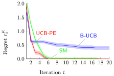
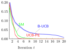
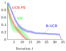
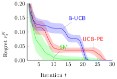
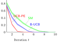
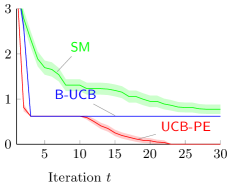
We compare the empirical performances of our algorithm against the state of the art of global optimization by batches, GP-BUCB [19] and SM-UCB [20]. The tasks used for assessment come from three real applications and two synthetic problems described here. The results are shown in Figure 4. For all datasets and algorithms, the size of the batches $K$ was set to $10$ and the learners were initialized with a random subset of $20$ observations $(x_{i},y_{i})$. The curves on Figure 4 show the evolution of the regret $R_{t}^{K}$ in term of iteration $t$. We report the average value with the confidence interval over $64$ experiments. The parameters for the prior distribution, like the bandwidth of the RBF Kernel, were chosen by maximization of the marginal likelihood.

5.2 Description of Data Sets

Generated GP.

The Generated GP functions are random GPs drawn from a Matérn kernel (Eq. 3) in dimension $2$, with the kernel bandwidth set to $\frac{1}{4}$, the Matérn parameter $\nu=3$ and noise variance $\sigma^{2}$ set to $1$.

Gaussian Mixture.

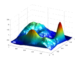
This synthetic function comes from the addition of three $2$-D Gaussian functions. at $(0.2,0.5)$, $(0.9,0.9)$, and the maximum at $(0.6,0.1)$. We then perturb these Gaussian functions with smooth variations generated from a Gaussian Process with Matérn Kernel and very few noise. It is shown on Figure 3(b). The highest peak being thin, the sequential search for the maximum of this function is quite challenging.

Himmelblau Function.

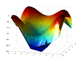
The Himmelblau task is another synthetic function in dimension $2$. We compute a slightly tilted version of the Himmelblau’s function, and take the opposite to match the challenge of finding its maximum. This function presents four peaks but only one global maximum. It gives a practical way to test the ability of a strategy to manage exploration/exploitation tradeoffs. It is represented in Figure 3(a).

Mackey-Glass Function.

The Mackey-Glass delay-differential equation is a chaotic system in dimension $6$, but without noise. It models real feedback systems and is used in physiological domains such as hematology, cardiology, neurology, and psychiatry. The highly chaotic behavior of this function makes it an exceptionally difficult optimization problem. It has been used as a benchmark for example by [29].

Tsunamis.

Recent post-tsunami survey data as well as the numerical simulations of [30] have shown that in some cases the run-up, which is the maximum vertical extent of wave climbing on a beach, in areas which were supposed to be protected by small islands in the vicinity of coast, was significantly higher than in neighboring locations. Motivated by these observations [31] investigated this phenomenon by employing numerical simulations using the VOLNA code [32] with the simplified geometry of a conical island sitting on a flat surface in front of a sloping beach. Their setup was controlled by five physical parameters and their aim was to find with confidence and with the least number of simulations the maximum run-up amplification on the beach directly behind the island, compared with the run-up on a lateral location, not influenced by the presence of the island. Since this problem is too complex to treat analytically, the authors had to solve numerically the Nonlinear Shallow Water Equations.

(a) Generated GP

(b) Himmelblau

(c) Gaussian Mixture

(d) Mackey-Glass

(e) Tsunamis

(f) Abalone

Figure 4: Experiments on several real and synthetics tasks. The curves show the decay of the mean of the simple regret $r_{t}^{K}$ with respect to the iteration $t$, over $64$ experiments. We show with the translucent area the confidence intervals.

Abalone.

The challenge of the Abalone dataset is to predict the age of a specie of sea snails from physical measurements. It comes from the study by [33] and it is provided by the UCI Machine Learning Repository. We use it as a maximization problem in dimension $8$.

5.3 Comparison of Algorithms

The algorithm SM —Simulation Matching— described in [20], with UCB base policy, has shown similar results to GP-UCB-PE on synthetic functions (Figures 4(a), 4(b), 4(c)) and even better results on chaotic problem without noise (Figure 4(d)), but performs worse on real noisy data (Figures 4(e), 4(f)). On the contrary, the initialization phase of GP-BUCB leads to good regret on difficult real tasks (Figure 4(e)), but looses time on synthetic Gaussian or polynomial ones (Figures 4(a), 4(b), 4(c)). The number of dimensions of the Abalone task is already a limitation for GP-BUCB with the RBF kernel, making the initialization phase time-consuming. The mean regret for GP-BUCB converges to zero abruptly after the initialization phase at iteration $55$, and is therefore not visible on Figure 4(f), as for 4(c) where its regret decays at iteration $34$.

GP-UCB-PE achieves good performances on both sides. We obtained better regret on synthetic data as well as on real problems from the domains of physics and biology. Moreover, the computation time of SM was two order of magnitude longer than the others.

6 Conclusion

We have presented the GP-UCB-PE algorithm which addresses the problem of finding in few iterations the maximum of an unknown arbitrary function observed via batches of $K$ noisy evaluations. We have provided theoretical bounds for the cumulative regret obtained by GP-UCB-PE in the Gaussian Process settings. Through parallelization, these bounds improve the ones for the state-of-the-art of sequential GP optimization by a ratio of $\sqrt{K}$, and are strictly better than the ones for GP-BUCB, a concurrent algorithm for parallel GP optimization. We have compared experimentally our method to GP-BUCB and SM-UCB, another approach for parallel GP optimization lacking of theoretical guarantees. These empirical results have confirmed the effectiveness of GP-UCB-PE on several applications.

The strategy of combining in the same batch some queries selected via Pure Exploration is an intuitive idea that can be applied in many other methods. We expect for example to obtain similar results with the Maximum Expected Improvement policy (MEI). Any proof of regret bound that relies on the fact that the uncertainty decreases with the exploration should be easily adapted to a paralleled extension with Pure Exploration.

On the other hand, we have observed in practice that the strategies which focus more on exploitation often lead to faster decrease of the regret, for example the strategy that uses $K$ times the GP-UCB criterion with updated variance. We conjecture that the regret for this strategy is unbounded for general GPs, justifying the need for the initialization phase of GP-BUCB. However, it would be relevant to specify formally the assumptions needed by this greedy strategy to guarantee good performances.

References

- [1] Hennig, P., Schuler, C.J.: Entropy search for information-efficient global optimization. Journal of Machine Learning Research 13 (2012) 1809–1837
- [2] Fedorov, V.V.: Theory of Optimal Experiments. Academic Press (1972)
- [3] Chen, B., Castro, R., Krause, A.: Joint optimization and variable selection of high-dimensional gaussian processes. In: Proceedings of ICML, ACM (2012)
- [4] Guestrin, C., Krause, A., Singh, A.: Near-optimal sensor placements in Gaussian processes. In: Proceedings of ICML, ACM (2005) 265–272
- [5] Grünewälder, S., Audibert, J.Y., Opper, M., Shawe-Taylor, J.: Regret Bounds for Gaussian Process Bandit Problems. In: Proceedings of AISTATS, MIT Press (2010) 273–280
- [6] Srinivas, N., Krause, A., Kakade, S.M., Seeger, M.W.: Information-theoretic regret bounds for gaussian process optimization in the bandit setting. IEEE Transactions on Information Theory 58(5) (2012) 3250–3265
- [7] Mockus, J.: Bayesian approach to global optimization: theory and applications. Mathematics and its applications (Kluwer Academic Publishers).: Soviet series. Kluwer Academic (1989)
- [8] Mes, M.R., Powell, W.B., Frazier, P.I.: Hierarchical knowledge gradient for sequential sampling. Journal of Machine Learning Research 12 (2011) 2931–2974
- [9] Carpentier, A., Lazaric, A., Ghavamzadeh, M., Munos, R., Auer, P.: Upper-confidence-bound algorithms for active learning in multi-armed bandits. In: Proceedings of the ALT, Springer-Verlag (2011) 189–203
- [10] Chen, Y., Krause, A.: Near-optimal batch mode active learning and adaptive submodular optimization. In: Proceedings of ICML, ACM (2013)
- [11] Auer, P., Cesa-Bianchi, N., Fischer, P.: Finite-time analysis of the multiarmed bandit problem. Machine Learning 47(2-3) (2002) 235–256
- [12] Auer, P., Ortner, R., Szepesvári, C.: Improved rates for the stochastic continuum-armed bandit problem. In: Proceedings of COLT, Omnipress (2007) 454–468
- [13] Coquelin, P.A., Munos, R.: Bandit algorithms for tree search. In: Proceedings of UAI, AUAI Press (2007) 67–74
- [14] Kleinberg, R.: Nearly tight bounds for the continuum-armed bandit problem. In: Advances in NIPS, MIT Press (2004) 697–704
- [15] Kocsis, L., Szepesvári, C.: Bandit based monte-carlo planning. In: Proceedings of ECML, Springer (2006) 282–293
- [16] Audibert, J.Y., Bubeck, S., Munos, R.: Bandit view on noisy optimization. In: Optimization for Machine Learning. MIT Press (2011) 431–454
- [17] Sutton, R.S., Barto, A.G.: Reinforcement Learning: An Introduction. A Bradford Book (1998)
- [18] Bubeck, S., Munos, Stoltz, G., Szepesvári, C.: Online optimization in x-armed bandits. In: Advances in NIPS, Curran Associates, Inc. (2008) 201–208
- [19] Desautels, T., Krause, A., Burdick, J.: Parallelizing exploration-exploitation tradeoffs with gaussian process bandit optimization. In: Proceedings of ICML, icml.cc / Omnipress (2012)
- [20] Azimi, J., Fern, A., Fern, X.: Batch bayesian optimization via simulation matching. In: Advances in NIPS, Curran Associates, Inc. (2010) 109–117
- [21] Bubeck, S., Cesa-Bianchi, N.: Regret analysis of stochastic and nonstochastic multi-armed bandit problems. Foundations and Trends in Machine Learning 5(1) (2012) 1–122
- [22] Bubeck, S., Munos, R., Stoltz, G.: Pure exploration in multi-armed bandits problems. In: Proceedings of ALT. Springer-Verlag (2009) 23–37
- [23] Rasmussen, C.E., Williams, C.: Gaussian Processes for Machine Learning. MIT Press (2005)
- [24] de Freitas, N., Smola, A.J., Zoghi, M.: Exponential regret bounds for gaussian process bandits with deterministic observations. In: Proceedings of ICML, icml.cc / Omnipress (2012)
- [25] Cover, T.M., Thomas, J.A.: Elements of Information Theory. Wiley-Interscience (1991)
- [26] Ko, C., Lee, J., Queyranne, M.: An exact algorithm for maximum entropy sampling. Operations Research (1995) 684–691
- [27] Kuss, M., Pfingsten, T., Csató, L., Rasmussen, C.E., Kuss, M., Pfingsten, T., Csató, L., Rasmussen, C.E.: Approximate inference for robust gaussian process regression (2005)
- [28] Krause, A., Guestrin, C.: Near-optimal nonmyopic value of information in graphical models. In: Proceedings of UAI, AUAI Press (2005) 324–331
- [29] Flake, G.W., Lawrence, S.: Efficient svm regression training with smo. Machine Learning 46(1-3) (2002) 271–290
- [30] Hill, E.M., Borrero, J.C., Huang, Z., Qiu, Q., Banerjee, P., Natawidjaja, D.H., Elosegui, P., Fritz, H.M., Suwargadi, B.W., Pranantyo, I.R., Li, L., Macpherson, K.A., Skanavis, V., Synolakis, C.E., Sieh, K.: The 2010 mw 7.8 mentawai earthquake: Very shallow source of a rare tsunami earthquake determined from tsunami field survey and near-field gps data. J. Geophys. Res. 117 (2012) B06402–
- [31] Stefanakis, T.S., Dias, F., Vayatis, N., Guillas, S.: Long-wave runup on a plane beach behind a conical island. In: Proceedings of WCEE. (2012)
- [32] Dutykh, D., Poncet, R., Dias, F.: The VOLNA code for the numerical modelling of tsunami waves: generation, propagation and inundation. European Journal of Mechanics B/Fluids 30 (2011) 598–615
- [33] Nash, W., Tasmania. Marine Research Laboratories: The population biology of abalone (haliotis species) in tasmania: Blacklip abalone (h. rubra) from the north coast and the islands of bass strait. Technical report, Tasmania. Sea Fisheries Division (1994)