Oscillation of high energy neutrinos in Choked GRBs

Abstract

It is believed that choked gamma-ray bursts (CGRBs) are the potential candidates for the production of high energy neutrinos in GeV-TeV energy range. These CGRBs out number the successful GRBs by many orders. So it is important to observe neutrinos from these cosmological objects with the presently operating neutrino telescope IceCube. We study the three flavor neutrino oscillation of these high energy neutrinos in the presupernova star environment which is responsible for the CGRB. For the presupernova star we consider three different models and calculate the neutrino oscillation probabilities, as well as neutrino flux on the surface of these star. The matter effect modifies the neutrino flux of different flavors on the surface of the star. We have also calculated the flux of these high energy neutrinos on the surface of the Earth. We found that for neutrino energies below $\leq 10$ TeV the flux ratio does not amount to 1:1:1, whereas for higher energy neutrinos it does.

I Introduction

The long Type ($\geq 2$ s) of gamma-ray bursts (GRBs) constitute about 3/4 of the total observed GRBs. The observed correlations of the following GRBs with supernovae (SNe), GRB980425/SN 1998bw Galama:1998ea ,GRB 030329/SN 2003dh Mazzali:2003np , GRB 031203/SN 2003lwThomsen:2004sp and GRB 021211/SN 2002ltDellaValle:2003uj show that core collapse of massive stars are related to long type of GRBs. These mostly occur in star forming regionsWoosley:2006fn ; Zhang:2009uf . The core collapse of massive stars resulting in a relativistic jet which breaks through the stellar envelope is a widely discussed scenario for gamma-ray burst production. In this scenario, the gamma-rays are produced by synchrotron and/or inverse-Compton scattering of Fermi accelerated electrons in optically thin shock, when the jet has emerged out of the stellar envelope. These same shocks are also responsible for the acceleration of the protons into relativistic velocities and collisions of these with the MeV photons produce neutrinos of energy $\sim 100$ TeVWaxman:1997ti .

The formation of jets may be a common phenomena in a collapsar scenario and depending on the composition (baryon load) all the jets may not have sufficient energy and momentum to punch trough the stellar envelope. From the observed rate of GRBs, only about $\leq 10^{-3}$ core collapse supernovae produce highly relativistic jets (Lorentz factor $\Gamma\geq 100$) which can penetrate through the envelope and produce GRB events in an optically thin environment outside the starBerger:2003kg . On the other hand, a large fraction of them will fail to emerge out of the envelope, which may give rise to orphan radio afterglow instead of $\gamma$-ray emission. However when the jets are making their way through the star they can accelerate protons to energy $\geq 10^{5}\,{\rm GeV}$ through internal shocks well inside the stellar envelope. Also the buried jet produces thermal X-ray at $\sim 1\,{\rm keV}$ which acts as the target for the delta-resonance to produce $\geq$ 5 TeV energy neutrinos through photopion production, which penetrates through the envelopeMeszaros:2001ms . There can also be neutrino production due to $pp$ and $pn$ collisions involving relativistic protons from the buried jet and the thermal nucleons from the jet and the surroundingRazzaque:2004yv . However, when the jets are still making their way through the star, precursor TeV neutrinos are inherent to the collapse of a massive star irrespective of whether GRB is produced or not. Forward moving jets which are unable to emerge out of the envelope may be rich in baryons which make them mildly relativistic, but at the same time efficient producers of TeV neutrinos through photomeson interaction. The detection of low luminosity GRB 060218Campana:2006qe suggests that their number (low luminosity GRBs and dark GRBs) may be quite large compared to the high luminosity GRBs, which can probably contribute more to the TeV neutrino backgroundLiang:2007 than the high luminosity ones and could be detectable by present day neutrino telescopes (e.g. in IceCube) which can shed more light on the nature of the central engine, as well as the acceleration mechanism of high energy cosmic rays in the presupernova starRazzaque:2003uv ; Razzaque:2005bh . From an individual collapse/GRB burst at a distance $z\sim 1$, about 0.1-10 upward going muon events can be detected in a ${\rm km}^{3}$ detectorMeszaros:2001ms .

These high energy neutrinos propagating through the presupernova star with a heavy envelop can oscillate to other flavors due to the matter effect. In fact the mater effect is well known for neutrinos propagating in the sun, supernova as well as in the early Universe. In optically thick hidden sources where gamma-rays are not observed directly and $\sim{\rm TeV}$ neutrinos are produced due to $p\gamma$, $pp$ and $pn$ collision, the flux ratio at the production site and on the surface of the star may be different due to matter effect on their oscillation. Recently for two neutrino flavors it is shown that for the choked GRBs, the multi-TeV neutrino signals proposed by Mészáros and Waxman Meszaros:2001ms can undergo substantial resonance oscillation before escaping from the He envelope if the neutrino oscillation parameters are in the atmospheric neutrino oscillation range. This would alter the neutrino flavor ratio escaping from the stellar envelope, and subsequently the detected flavor ratio on EarthSahu:2010ap . So in this context it is important to study the matter effect of the presupernova star on the oscillation of high energy neutrinos emerging out of it.

The neutrino oscillation in vacuum and matter has been discussed extensively for solar, atmospheric as well as accelerator and reactor experiments. Models of three flavor neutrino oscillations in constant matter densityBarger:1980tf ; Kim:1986vg ; Zaglauer:1988gz , linearly varying densityPetcov:1987xd ; Lehmann:2000ey and exponentially varying densityOsland:1999et have been studied. In Ref.Ohlsson:1999xb T. Ohlsson and H. Snellman have developed an analytic formalism for the oscillation of three flavor neutrinos in the matter background with varying density, where they use the plane wave approximation for the neutrinos (henceforth we refer to this as OS formalism). Here the evolution operator and the transition probabilities are expressed as functions of the vacuum mass square differences, vacuum mixing angles and the matter density parameter. As application of the above formalism, the authors have studied the neutrino oscillations traversing the Earth and the Sun for constant, step-function and varying matter density profilesOhlsson:1999um ; Ohlsson:2001et . To handel the varying density, the distance is divided into equidistance slices and in each slice the matter density is assumed to be constant. In these calculations they have considered the CP phase to be real by taking the phase factor $\delta_{CP}=0$ so that the neutrino mixing matrix is real.

Although the OS formalism is simple and used for low energy neutrino oscillation, so far it has not been used to study the propagation of high energy neutrinos neither in the stellar envelope where the density is high nor in the Earth. In the present work we are using this formalism to study the three flavor high energy (energy in the range 100 GeV to 100 TeV ) neutrino oscillation when traversing the presupernova star medium and reaching to the Earth by undergoing vacuum oscillation in the intergalactic medium.

The paper is organized as follow: In Sec.II we review the OS formalism used for the calculation of neutrino oscillation probabilities in a medium.In Sec. III we discuss about the presupernova star models to explain the choked GRBs. The discussion of our results are given in Sec. IV. followed by a summary in Sec. V.

II Neutrino oscillation Formalism

In this section we shall summarize the formalism used by OSOhlsson:1999xb for the calculation of the oscillation probability of the three active flavors. A flavor neutrino state is a linear superposition of mass eigenstate and is given as

$$|\nu_{\alpha}\rangle=\sum^{3}_{a=1}U^{*}_{\alpha a}|\nu_{a}\rangle,$$ (1)

where $\alpha=e,\mu,\tau$ (flavor eigenstates) and $a=1,2,3$ (mass eigenstates). The matrix $U_{\alpha a}$, is the three neutrino mixing matrix given by,

$$U=\begin{pmatrix}U_{e1}&U_{e2}&U_{e3}\\ U_{\mu 1}&U_{\mu 2}&U_{\mu 3}\\ U_{\tau 1}&U_{\tau 2}&U_{\tau 3}\\ \end{pmatrix}=\begin{pmatrix}c_{13}c_{12}&c_{13}s_{12}&s_{13}e^{-i\delta_{cp}}\\ -s_{12}c_{23}-c_{12}s_{23}s_{13}e^{i\delta_{cp}}&c_{12}c_{23}-s_{12}s_{23}s_{13}e^{i\delta_{cp}}&s_{23}c_{13}\\ s_{23}s_{12}-c_{23}s_{13}c_{12}e^{i\delta_{cp}}&-s_{23}c_{12}-s_{13}s_{12}c_{23}e^{i\delta_{cp}}&c_{23}c_{13}\\ \end{pmatrix},$$ (2)

where $c_{ij}\equiv\cos\theta_{ij}$ and $s_{ij}\equiv\sin\theta_{ij}$ for $i,j=1,2,3$. The neutrino mixing angles are $\theta_{12},\theta_{13}$ and $\theta_{23}$. The $\delta_{CP}$ is the CP violating phase. As the CP violation is not observed in the neutrino sector, we put this phase $\delta_{CP}=0$ in our calculation.

While the neutrinos travel from the production point to the detection point, the flavor ratios will evolve as a result of their oscillations. These neutrinos will go through vacuum and matter during their propagation. In vacuum, the Hamiltonian that described the propagation of the neutrinos in the mass eigenstate basis is described by

$$H_{m}=\begin{pmatrix}E_{1}&0&0\\ 0&E_{2}&0\\ 0&0&E_{3}\\ \end{pmatrix},$$ (3)

where $E_{i}$, for $i=1,2,3$ refer to the energy of each neutrino mass eigenstate. This Hamiltonian can be written in the flavor basis through the unitary transformation described by the matrix $U$ from equation (2), as

$$H_{f}=UH_{m}U^{-1}.$$ (4)

In matter, the $\nu_{e}$ and ${\bar{\nu}}_{e}$ will interact through both charge and neutral current, whereas $\nu_{\mu}$ and $\nu_{\tau}$ and their anti-neutrinos will interact through neutral current only. So for the oscillation of electron neutrino (or anti-neutrino) to other flavor, only the charge current term will contribute. For the oscillation of $\nu_{\mu}\leftrightarrow\nu_{\tau}$, there is no contribution from the matter up to leading order. Thus the matter contribution to the Hamiltonian in the flavor basis can be expressed as

$$V_{f}=\begin{pmatrix}A&0&0\\ 0&0&0\\ 0&0&0\\ \end{pmatrix},$$ (5)

where A represents the potential due to the interaction of $\nu_{e}$/$\bar{\nu_{e}}$ with matter and is given by

$$A=\pm\sqrt{2}G_{F}N_{e}=\pm\sqrt{2}G_{F}\frac{\rho}{m_{N}},$$ (6)

where $m_{N}$ is the nucleon mass, $G_{F}$ is the Fermi coupling constant and $\rho$ is the matter density. The neutral current contribution to the potential is the same for all the three neutrinos, so here we do not take that into account. In the mass basis, the total Hamiltonian is given by

$${\cal H}_{m} = H_{m}+U^{-1}V_{f}U$$

$$= H_{m}+V_{m}.$$

The total Hamiltonian in the flavor basis is written as

$${\cal H}_{f}=H_{f}+V_{f}.$$ (8)

For neutrino propagation in a medium, the Hamiltonian is not diagonal, neither in the mass basis nor in the flavor basis, so one has to calculate the evolution operator in any of these basis.

In the mass basis, the evolution of the state at a later time $t$ will be obtained by solving the Schrödringer equation

$$i\frac{d|\nu_{a}(t)\rangle}{dt}={\cal H}_{m}|\nu_{a}(t)\rangle,$$ (9)

and the solution to this equation can be expressed in terms of the evolution operator as

$$|\nu_{a}(t)\rangle = e^{-i{\cal H}_{m}t}|\nu_{a}(0)\rangle$$

$$= U_{m}(t)|\nu_{a}(0)\rangle,$$

where $U_{m}(t)$ is the evolution operator in the mass basis and in the flavor basis this can be written as

$$U_{f}(t)=UU_{m}(t)U^{-1}.$$ (11)

As neutrinos are relativistic, we can replace $t$ by the path length $L$, where we use the natural units $c=1$ and $\hbar=1$ . To obtain $U_{m}(L)$ we have to evaluate the exponential of the matrix $-i{\cal H}_{m}L$ and also introduce a traceless matrix $T$ defined as

$$T={\cal H}_{m}-\frac{tr({\cal H}_{m})I}{3}.$$ (12)

The trace of the Hamiltonian in the mass basis is

$$tr\left({\cal H}_{m}\right)=\sum^{3}_{i}E_{i}+A.$$ (13)

For the square matrix, $T$, its exponential is given by

$$e^{T}=\sum_{n=0}^{\infty}\frac{T^{n}}{n!}.$$ (14)

Using Cayley-Hamilton’s theorem, this infinite sum can be expressed as a finite sum and can be given by

$$e^{T}=\sum_{n=0}^{N-1}a_{n}{T^{n}},$$ (15)

where $N$ is the dimension of the matrix $T$. Here we have $N=3$ and the matrix $T$ has three eigenvalues $\lambda_{i}$ with $i=1,2,3$. The solution of the characteristic equation of the $T$ matrix will be obtained by solving

$$\lambda^{3}+c_{2}\lambda^{2}+c_{1}\lambda+c_{0}=0.$$ (16)

The coefficients of $\lambda$ are given as

$$c_{2}=-tr(T)=0,\,\,c_{0}=-{\rm det}(T),$$ (17)

and

$$c_{1}=T_{11}T_{22}-T^{2}_{12}+T_{11}T_{33}-T^{2}_{13}+T_{22}T_{33}-T^{2}_{23}.$$ (18)

The eigenvalues are given by

$$\lambda_{1} = \frac{X}{2^{1/3}3^{2/3}}-\frac{\left(\frac{2}{3}\right)^{1/3}c_{1}}{X},$$

$$\lambda_{2,3} = \frac{(1\pm i\sqrt{3})c_{1}}{2^{2/3}3^{1/3}X}-\frac{(1\mp i\sqrt{3})X}{2\times 2^{1/3}3^{2/3}},$$ (19)

with

$$X=\left(\sqrt{3}\sqrt{4c_{1}^{3}+27c_{0}^{2}}-9c_{0}\right)^{1/3}.$$ (20)

With the use of the above, the evolution operator in the mass basis can be written as

$$U_{m}(L) = e^{-i{\cal H}_{m}L}$$

$$= \phi\sum^{3}_{a=1}e^{-iL\lambda_{a}}\frac{\left[(\lambda^{2}_{a}+c_{1})I+\lambda_{a}T+T^{2}\right]}{3\lambda^{2}_{a}+c_{1}},$$

where $\phi=e^{-iL\,tr({\cal H}_{m})I/3}$ is a complex phase factor and $I$ is the identity matrix. The evolution operator in the flavor basis is given by

$$U_{f}(L) = e^{-i{\cal H}_{f}L}$$

$$= Ue^{-i{\cal H}_{m}L}U^{-1}$$

$$= \phi\sum^{3}_{a=1}e^{-iL\lambda_{a}}\frac{\left[(\lambda^{2}_{a}+c_{1})I+\lambda_{a}\tilde{T}+\tilde{T}^{2}\right]}{3\lambda^{2}_{a}+c_{1}},$$

where $\tilde{T}=UTU^{-1}$ and $\tilde{T^{2}}=UT^{2}U^{-1}$. The probability of flavor change from $\alpha$ to $\beta$ due to neutrino oscillation through a distance L can be given by

$$P_{\nu_{\alpha}\rightarrow{\nu_{\beta}}}(L)\equiv P_{\alpha\beta}(L)=|\langle\nu_{\beta}|U_{f}(L)|\nu_{\alpha}\rangle|^{2}$$ (23)

$$= \delta_{\alpha\beta}-4\underset{a<b}{\sum^{3}_{a=1}\sum^{3}_{b=1}}P_{a}(L)_{\beta\alpha}P_{b}(L)_{\beta\alpha}\sin^{2}x_{ab},$$

where we have defined

$$P_{a}(L)_{\beta\alpha}=\frac{(\lambda^{2}_{a}+c_{1})\delta_{\beta\alpha}+\lambda_{a}{\tilde{T}}_{\beta\alpha}+{\tilde{T}^{2}}_{\beta\alpha}}{3\lambda^{2}_{a}+c_{1}}.$$ (24)

The matrices ${\tilde{T}}_{\beta\alpha}$ and ${\tilde{T}^{2}}_{\beta\alpha}$ are symmetric and defined as

$${\tilde{T}}_{\alpha\beta}={\tilde{T}}_{\beta\alpha}=\sum^{3}_{a=1}\sum^{3}_{b=1}U_{\alpha a}U_{\beta b}T_{ab},$$ (25)

and

$${\tilde{T}^{2}}_{\alpha\beta}={\tilde{T}^{2}}_{\beta\alpha}=\sum^{3}_{a=1}\sum^{3}_{b=1}U_{\alpha a}U_{\beta b}T^{2}_{ab}.$$ (26)

Also we have defined the quantity

$$x_{ab}=\frac{(\lambda_{a}-\lambda_{b})L}{2}.$$ (27)

The matrix T is written explicitly as

$$T_{ab}=\begin{pmatrix}T_{11}&AU_{e1}U_{e2}&AU_{e1}U_{e3}\\ AU_{e1}U_{e2}&T_{22}&AU_{e2}U_{e3}\\ AU_{e1}U_{e3}&AU_{e2}U_{e3}&T_{33}\\ \end{pmatrix},$$ (28)

where the diagonal elements of the above matrix are given by

$$T_{aa}=AU^{2}_{ea}+\frac{1}{3}(\sum^{3}_{b\neq a=1}E_{ab}-A).$$ (29)

Here $E_{ab}=-E_{ba}=E_{a}-E_{b}$ and the energies satisfy the relation

$$E_{12}+E_{23}+E_{31}=0.$$ (30)

The neutrino oscillation probabilities satisfy the condition

$$\sum_{\beta}P_{\alpha\beta}=1,\,\,\,{\rm for}\,\,\,\alpha,\beta=e,\mu,\tau,$$ (31)

and a similar condition is satisfied for anti-neutrinos which we define as $P_{{\bar{\alpha}}{\bar{\beta}}}$.

Using the Eqs.(23) and (31) we can calculate the probability of transition from one flavor to another. By substituting $A=0$ in Eq.(23) we get the vacuum probability. For matter with varying density the distance $L$ can be discretized into small segments with a constant density in each segment and use this formulation repeatedly in each segment. By doing so we can study numerically the neutrino oscillation in any type of density profile. For neutrinos traversing a series of matter densities $\rho_{i}$ for $i=$ 1 to $n$, with their corresponding thickness $L_{i}$, the total evolution operator is the ordered product and is given as

$$U_{f}(L)=\prod^{n}_{i}U_{f}(L_{i}),$$ (32)

where $\sum^{n}_{i}L_{i}=L$. For rapidly changing profiles one has to consider smaller segments to make sure that density is almost constant in each of the segments. In a series of papers by OS, this method has been applied for different density profiles of the Sun and the Earth, to study the MeV energy neutrino oscillation.

III Presupernova star models

The popular models for the long duration gamma-ray bursts (LGRBs) are the core collapse supernova models called the collapsar models, where the core of a massive star collapses to form a black hole and drive an ultra relativistic jet, which breaks out of the starMacFadyen:1999mk . Due to the rotation of the star, the mass distribution along the rotation axis is lower than the equatorial region which helps to launch the relativistic jet along the rotation axis of the progenitor forming a black hole at the center. The jet is probably powered by the annihilation of neutrino anti-neutrino pairs or some other electromagnetic process. Even though the formation of jets may be a common phenomena in a collapsar scenario, the mass density of the progenitor is quite high, so it is not so trivial that all the formed outflow can always be collimated and punch through the stellar envelope as a jet. Depending on the initial mass and metallicity, the presupernova star can have different compositions and different radii which can not be probed observationally. So for this reason we resort to models that assume some standard processes considered by different authors, and which seem to fit the observational data well. A general model for the density of the progenitor of the SN is based on a power law, $\rho\propto r^{-n}$Matzner:1998mg and for a star this parametrization is valid only in a range of $r$, but should be a fairly good approximation for our calculation. The power index $n$ depends on the stage in wich the progenitor is. There are two commonly used values: $n=3$ and $17/7$. The value $n=3$ Shigeyama:1990 ; Arnett:1991 resulting from the study of the SN1987A and 17/7 for a simple blast wave model Chevalier:1989 . Also depending on the composition of the presupernova star, the spectra will have some specific features that allow a classification of the SNe. The presupernova could be a red super giant (RSG) or a blue super giant (BSG), both having hydrogen envelope but different energy transfer mechanisms (convective or radiative respectively).

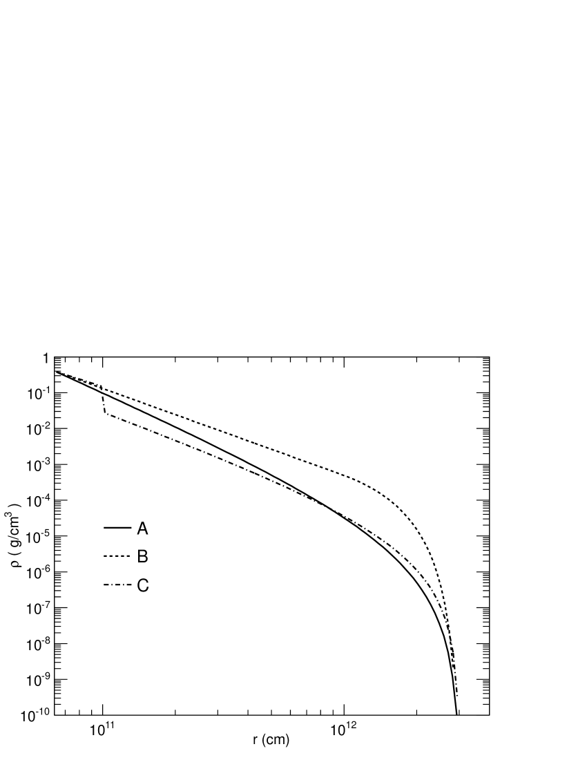
Figure 1: Density profiles of the pressupernova star ( a blue supergiant) of models A, B and C with a radius $R_{*}=3\times 10^{12}$ cm. In these models, the high energy neutrinos are produced at a radius $r_{j}=10^{10.8}$ cm.

Based on above and with the fact that some of the Long GRBs observed are related to SNe (Type Ib/c), we are going to use three possible models as considered in Mena:2006eq . The characteristics of these progenitor models are that they are having an iron core of radius $r_{Fe}\sim 10^{9}$ cm surrounded by a He core extending up to $r_{He}\sim 10^{11}$ cm where the density is $\rho_{He}\sim 10^{-3}\,g/cm^{3}$. In some cases a hydrogen envelope surrounds the He core extending to $r_{H}\gtrsim 10^{13}$ cm with a density of $\rho_{H}\sim 10^{-7}\,g/cm^{3}$ . The presupernova stars which are believed to be the strong contender for the Long GRBs are Type Ic SNe which have lost their hydrogen envelopes as well as most of the He envelope before the explosion. These objects are not interesting from the point of view of neutrino oscillation because their radii are too small to have any appreciable effect. On the other hand, the presupernova stars with the He envelope (Type Ib SNe) and even the H envelope (Type II SNe) intact will be favorable for TeV neutrino production as well as their oscillation in the stellar environment. We consider three different presupernova models as shown in FIG. 1. In all these models the radius of the BSG is taken to be $R_{*}\simeq 3\times 10^{12}$ cm. The jet evolves at a radius $r_{j}\simeq 10^{10.8}$ cm $<r_{He}$ and also the $\gtrsim$ 5 TeV neutrinos are produced at a point between $r_{j}$ and $r_{He}$ so that the jet can acquire relativistic velocity on the surface of the He envelope. The models are:

• Model A

  $$\rho(r)=\rho_{\ast}\times\left(\frac{R_{*}}{r}-1\right)^{3}\frac{\rm g}{\rm cm^{3}}.$$ (33)

  This model represents a star with a radiative envelope. It has a polytropic structure with a polytropic index $n=3$ and the characteristic density $\rho_{\ast}=4.0\times 10^{-6}$ g/cm³. This model is valid only in the region of the star that lies between the point were the jet is produced and the star envelope i.e. $r_{j}\lesssim r\lesssim R_{*}$.

• Model B

  $$\rho(r)=\rho_{\ast}\times\left\{\begin{array}[]{ll}\left(\frac{R_{*}}{r}\right)^{n}&;10^{10.8}\,{\rm cm}<r<r_{b}\\ \left(\frac{R_{*}}{r}\right)^{n}\frac{\left(r-R_{*}\right)^{5}}{\left(r_{b}-R_{*}\right)^{5}}&;r>r_{b}\end{array}\right.\frac{\rm g}{\rm cm^{3}}.$$ (36)

  (37)

  This model is for a BSG with polytropic index $n$=17/7 and with $r_{b}=10^{12}\,{\rm cm}$. The density has a power law behavior with a characteristic density $\rho_{\ast}=3.4\times 10^{-5}$ g/cm³. This profile was obtained from the fit to SN1987A data.

• Model C

  $$\rho(r)=\rho_{\ast}{\cal A}\left(\frac{R_{*}}{r}-1\right)^{n_{eff}}\frac{\rm g}{\rm cm^{3}},$$ (38)

  where the parameters of model C are given as

  $$\left(n_{eff},{\cal A}\right)=\left\{\begin{array}[]{ll}(2.1,\,20)&;10^{10.8}\,{\rm cm}<r<10^{11}\\ (2.5,\,1.0)&;r>10^{11}\,{\rm cm}.\\ \end{array}\right.$$ (41)

  This model has two free parameters $n_{eff}$ and ${\cal A}$ that can be fitted to produce a drop in the density after the helium core. While the parameter ${\cal A}$ can be used to set a density drop at the edge of the helium core, $n_{eff}$ gives the effective polytropic index Matzner:1998mg . The characteristic density here is $\rho_{\ast}=6.3\times 10^{-6}$ g/cm³. The density profiles of all these three models are shown in FIG. 1.

IV Results

We use the neutrino oscillation formalism of OS given in Sec. II and calculate the neutrino oscillation probabilities and fluxes in presupernova star models A, B and C and also on the surface of the Earth after the neutrinos have undergone vacuum oscillation in the intergalactic medium. For all these calculations we take the neutrino energy in the range 100 GeV to 100 TeV , although it may be difficult to produce neutrinos with energy more than 10-20 TeV in the presupernova star environment.

We use the standard neutrino oscillation parameters obtained from different experiments for analysis of our results. The neutrino parameters used are as follows:

$$\Delta m^{2}_{21}=8.0\times 10^{-5}\,eV^{2},\,\,\theta_{12}=33.8^{\circ}\,\,{\rm and}\,\,\theta_{23}=45^{\circ}$$

$$\Delta m^{2}_{32}=3.2\times 10^{-3}\,eV^{2},\,\,\,\theta_{13}=8.8^{\circ}\,\,{\rm and}\,\,\delta_{CP}=0.$$ (43)

We also we take $\theta_{13}=12^{\circ}$ to observe the variation in oscillation probability due to change in this angle.

For the numerical calculation, we divide the distance $(R_{*}-r_{j})$ into small slices, each with a constant density and calculate $U_{f}(L)$ for each individual slices as discussed in Eq.(32). Afterward we use Eq.(23) to calculate the probabilities. We let the high energy neutrinos propagate from the production point at $r_{j}=10^{10.8}$ cm towards the surface of the star $R_{*}$, where we calculate their survival and transition probabilities $P_{\alpha\beta}$ and $P_{{\bar{\alpha}}\bar{\beta}}$, as well as fluxes. We consider two different sets of parameters: $R_{*}=3\times 10^{12}\,{\rm cm}$ and $\theta_{13}=8^{\circ}$ (Set-I); $R_{*}=2.7\times 10^{12}\,{\rm cm}$ and $\theta_{13}=12^{\circ}$ (Set-II); to observe the variation in the probabilities at different depth from the star surface and different $\theta_{13}$.

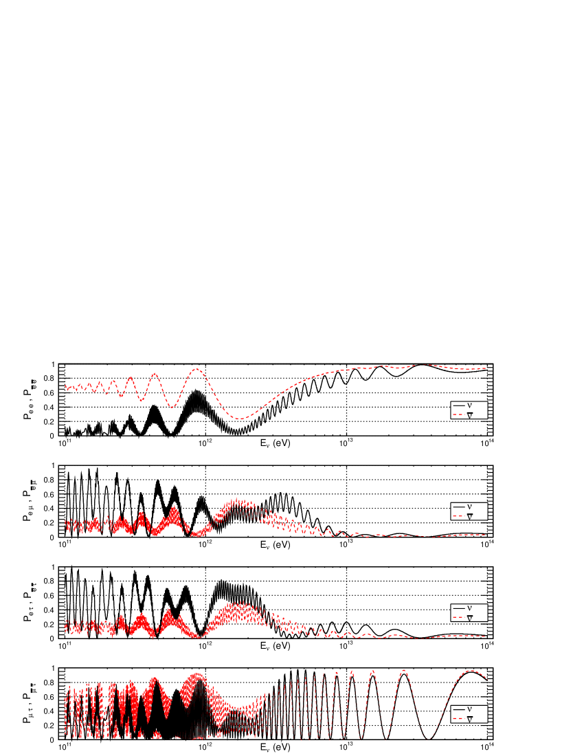
Figure 2: The oscillation probabilities for neutrinos (black solid line) and anti-neutrinos (red dotted line) are plotted as functions of neutrino/anti-neutrino energy $E_{\nu}$ for model A, Set-I where first figure is for $P_{ee}$ and $P_{{\bar{e}}{\bar{e}}}$, second figure is for $P_{e\mu}$ and $P_{\bar{e}\bar{\mu}}$, third figure is for $P_{e\tau}$, $P_{{\bar{e}}{\bar{\tau}}}$ and the fourth one is for $P_{\mu\tau}$ and $P_{{\bar{\mu}}{\bar{\tau}}}$ respectively.

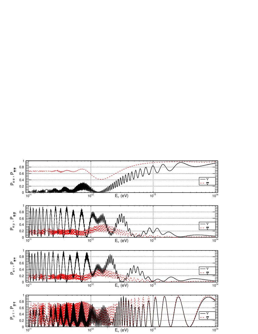
Figure 3: This is same as FIG.2 but for model-B. (See the electronic edition of the Journal for a color version of the figures and the color specification is same as FIG.2).

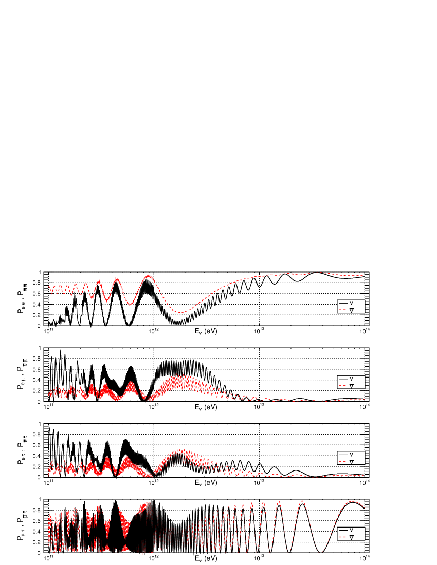
Figure 4: This is same as FIG.2 but for model-C.

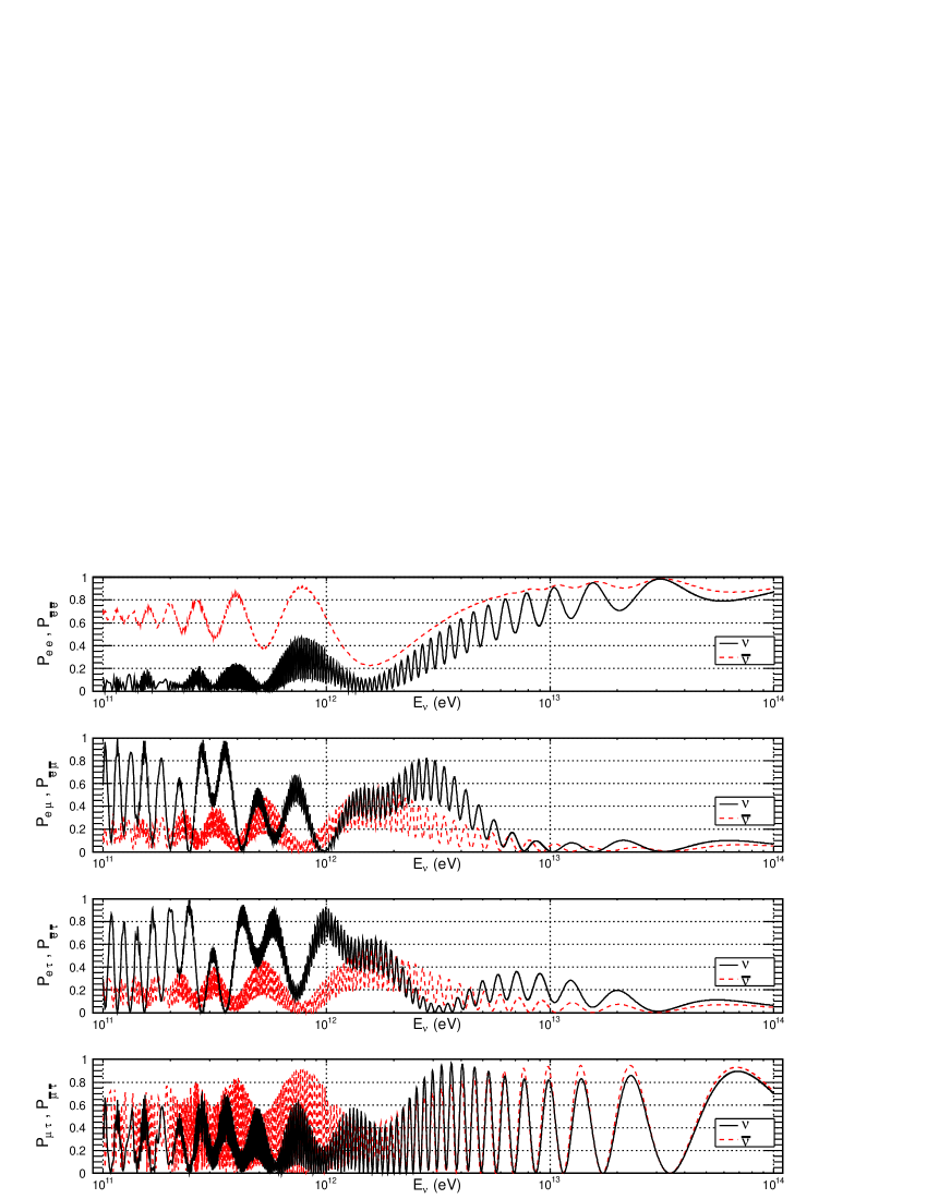
Figure 5: This is same as FIG.2 but for the parameter set-II.

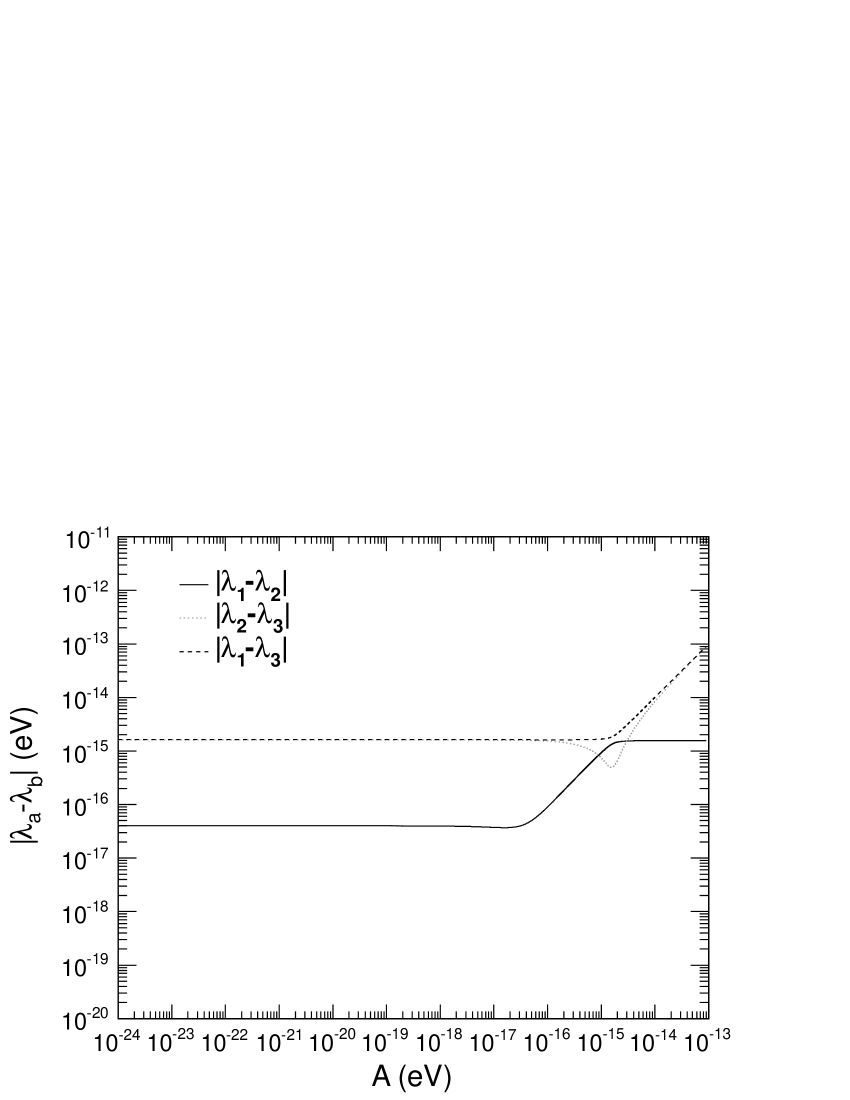
Figure 6: The energy difference is plotted as a function of potential energy A to look for the existence of resonance.

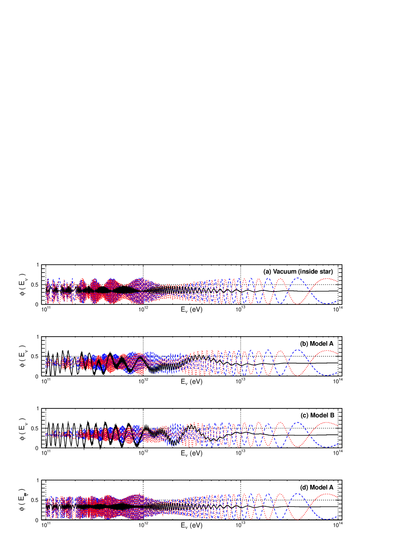
Figure 7: Neutrino and anti-neutrino fluxes on the surface of the star. In (a), (b) and (c) black solid line is for $\Phi_{\nu_{e}}$, blue dashed lines is for $\Phi_{\nu_{\mu}}$, and red dotted line is for $\Phi_{\nu_{\tau}}$. In (d) black solid curve, blue dashed curve and red dotted curve are for $\Phi_{{\bar{\nu}}_{e}}$, $\Phi_{{\bar{\nu}}_{\mu}}$ and $\Phi_{{\bar{\nu}}_{\tau}}$ respectively.

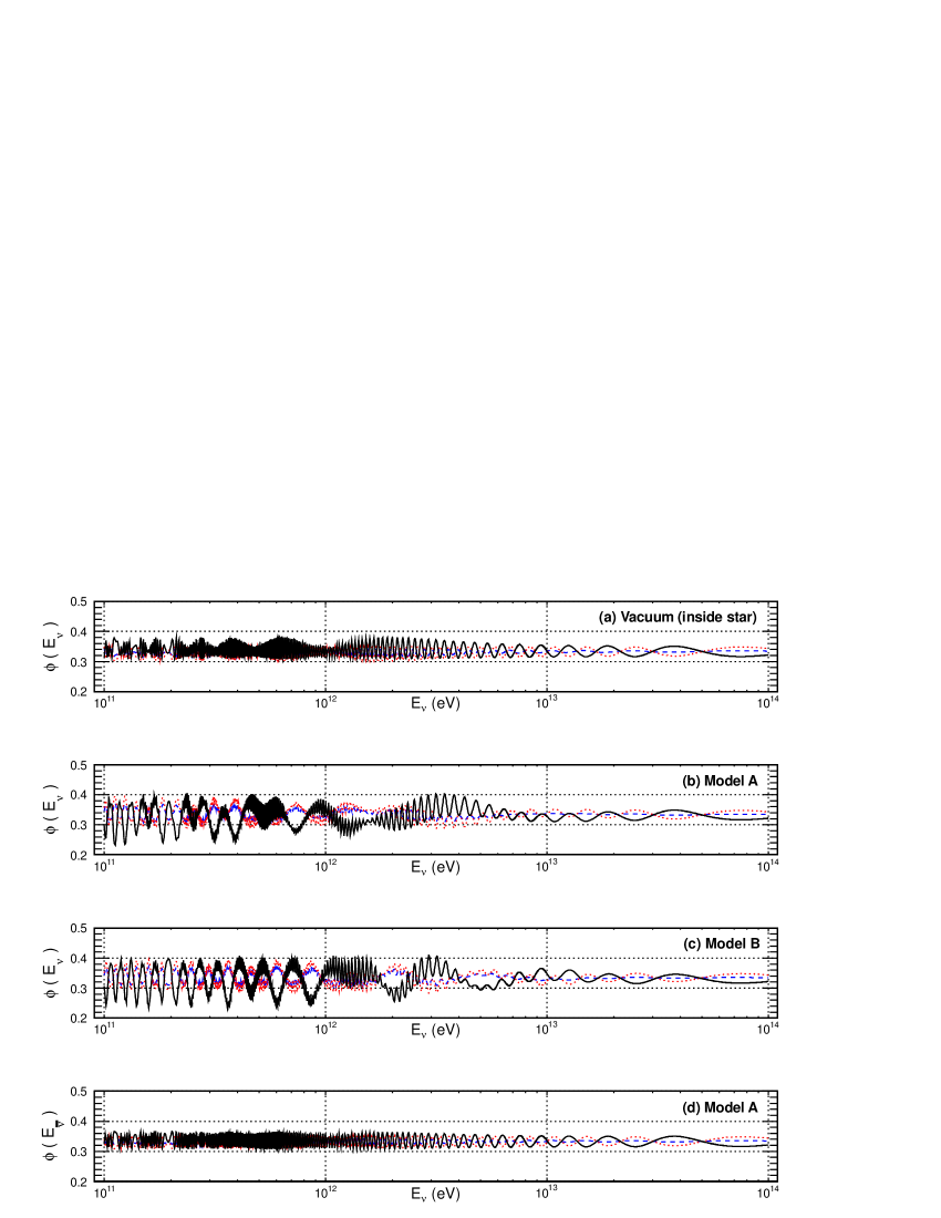
Figure 8: Same as FIG.7 but the flux is calculated on the surface of the Earth.

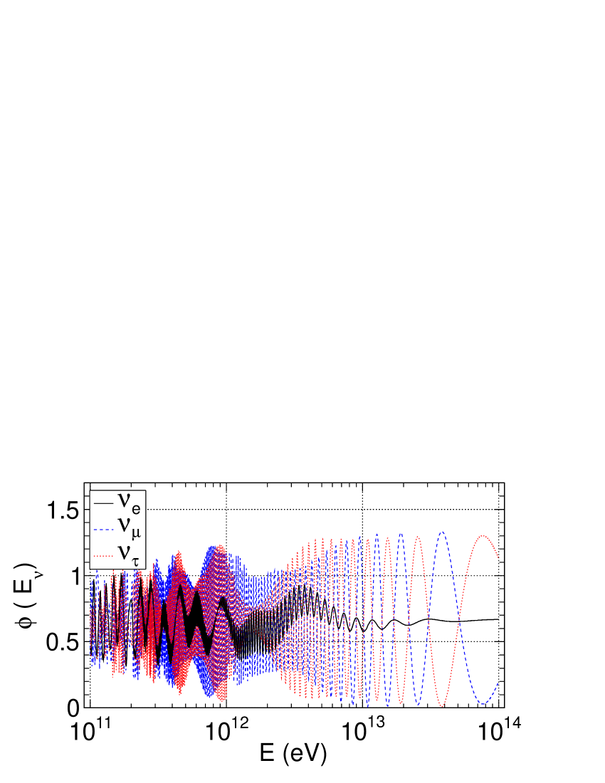
Figure 9: The total flux (neutrino+anti-neutrino) on the surface of the star, where the black solid, blue dashed and red dotted curves are for $\Phi_{\nu_{e}}$, $\Phi_{\nu_{\mu}}$ and $\Phi_{\nu_{\tau}}$ respectively.

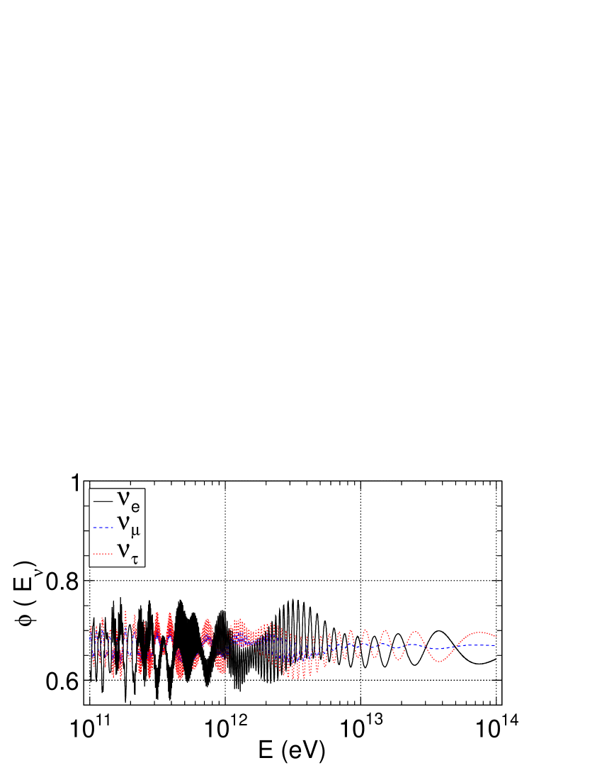
Figure 10: The total flux (neutrino+anti-neutrino) on the surface of the Earth, where the black solid, blue dashed and red dotted curves are for $\Phi_{\nu_{e}}$, $\Phi_{\nu_{\mu}}$ and $\Phi_{\nu_{\tau}}$ respectively.

The survival and transition probabilities of $\nu$ and ${\bar{\nu}}$ for the parameter Set-I, for models A, B and C are shown in FIGs. 2, 3 and 4 respectively. We have also plotted the variation in oscillation probabilities for Set-II in FIG. 5. We observe that for a given neutrino energy $E_{\nu}$, $P_{{\bar{e}}{\bar{e}}}$ is always above $P_{ee}$ and the probabilities are highly oscillatory for $E_{\nu}\lesssim 10^{12}$ eV. For $E_{\nu}\gtrsim 2\times 10^{12}$ eV, both $P_{ee}$ and $P_{{\bar{e}}{\bar{e}}}$ increase towards unity. While the increase in $P_{{\bar{e}}{\bar{e}}}$ is smooth, the increase in $P_{ee}$ is accompanied by a rapid oscillation, as shown in these figures. By reducing the $R_{*}$ to $2.7\times 10^{12}$ cm and $\theta_{13}=12^{\circ}$ i.e. Set-II (FIG. 5 ), we observe that, although there is variation of probability on the surface, the overall behavior is exactly the same as the parameter Set-I shown in FIG.2. So for our further discussion we only consider the parameter Set-I for the analysis of our results. All the transition probabilities $P_{e\mu}$, $P_{e\tau}$, $P_{\mu\tau}$ $P_{\bar{e}\bar{\mu}}$, $P_{{\bar{e}}{\bar{\tau}}}$ and $P_{{\bar{\mu}}{\bar{\tau}}}$ are highly oscillatory in all the energy ranges (mostly $\lesssim 10^{13}$ eV). For neutrino energy $E_{\nu}>3\times 10^{12}$ eV the transition probabilities $P_{e\mu}$, $P_{e\tau}$, $P_{\bar{e}\bar{\mu}}$ and $P_{{\bar{e}}{\bar{\tau}}}$ go to zero, which shows that the medium has almost no effect on high energy neutrinos. On the other hand $P_{\mu\tau}$ and $P_{{\bar{\mu}}{\bar{\tau}}}$ are highly oscillatory in this energy range. The $P_{e\mu}$ and $P_{e\tau}$ are different from each other due to the matter effect. Comparison of $P_{\bar{e}\bar{\mu}}$ and $P_{{\bar{e}}{\bar{\tau}}}$ shows that they oscillate with same amplitude, but are out of phase by $180^{\circ}$. The transition probabilities $P_{\mu\tau}$ and $P_{{\bar{\mu}}{\bar{\tau}}}$ are different for energies below $\sim 3\times 10^{12}$ eV, but are almost the same above this energy for all the models A, B, and C (last of FIGs. 2, 3, 4 and 5) which is due to the negligible medium effect on the high energy neutrinos.

The energy eigenvalues of the neutrinos in the matter are $\lambda_{a}$ and the energy difference $|\lambda_{a}-\lambda_{b}|$ is related to the effective mass square difference

$$|\lambda_{a}-\lambda_{b}|=\frac{|{\tilde{\Delta m}}^{2}_{ab}|}{2E_{\nu}}.$$ (44)

In FIG.6, for the illustrative purpose, we have taken $E_{\nu}=1$ TeV with parameter Set-I and model-A to show the resonance position as a function of matter potential A. It shows that there is only one resonance position around $A\simeq 2\times 10^{-15}$ eV (between $|\lambda_{1}-\lambda_{2}|$ and $|\lambda_{1}-\lambda_{3}|$). By taking $E_{\nu}=10$ TeV we found that the resonance position is almost the same. The anti-neutrinos will not satisfy the resonance condition because of the change in the sign of the potential $A$ in $\lambda_{a}$.

In the mildly relativistic jet internal shocks can develop and accelerate protons to very high energies. These protons would interact with the $\sim$ keV thermal X-ray photons to produce TeV neutrinos via the process $p+\gamma\rightarrow\Delta^{+}\rightarrow n+\pi^{+}\rightarrow n+\mu^{+}+\nu_{\mu}\rightarrow n+e^{+}+\nu_{\mu}+\nu_{e}+{\bar{\nu}_{\mu}}$. In the above process the standard neutrino flux ratio at the production point is $\Phi^{0}_{\nu_{e}}:\Phi^{0}_{\nu_{\mu}}:\Phi^{0}_{\nu_{\tau}}=1:2:0$ ($\Phi^{0}_{\nu_{\alpha}}$ corresponds to the sum of neutrino and anti-neutrino flux at the source). The flux observed at a distance is given by

$$\Phi_{\nu_{\alpha}}=\sum_{\beta}\Phi^{0}_{\nu_{\beta}}P_{\alpha\beta},\,\,\alpha,\beta=e,\,\mu,\,\tau.$$ (45)

Using models A, B and C, we have calculated the normalized fluxes of neutrinos and anti-neutrinos on the surface of the presupernova star as well as on the surface of the Earth, which are shown in FIGs. 7 and 8. In these figures, (a) is the flux calculation in vacuum (where the matter potential $A=0$ inside the star) and the (b), (c) are for models A, B and (d) is for anti-neutrino fluxes for model A respectively. The comparison of the vacuum oscillation i.e. (a) with the rest i.e. (b), (c) and (d), shows that for $E_{\nu}\gtrsim 6\times 10^{12}$ eV both the fluxes are the same, which signifies that above this energy the matter effect is negligible and below this energy the normalized flux is oscillatory and energy dependent. Also the comparison of fluxes of neutrinos (b) and anti-neutrinos (d) in model A below $E_{\nu}\gtrsim 6\times 10^{12}$ eV are different.

In FIGs. 9 and 10 we have shown the total flux (neutrino and anti-neutrino) of $\nu_{e}$, $\nu_{\mu}$ and $\nu_{\tau}$ on the surface of the star and on Earth. It can be observed that the fluxes of different neutrinos are different on the surface of the star. For $E_{\nu}\lesssim 4\times 10^{12}$ eV, the fluxes on Earth are also different but above this energy the flux ratio is close to 1:1:1.

V Summary

It is observed that only a very small fraction of core collapse SNe are responsible for GRBs and majority of them fail to produce $\gamma$-rays. This majority class are efficient emitters of TeV neutrinos which can be observable in IceCube. Here we study the matter effect of the presupernova star on the propagation of these high energy neutrinos by taking into account all the three active flavors and using the formalism developed by OS. We observed that the neutrino oscillation within the presupernova star depends on the neutrino energy and alter their flux on the surface of the star. We also calculated the fluxes of these neutrinos on the Earth after they travelled the intergalactic medium (vacuum oscillation) and found that low energy neutrinos $E_{\nu}\lesssim 4$ TeV have different fluxes whereas above this energy the flux ration is close to 1:1:1. So, possible detection of high energy neutrinos with $E_{\nu}\lesssim 10$ TeV by IceCube can be important due to the change in their fluxes when they propagate through the choked environment of the presupernova stars. Also detection of these neutrinos might shed more light on the type of progenitors and the acceleration mechanisms of the high energy cosmic rays. As application and continuation of the present work, the calculation of the neutrino induced muon (track) to electron (shower) ratio in IceCube is in preparation.

S.S. is thankful to Departamento de Fisica de Universidad de los Andes, Bogota, Colombia, for their kind hospitality during his several visits. We thank Karla Patricia Varela for helpful discussions. This work is partially supported by DGAPA-UNAM (Mexico) Project No. IN103812.

References

- (1) T. J. Galama, P. M. Vreeswijk, J. van Paradijs, C. Kouveliotou, T. Augusteijn, O. R. Hainaut, F. Patat and H. Bohnhardt et al., Nature 395, 670 (1998) [astro-ph/9806175].
- (2) P. A. Mazzali, J. S. Deng, N. Tominaga, K. Maeda, K. .Nomoto, T. Matheson, K. S. Kawabata and K. Z. Stanek et al., Astrophys. J. 599, L95 (2003) [astro-ph/0309555].
- (3) B. Thomsen, J. Hjorth, D. Watson, J. Gorosabel, J. P. U. Fynbo, B. L. Jensen, M. I. Andersen and T. H. Dall et al., Astron. Astrophys. 419, L21 (2004) [astro-ph/0403451].
- (4) M. Della Valle, D. Malesani, S. Benetti, V. Testa, M. Hamuy, L. A. Antonelli, G. Chincarini and G. Cocozza et al., Astron. Astrophys. 406, L33 (2003) [astro-ph/0306298].
- (5) S. E. Woosley and J. S. Bloom, Ann. Rev. Astron. Astrophys. 44, 507 (2006) [astro-ph/0609142].
- (6) B. Zhang, B. B. Zhang, F. J. Virgili, E. W. Liang, D. A. Kann, X. F. Wu, D. Proga and H. J. Lv et al., Astrophys. J. 703, 1696 (2009) [arXiv:0902.2419 [astro-ph.HE]].
- (7) E. Waxman and J. N. Bahcall, Phys. Rev. Lett. 78, 2292 (1997); E. Waxman and J. N. Bahcall, Phys. Rev. D 59, 023002 (1999).
- (8) E. Berger, S. R. Kulkarni, D. A. Frail and A. M. Soderberg, Astrophys. J. 599, 408 (2003);
- (9) P. Mészáros and E. Waxman, Phys. Rev. Lett. 87, 171102 (2001).
- (10) S. Razzaque, P. Mészáros and E. Waxman, Phys. Rev. Lett. 93, 181101 (2004) [Erratum-ibid. 94, 109903 (2005)].
- (11) T. J. Galama et al., Nature, 395, 670 (1998); S. Campana et al., Nature 442, 1008 (2006).
- (12) E. Liang et al., Astrophys. J. 662, 1111 (2007); K. Murase et al., Astrophys. J. 651, L5 (2006); N. Gupta and B. Zhang, AstroParticle. Phys. 27, 386 (2007)
- (13) S. Razzaque, P. Meszaros and E. Waxman, Phys. Rev. D 68, 083001 (2003) [astro-ph/0303505].
- (14) S. Razzaque, P. Meszaros and E. Waxman, Mod. Phys. Lett. A 20, 2351 (2005) [astro-ph/0509729].
- (15) S. Sahu and B. Zhang, Res. Astron. Astrophys. 10, 943 (2010) [arXiv:1007.4582 [hep-ph]].
- (16) V. D. Barger, K. Whisnant, S. Pakvasa and R. J. N. Phillips, Phys. Rev. D 22, 2718 (1980).
- (17) C. W. Kim and W. K. Sze, Phys. Rev. D 35, 1404 (1987).
- (18) H. W. Zaglauer and K. H. Schwarzer, Z. Phys. C 40, 273 (1988).
- (19) S. T. Petcov, Phys. Lett. B 191, 299 (1987).
- (20) H. Lehmann, P. Osland and T. T. Wu, Commun. Math. Phys. 219, 77 (2001) [hep-ph/0006213].
- (21) P. Osland and T. T. Wu, Phys. Rev. D 62, 013008 (2000) [hep-ph/9912540].
- (22) T. Ohlsson and H. Snellman, J. Math. Phys. 41, 2768 (2000) [Erratum-ibid. 42, 2345 (2001)] [hep-ph/9910546].
- (23) T. Ohlsson and H. Snellman, Phys. Lett. B 474, 153 (2000) [hep-ph/9912295].
- (24) T. Ohlsson and H. Snellman, Eur. Phys. J. C 20, 507 (2001) [hep-ph/0103252].
- (25) A. I. MacFadyen, S. E. Woosley and A. Heger, Astrophys. J. 550, 410 (2001) [astro-ph/9910034].
- (26) C. D. Matzner and C. F. McKee, Astrophys. J. 510, 379 (1999) [astro-ph/9910034].
- (27) T. Shigeyama and K. Nomoto, C. D. Matzner and C. F. McKee, Astrophys. J. 360, 242 (1990).
- (28) D. Arnett, Astrophys. J. 383, 295 (1991).
- (29) R. A. Chevalier and N. Soker, Astrophys. J. 341, 867 (1989).
- (30) O. Mena, I. Mocioiu and S. Razzaque, Phys. Rev. D 75, 063003 (2007) [astro-ph/0612325].