Effect of charge on the dynamics of an acoustically forced bubble

Abstract

The effect of charge on the dynamics of a gas bubble undergoing forced oscillations in a liquid due to incidence of an ultrasonic wave is theoretically investigated. The limiting values of the possible charge a bubble may physically carry are obtained. The presence of charge influences the regime in which the bubble’s radial oscillations fall. The extremal compressive and expansive dimensions of the bubble are also studied as a function of the amplitude of the driving pressure. It is shown that the limiting value of the bubble charge is dictated both by the minimal value reachable of the bubble radius as well as the amplitude of the driving ultrasound pressure wave. A non-dimensional ratio ${\zeta}$ is defined that is a comparative measure of the extremal values the bubble can expand or contract to and find the existence of an unstable regime for ${\zeta}$ as a function of the driving pressure amplitude, $P_{s}$. This unstable regime is gradually suppressed with increasing bubble size. The Blake and the upper transient pressure thresholds for the system are then discussed.

I Introduction

The study of bubble dynamics and cavitation has a long and interesting history in the scientific literature. One of the earliest works was that of Lord Rayleigh rayleigh in his study of cavitation phenomena, motivated by the need to understand and minimize the damage to ships’ propellors due to cavitation (the low pressure on the surface of the propeller blades causes the liquid in contact with the surface to spontaneously form unstable bubble clouds which often self-organize into dendritic structuresneppiras . These bubble clouds implode with enormous force resulting in serious damages to the propeller).
Cavitation, bubble formation and dynamics are present in different instances and situations. Analyses and studies of the phenomena have been motivated by and have explained very distinct natural, practical phenomena. Small amplitude oscillations of a gas bubble in a liquid were studied by Minnaert minnaert . His work showed the important contribution of radial oscillations of entrailed air bubbles in the sound heard from running water.
In nature, the snapping shrimp uses rapid closure of its claws to generate cavitating bubbles which stun its prey versluis . Bubble formation and kinetics contribute to fluid flow in biological systems in blood and cells in the micron scale marmot . In the presence of incident ultrasound waves, bubbles can also enhance the rate of chemical reactions suslick ; masonbook . Bubble formation and cavitation can be recreated under controlled conditions in the laboratory by subjecting a liquid in a container to a standing ultrasonic wave, setting up a pressure field within the liquid. When the driving pressure amplitude of the sonic field becomes larger than the ambient pressure, the pressure in the liquid becomes negative. When this pressure exceeds the vapour pressure of the liquid, local evaporation is caused. The liquid ‘breaks’ up forming tiny micron size cavitation bubble clouds, which implode violently within a very short period of time. Frenzel and Schultes demonstrated that these cavitation clouds emitted low intensity visible light frenzel . This phenomenon, wherein light is emitted by a gas bubble in a liquid due to its rapid expansion and collapse when ultrasound is incident on it, is known as sonoluminescence. This has also contributed to an extensive study of bubble dynamics in the context of sonoluminescence. Several other studies have followed in the literature, including those of Gaitan and others gaitan1 ; gaitan2 ; gaitan3 ; barberPutterman . The radial oscillations of gas bubbles in a liquid that are caused due to incident acoustic waves cannot be described trivially. These are a type of driven nonlinear oscillations that can greatly depend on initial conditions and can be chaotic in nature. This has been shown conclusively (see, for example, brennerRMP ; lauterborn ; smereka ; lauterborn2 ; parlitz and references therein). Reviews may be found in, for example,  masonbook ; brennerRMP ; brennenbook .

The presence of electric charge on bubbles in fluids has been reported in the experimental literature.  mctaggart ; alty ; alty2 ; akulichev ; shiran .
In this paper we use the Rayleigh-Plesset equation modified by Parlitz, et al., further modified to take into account the presence of charge on the bubble, and study the effects of charge, driving frequency and amplitude of the ultrasonic driving field on the dynamics of the bubble, with the specific heat ratio being taken as 5/3 in our calculations, consistent with the gas in the bubble being a monatomic ideal, inert gas under adiabatic conditions. In Section II, we describe the model used; the natural frequency of oscillation of the bubble is obtained and the phase plots show that the maximal radial velocity for the charged bubble greatly exceeds that of the neutral bubble. In Section III the Blake radius and threshold for the charged bubble are calculated. This is followed by a discussion of Rayleigh collapse and the influence of driving pressure amplitude in Section IV. We show that for a bubble of given ambient radius $R_{0}$, there exists a cut-off value for the maximum charge it can carry, which is dictated by the van der Waals hard-core radius. In Section V we introduce a new dimensionless ratio $\zeta$ as a measure of the maximum and minimum radius a bubble can achieve under acoustic driving. This when plotted as a function of pressure amplitude clearly captures the positions of the Blake threshold and the upper critical transient pressure threshold for acoustic cavitation, and their distinct dependence on the pressure amplitude, driving frequency and bubble charge. Bubbles that are present in various systems can carry a non-zero charge. Hence, a proper understanding of their behavior and dependence on pressure, driving frequency, ambient radius and other parameters, is essential. This is the subject of investigation of this paper. The results obtained in our work therefore become very useful in the context of medical uses of acoustic cavitation and ultrasound for diagnostic and therapeutic purposes.

II The Model

We shall briefly describe the model and the set of equations being used to describe the radial oscillations of gas bubbles in liquids. Various models have investigated distinct, disparate limits of bubble-collapse. The original work of Rayleigh assumed the surrounding liquid to be inviscid and incompressibile rayleigh . Plesset and others  plesset1 ; plesset2 ; noltingkNeppiras have included viscosity, surface tension etc. Keller and Kolodner used the same expression but with a modification for accounting for acoustic radiation by the bubble by considering the liquid as slightly compressible kellerKolodner . Keller and Miksis further included all these modifications – of viscosity, surface tension, the incident sound wave and acoustic radiation, in one model to obtain a modified equation kellerMiksis .

The model we use to describe the system is based on the earlier equations of Prosperetti, Parlitz and Keller and Miksis and others parlitz ; kellerMiksis ; plessetProsperetti ; prosperetti-etal and which are modifications of the Rayleigh-Plesset equations rayleigh ; plesset1 ; plesset2 .

The system we consider is that of a bubble suspended in a liquid and that has some net charge. The presence of charge on a bubble is not speculative. As mentioned earlier, electric charge has been found on bubbles under acoustic forcing. Various reasons could cause charge to be present on the bubble, e.g., the migration of ionic charges in the liquid onto the bubble surface, although the exact mechanism has been debated. See, for example, the work of Alty alty ; alty2 and Akulichev akulichev . That gas bubbles in water can carry a charge has been clearly demonstrated long back alty ; alty2 . Indeed, it had been shown earlier mctaggart that air and other gas bubbles in water become negatively charged. More recently, this has been shown by Shiran and Watmough shiran . Therein, bubbles placed in an electric field are clearly demonstrated to veer towards one of the electrodes.

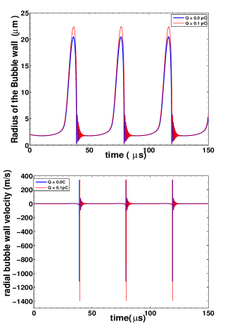
Figure 1: Plots of a bubble’s radius (above) & radial velocity (below) as a function of time ($P_{s}=1.35P_{0}$, $R_{0}=2\mu m$, $\nu=25$ kHz). The curve for the charged bubble (with charge 0.1 pC) reaches a larger magnitude (for both radius and velocity plots) than for the neutral bubble. (Color Online).

Other work on the presence of charge on bubbles in different situations include that done by Bunkin and Bunkin bunkin .
The study of the dynamics of charged gas bubbles in fluids is important because such systems find various applications, including in medicine – a widely used one being in the medical application of ultrasound. While it has been overlooked in several models, various investigations of charged bubbles have appeared in the literature in different contexts. These include, for example, zharov . Their work is however of very limited scope since they consider the specific case for which the polytropic index $\Gamma$ takes the value 4/3 and for this case it turns out that the terms containing the charge mutually cancel out in the Rayleigh-Plesset equation.

We take $\Gamma=5/3$ consistent with taking the heat transfer across the bubble to be an adiabatic process. For the sake of simplicity, we assume the charge to be strictly limited to, and uniformly distributed on, the surface of the bubble.
The surface charge density of the bubble thus changes as the bubble expands and contracts along with the acoustic forcing being externally applied to it. As mentioned above, we use a modified form of the Rayleigh-Plesset equation, one introduced by Parlitz, et al. parlitz , which is equivalent in first order in ($1/c$) to that of Keller and Miksis kellerMiksis ($c$ being the velocity of sound) and which includes, approximately, the sound radiation which is the most significant contribution to damping at higher amplitudes of bubble excitation. In the presence of charge, this equation describing the dynamical evolution of the bubble radius $R$ in time gets further modified.

Considering the charged bubble as a non-conducting charged shell with a constant charge $Q$, the electrostatic pressure can be calculated as has been done by Akulichev, Atchley and others akulichev ; atchley ; bunkin ; zharov . The presence of charge $Q$ (or surface charge density $S$) causes the inclusion of an electrostatic pressure term $2\pi S^{2}/\epsilon=Q^{2}/(8\pi\epsilon R^{4})$ into the equation (see e.g., zharov , also ashok ):

$$\left[\left(1-\frac{\dot{R}}{c}\right)R+\frac{4\eta}{c\rho}\right]\ddot{R}=\frac{1}{\rho}\left(P_{0}-P_{v}+\frac{2\sigma}{R_{0}}-\frac{Q^{2}}{8\pi\epsilon R_{0}^{4}}\right)$$

$$\times\left(\frac{R_{0}}{R}\right)^{3\Gamma}\left(1+\frac{\dot{R}}{c}(1-3\Gamma)\right)-\frac{\dot{R}^{2}}{2}\left(3-\frac{\dot{R}}{c}\right)$$

$$+\frac{Q^{2}}{8\pi\rho\epsilon R^{4}}\left(1-\frac{3\dot{R}}{c}\right)-\frac{2\sigma}{\rho R}-\frac{4\eta}{\rho}\left(\frac{\dot{R}}{R}\right)$$

$$-\frac{1}{\rho}(P_{0}-P_{v}+P_{s}\textrm{sin}(\omega t))\left(1+\frac{\dot{R}}{c}\right)-\frac{R}{\rho c}P_{s}\omega\textrm{cos}(\omega t)$$

where $R_{0}$ is the ambient bubble radius, $P_{0}$ is the static pressure of the, $P_{s}$ and $\omega=2\pi\nu$ denote respectively the amplitude and angular frequency of the driving sonic field, $P_{v}=2.34$kPa is the vapour pressure of the gas, $\sigma$, $\rho$ and $\eta$ denote respectively the surface tension, density and viscosity of the liquid surrounding the bubble. $c$ is the velocity of sound in the liquid. In this work, for the purpose of the numerical results reported, we consider water to be the liquid, with $\rho=998kg/m^{3}$, $\eta=10^{-3}Ns/m^{2}$, $c=1500m/s$, $P_{0}=101kPa$, $\sigma=0.0725N/m$, $\epsilon=85\epsilon_{0}$ where $\epsilon_{0}$ is the permittivity of vacuum.
The presence of charge $Q$ modifies the influence of surface tension, reducing its effective value (the effective surface tension changes from $\sigma$ for the uncharged case to $\sigma-Q^{2}/(16\pi\epsilon R_{0}^{3})$) and induces several interesting changes to the dynamics of bubble oscillations.
When a pressure wave is incident on a bubble in a liquid, the difference in pressure can cause expansion and rapid collapse of the bubble, this being followed immediately after by further, smaller oscillations which are termed as afterbounces. This entire sequence of a maximal expansion of the bubble followed by collapse and afterbounces, is repeated in each cycle when we have sinusoidal forcing by ultrasound. When a bubble is in the sonoluminescent regime, light emission occurs shortly after the bubble’s violent contraction to a minimal radius, before the onset of aftebounces and repetition of this sequence. Details of the phenomenon of sonoluminescence may be found in, for example, the review articles brennerRMP ; barber . We recast eqn.(1) in dimensionless form for ease of evaluation by redefining the radius $R$ through $r=R/R_{0}$ and time $t$ through $\tau=\omega t$, $r$ and $\tau$ being the new dimensionless radius and time variables. Using the static pressure $P_{0}$ as the reference pressure we also define the dimensionless quantities , $P_{*v}=P_{v}/P_{0}$ and $P_{*s}=P_{s}/P_{0}$. Using an overdot to now denote differentiation with respect to $\tau$, the dimensionless time variable (rather than with respect to $t$), eqn.(1) can be written in dimensionless form as

$$\left(1-\frac{\dot{r}}{c_{*}}\right)r\ddot{r}+F\ddot{r}+\frac{\dot{r}^{2}}{2}\left(3-\frac{\dot{r}}{c_{*}}\right)$$

$$= G\left(1-P_{*v}+M\right)\left(\frac{1}{r}\right)^{3\Gamma}\left(1+\frac{\dot{r}}{c_{*}}(1-3\Gamma)\right)$$

$$+ \frac{C}{r^{4}}\left(1-\frac{3\dot{r}}{c_{*}}\right)-S\frac{1}{r}-Fc_{*}\left(\frac{\dot{r}}{r}\right)$$

$$- G\left(1-P_{*v}+P_{*s}\sin(\tau)\right)\left(1+\frac{\dot{r}}{c_{*}}\right)-G\frac{rP_{*s}}{c_{*}}\cos(\tau)$$

where

$$c_{*}=\frac{c}{R_{0}\omega};\,\,\,\,F=\frac{4\eta}{\rho R_{0}c};\,\,\,\,G=\frac{P_{0}}{R_{0}^{2}\omega^{2}\rho};$$

$$M=\frac{1}{P_{0}}\left(\frac{2\sigma}{R_{0}}-\frac{Q^{2}}{8\pi\epsilon R_{0}^{4}}\right)$$

$$C=\frac{Q^{2}}{8\pi\epsilon R_{0}^{6}{\omega}^{2}\rho};\,\,\,\,S=\frac{2\sigma}{\rho R_{0}^{3}\omega^{2}}$$

are all dimensionless constants.
This form is used when solving the equation numerically. In what follows, we will use the dimensional form of the equation everywhere. It should be understood though, that data points shown in all the graphs have been obtained after numerical evaluation of the corresponding dimensionless quantities, followed by rescaling by the appropriate multiplicative factors to obtain the variables in physically realizable units.
Figure 1 shows a plot of the radius of the bubble as a function of time, obtained by solving equation (II), for charge present on, as well as absent from, the bubble surface.
For a given driving frequency of the pressure wave, the maximum radius attainable by the bubble increases with charge present. Conversely, the minimum radius achievable also reduces with increasing charge. These are as expected.
The difference in behaviour can be seen more emphatically in a plot of the bubble’s radial velocity as a function of time (in Figure 1). In the plot shown, in the presence of charge, the maximum velocity increases to more than five quarters of its uncharged value. This gives us a picture of the dynamics consistent with the time-series of the bubble radius, namely, that the bubble oscillations become more violent in the presence of charge, causing the bubble to expand to a greater extent and contract to a lesser minimal radius than in the absence of any surface charge.

The phase portrait for the system is shown in Fig.2 for both a charged as well as uncharged bubble.

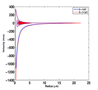
Figure 2: $\dot{R}$ vs. $R$ phase plots for charged and uncharged bubble. The charged case ($Q=0.1$ pC) spans larger magnitudes of velocity and radius. $R_{0}=2\mu m,P_{s}=1.35P_{0},\nu=25kHz$. (Color Online).

The phase plot for the charged bubble is larger than that of the uncharged case, reaching larger values of the magnitudes of both radius and velocity. One can intuitively expect this. During the expansion part of the cycle, the charges present on the bubble surface move away from each other as the bubble expands, decreasing the surface charge density of the bubble wall. The change in the value of the maximal radius of the bubble due to the presence of charge, though present, is small. Due to the decrease in surface tension, we would expect the radius of the bubble to grow slightly more than in the case when there is no charge present. On the other hand, during the collapse, the surface charge density increases rapidly. It is in this regime that we would expect to see most clearly the effects of charge on the dynamics of the bubble. Since the maximum radius attained is larger, the collapse would be expected to be more violent resulting in a higher peak velocity of the bubble wall at the moment of collapse and lower minimum radius attained.

The natural frequency of bubble oscillations of small amplitude may be found by assuming that the sound field can be introduced through a perturbation of amplitude $\alpha$ which is small plessetProsperetti . Then by assuming that the bubble oscillates about its equilibrium radius $R_{0}$, one can express its radius at time $t$ as

$$R=R_{0}(1+x(t)),$$ (3)

where $x(t)$ is a small quantity of order $\alpha$. Substituting Eqn.(3) in the unforced Rayleigh - Plesset equation and linearising it, we obtain:

$$\ddot{x}+\beta\dot{x}+\omega_{0}^{2}x=0,$$ (4)

where the damping coefficient $\beta$ and the natural frequency of the oscillator are given by

$$\beta = \frac{1}{\rho cR_{0}\left(1+\frac{4\eta}{c\rho R_{0}}\right)}\left(4\phi/R_{0}^{5}+\frac{3Q^{2}}{8\pi\epsilon R_{0}^{4}}+\frac{4\eta c}{R_{0}}\right)$$

$$\omega_{0}^{2} = \frac{1}{\rho R_{0}^{2}\left(1+\frac{4\eta}{c\rho R_{0}}\right)}\left(5\phi/R_{0}^{5}-\frac{2\sigma}{R_{0}}+\frac{4Q^{2}}{8\pi\epsilon R_{0}^{4}}\right)$$ (5)

where only terms linear in $x$ and its derivatives have been retained. In eqns.(5), the quantity $\phi$ defined as

$$\phi/R_{0}^{5}=(P_{0}-P_{v}+\frac{2\sigma}{R_{0}}-\frac{Q^{2}}{8\pi\epsilon R_{0}^{4}}).$$ (6)

is the equilibrium gas pressure in the bubble.
The solutions to the damped equation eqn.(4) represent small amplitude oscillations. Substituting the values of the various parameters in eqns.(5) yields a natural frequency $\omega_{0}$ for a micron-sized bubble that is in the MHz range, in conformity with observations in the literature.

III The Blake threshold

The growth of a bubble can be determined by various threshold conditions apfel . One is the well-known Blake threshold for mechanical growth of a gas bubble. The Blake threshold corresponds to the minimum acoustic pressure $P_{s}=P_{Blake}$ exceeding which will result in the explosive growth of the bubble, culminating in cavitation. Blake threshold calculations are made under the assumption that the pressure fields are quasistatic in nature, and the surface tension dominates over viscous and inertial contributions.

Another threshold that is important is the transient cavitation threshold. This is the minimum acoustic pressure required for the forced oscillating bubble to collapse violently after its maximal expansion at radial velocities at least equalling the speed of sound.
In this section we calculate and discuss the Blake cavitation threshold for the bubble. Further discussion and results related to the upper transient cavitation threshold will be presented in Section V.

One other threshold condition is that determining the diffusion of a gas into the liquid causing bubble expansion, which is determined by factors including the natural resonance frequency of the bubble, the acoustic forcing frequency, the gas saturation coefficient, surface tension, specific heat ratio and the ambient radius of the bubble apfel . We do not discuss this threshold, known as the rectified diffusion threshold, in this work.
The pressure of the liquid on the outer surface of the bubble wall $p_{L}$ may be written down:

$$p_{L}(R(t))=p_{i}(t)-\frac{2\sigma}{R}+\frac{Q^{2}}{8\pi\epsilon R^{4}}-\frac{4\eta\dot{R}}{R}$$ (7)

where the pressure inside the bubble $p_{i}(t)$ comprises of pressure of the gas and the vapour pressure $P_{v}$:

$$p_{i}=(P_{0}-P_{v}+\frac{2\sigma}{R_{0}}+\frac{Q^{2}}{8\pi\epsilon R^{4}})\left(\frac{R_{0}}{R}\right)^{3\Gamma}+P_{v}$$ (8)

The net pressure on the bubble wall from the surrounding liquid is zharov :

$$P = \Big{(}P_{0}-P_{v}+\frac{2\sigma}{R_{0}}-\frac{Q^{2}}{8\pi\epsilon R_{0}^{4}}\Big{)}{\Big{(}\frac{R_{0}}{R}\Big{)}}^{3\Gamma}-\frac{2\sigma}{R}+\frac{Q^{2}}{8\pi\epsilon R^{4}}$$ (9)

$$- 4\eta\frac{\dot{R}}{R}+P_{v}-P_{ext}$$

where $P_{ext}=P_{0}+p(t)$, $p(t)$ being the ultrasound driving pressure.
For our choice of the polytropic index $\Gamma=5/3$, the change in the bubble radius resulting from quasistatic changes in the pressure of the liquid $p_{L}$ (that is, very slow pressure changes of $p_{L}$ with inertial and viscous effects being assumed negligible during bubble expansion and contraction) outside the bubble may be determined from the equation:

$$p_{L}=\Big{(}P_{0}-P_{v}+\frac{2\sigma}{R_{0}}-\frac{Q^{2}}{8\pi\epsilon R_{0}^{4}}\Big{)}\Big{(}\frac{R_{0}}{R}\Big{)}^{5}+P_{v}-\frac{2\sigma}{R}+\frac{Q^{2}}{8\pi\epsilon R^{4}}.$$ (10)

The charge term completely changes the liquid pressure profile: in particular for small bubbles, the charge term dominates over surface tension, reducing its effect.

For instance for a 5 micron bubble in water at atmospheric pressure ($\sigma\approx$ 0.0725 N/m, $P_{0}=101$ kPa), while the surface tension contribution to the pressure in the bubble is roughly $2.8\times 10^{4}$Pa, the effect of introducing a small charge of about 0.415 pC would be to reduce this by half. Clearly, this has a significant effect on the radial mechanical stability of the bubble and the Blake threshold that determines the nature of the bubble’s radial oscillations. The behavior of eqn.(9) is depicted in Figure (3) for purpose of illustration. In the absence of charge, there exists no equilibrium radius below a critical value ${P_{C}}$ of the pressure – the bubble radius at this point undergoes explosive expansion. The presence of even a small amount of charge on the bubble surface produces a drastic change of behaviour – there exists no equilibrium radius for pressures larger than a critical value ${P_{C}}_{max}$ ; the pressure region $P_{C}\leq P\leq{P_{C}}_{max}$ is a metastable region. Our study in this paper is restricted to physically realistic regimes, with applied pressures roughly in the range 0.4-1.5 bar.

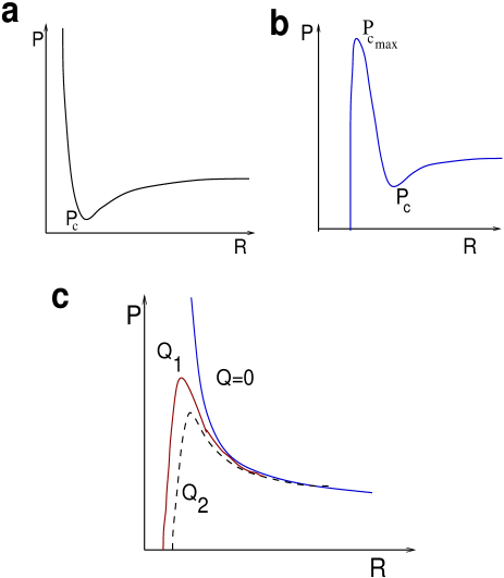
Figure 3: Illustration of the behavior of eqn.(9): $P$ shown as a function of $R$ for (top left) without charge and (top right) with charge. The introduction of charge changes the plot dramatically. The effect of charge $Q$ on a bubble is shown schematically for different values of $Q$, $Q_{2}>Q_{1}$, in the bottom figure. Note that our study in this paper is confined only to applied pressures in the range $0.4\times 10^{5}-1.5\times 10^{5}$ Pa.

To obtain the Blake radius for the charged bubble, we adapt the procedure for the uncharged case (see for example Harkin et al harkin ) to our situation. We first minimize equation (9) with respect to $R$, $R>0$. This leads to the quartic equation:

$$R^{4}-\frac{Q^{2}}{4\pi\epsilon\sigma}R-\frac{5}{2\sigma}\phi=0,$$ (11)

The Blake radius $R_{crit}$ is given by the real and positive root of this equation. We find that:

$$R_{crit} = \frac{1}{2\sqrt[6]{18a}}\Bigg{\{}\sqrt{\sqrt[3]{a^{2}}-\frac{10\sqrt[3]{12}\phi}{\sigma}}$$ (12)

$$+ \frac{\frac{6Q^{2}}{4\pi\epsilon\sigma}\sqrt{2a}-\Big{(}\sqrt[3]{a^{2}}-\frac{10\sqrt[3]{12}}{\sigma}\phi\Big{)}^{3/2}}{\left(\sqrt[3]{a^{2}}-\frac{10\sqrt[3]{12}}{\sigma}\phi\right)^{1/4}}\Bigg{\}}^{1/2}$$

where

$$a=\frac{9Q^{4}}{(4\pi\epsilon\sigma)^{2}}+\sqrt{3}\Big{(}\frac{27Q^{8}}{(4\pi\epsilon\sigma)^{4}}+\frac{4000}{\sigma^{3}}\phi^{3}\Big{)}^{1/2}.$$ (13)

The liquid pressure $p_{L_{crit}}$ corresponding to this critical value of the radius is obtained by substituting eqn.(9) back into eqn(4) :

$$p_{L_{crit}}=P_{v}+\frac{\phi}{R_{crit}^{5}}-\frac{2\sigma}{R_{crit}}+\frac{Q^{2}}{8\pi\epsilon R_{crit}^{4}}$$ (14)

The Blake threshold pressure may be obtained from the standard definition harkin :

$$p_{Blake}=P_{0}-p_{L_{crit}}$$ (15)

A rough estimate of the Blake radius and threshold can be made for sub-micron sized bubbles for which the contributions from the static pressure is negligible in comparison with the charge - corrected terms. In this approximation, we find that

$$R_{crit}\approx\frac{1}{2}(1+\sqrt[3]{18})\left(\frac{Q^{2}}{4\pi\epsilon\sigma}\right)^{1/3}=1.81\left(\frac{Q^{2}}{4\pi\epsilon\sigma}\right)^{1/3}$$ (16)

Substituting this in eqn.(8) and using eqn.(9), we find the following approximate expression for the Blake threshold:

$$p_{Blake}=P_{0}+\frac{Q^{2}}{8\pi\epsilon R_{crit}^{4}}\left(\frac{R_{0}}{R_{crit}}-1\right)+\frac{2\sigma}{R_{crit}}$$ (17)

$$= P_{0}+\left(\frac{4\pi\epsilon\sigma^{4}}{Q^{2}}\right)^{\frac{1}{3}}\left(-6.95+4.416R_{0}\left(\frac{4\pi\epsilon\sigma}{Q^{2}}\right)^{\frac{1}{3}}\right)$$

IV Rayleigh collapse and the influence of driving pressure amplitude

After the bubble attains its maximum radius $R_{max}$, it proceeds to the main collapse. Its dynamics during this phase is described by the Rayleigh equation:

$$R\ddot{R}+\frac{3}{2}{\dot{R}}^{2}=0.$$ (18)

In considering cavitation in this limit, one is essentially considering collapse of a void, ignoring all terms such as viscosity, surface tension, etc. The solution for this is found to be

$$R(t)=R_{r}\left(\frac{t_{c}-t}{T}\right)^{2/5},$$ (19)

where at $t=t_{c}$, the bubble collapses to a point $R=0$. $R_{r}$ is a characteristic radius, and $T$ is the time period of oscillation of the bubble. It may be noted that the characteristic radius $R_{r}$ in this scaling law is different from that reported in hilgenfeldt where the polytropic constant was taken to be unity, corresponding to an isothermal process. Here we find an estimate for $R_{r}$ for $\Gamma=5/3$, using a similar energy argument as in hilgenfeldt . Converting the potential energy $E_{pot}$ of the bubble at $R_{max}$ to kinetic energy at $R_{0}$ we get

$$\dot{R}=-\left(\frac{2P_{0}}{\rho R_{0}^{3}}\right)^{1/2}\left(\frac{4\pi}{3}\right)^{\frac{\Gamma-1}{2}}R_{max}^{3\Gamma/2}$$ (20)

Using Eqn.(19) in (20) we obtain

$$R_{r}=\left(\frac{25T^{2}P_{0}}{2\rho}\left(\frac{4\pi}{3}\right)^{\Gamma-1}\right)^{1/5}R_{max}^{3\Gamma/5}$$ (21)

For $\Gamma=5/3$, we get

$$R_{r}=\left(\frac{25T^{2}P_{0}}{2\rho}(\frac{4\pi}{3})^{\frac{2}{3}}\right)^{\frac{1}{5}}R_{max}\approx 2.006\left(\frac{P_{0}T^{2}}{\rho}\right)^{\frac{1}{5}}R_{max}$$ (22)

The extremely simplified expression, Eqn.(22), is none the less useful for making some physically relevant approximations. This approximation would hold best during the bubble’s collapse to a minimum radius $R_{min}$. It would also be less inaccurate when the dimensions of the collapsing bubble are very small, that is, when $R_{min}$ is very small. This would tend to match more closely those cases where the charge on the bubble is high, so that the reduction in values of $R_{min}$ is correspondingly more. We can see that in the presence of a driving frequency $\omega$ for the system, $R(t)$ would show a frequency dependence $R(t)\sim\omega^{2/5}$ in the regime near bubble collapse, at higher driving pressure amplitudes, so that we have

$$R_{min}\sim a_{1}\omega^{2/5},$$ (23)

$a_{1}$ being a prefactor with appropriate dimensions.
At higher driving frequencies, the bubble typically has larger values for its minimal radius, there not being sufficient time for complete collapse to occur before the expanding regime sets in. Increasing the charge present on the bubble enables it to reach smaller dimensions.
The minimum radius scaled by the driving frequency, through $R_{min}/\omega^{2/5}$ is shown in the plot of Figure (4a). As expected from the discussion above, best agreement of Eqn.(23), as evidenced through a superposition of all the curves for different frequencies, is best seen at higher charge values and lower $R_{min}$ values.

It is to be expected however, that in reality a stable bubble can not carry an indefinite magnitude of charge $Q$. This can also be seen on plotting the minimum radius $R_{min}$ as a function of charge, where, for a given driving pressure, the minimum radius of the bubble for every driving frequency converges to one value of the charge. This, however, needs to be modified as a further physical constraint to the system exists in that bubble contraction can not also indiscriminately progress indefinitely. The smallest dimensions that the bubble can take, that is, the least value of the minimum radius $R_{min}$ reached during the bubble’s compressive regime, is bounded by the value of the van der Waals hard core radius $h$. The value of $h$ is determined by the gas enclosed within the bubble. For example, for argon, $h$ has the value $h=R_{0}/8.86$. For $R_{0}=5\mu m$, this equals a value of 0.564 $\mu m$.
$R_{min}$ with this constraint is shown in Figure (4b).
There is a maximal value for the charge a bubble can carry for attainment to $R_{min}=h$ to be possible. This limiting value of the charge we denote by $Q_{h}$. This is shown in Figure (4b), where the minimum radius of collapse, $R_{min}$, has been plotted as a function of charge $Q$, for a bubble of initial radius $R_{0}=5\mu m$, and pressure amplitude $P_{s}=1.35P_{0}$. The minimal bound of $R_{min}=h$ has been shown by a dotted line. The point of intersection of the curve for a particular driving frequency with this line gives the value of $Q_{h}$.

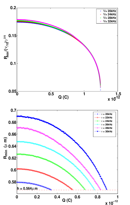
Figure 4: (a)(Above): $R_{min}$ scaled by $\omega^{2/5}$, plotted as a function of charge, $Q$, for various driving frequencies. (b)(Below): Minimum radius, $R_{min}$, plotted as a function of charge, $Q$, for various driving frequencies ($\nu=20,24,28,32$kHz); curves for higher frequencies are at the top. The horizontal dotted line corresponds to the cut-off $R_{min}=h$, the van der Waals hard core radius. $R_{0}=5\mu$m. (Color Online).

Correspondingly, there is an upper bound on the maximum radial velocity of the bubble $V_{max}$. The presence of charge on the bubble serves to reduce the effective magnitude of the surface tension. With increasing charge, the bubble is thus able to reach a smaller radius and a greater velocity. $V_{max}$ and $R_{max}$ as a function of charge $Q$ are shown in Fig.(5) for high driving pressure of $P_{s}=1.35P_{0}$. The limits to the curves in the plot are due to the limit in the maximal value $Q_{h}$ that $Q$ can take for each frequency.

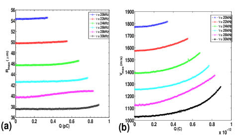
Figure 5: $R_{max}$ on the left, and $v_{max}$ on the right, plotted as a function of charge, $Q$, for various driving frequencies ($\nu=20,22,24,26,28,30$ kHz), lower frequency curves on the top. $R_{0}=5\mu$m, $P_{s}=1.35P_{0}$. (Color Online).

Furthermore, as the frequency of the driving ultrasonic acoustic wave is increased, the maximum radius attained by the bubble, $R_{max}$, reduces. This is understandable by recalling that the higher the frequency, the shorter is the period of negative pressure shear and the bubble is driven to cavitation collapse in a shorter time span resulting in shorter expansion time of the bubble. This also causes the value of the minimum radius to become larger with increasing frequency of the driving ultrasound wave. The larger the maximum radius reached, the more violent the collapse is, resulting in smaller minimum radius.

The system is very sensitive to changes in the pressure conditions. The amplitude $P_{s}$ of the driving pressure determines the physically viable minimal radius attainable by the bubble for a given charge. The maximal, bounding value of the charge, $Q_{h}$, reduces progressively with increasing amplitude of pressure $P_{s}$, until beyond a critical pressure $P_{m}$, it is no longer physically possible for the bubble radius to contract to such a small value. In Figure (6) we plot $Q_{h}$ as a function of $P_{s}$ for three different frequencies (20, 25 and 30 kHz). We show plots for two values of ambient bubble radius $R_{0}=2\mu m$ and $R_{0}=5\mu m$. Each curve demarcates two regions – the space below (or to the left of) the curve corresponds to the physically permissible region of $R_{min}>h$. The region above (or to the right of) each curve corresponds to $R_{min}<h$, which can not be reached in practice by a bubble of that corresponding ambient radius.

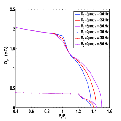
Figure 6: Plot of $Q_{h}$ as a function of driving pressure amplitude $P_{s}$, for bubbles of ambient radius $R_{0}=2\mu$m and $5\mu$m. The area below each curve corresponds to the domain where $R_{min}\geq h$. The region above each curve corresponds to $R_{min}<h$ and is physically unreachable for the bubble of that particular $R_{0}$. $R_{0}=5\mu$m, $\nu=20,25,30$kHz; $R_{0}=2\mu$m, $\nu=20,25,30$kHz. (Color Online).

It can be seen that the value of the critical pressure $P_{m}$ increases with driving frequency, and reduces with ambient radius $R_{0}$. At very low values of $P_{s}$, $Q_{h}$ becomes essentially independent of frequency for a given ambient radius. We denote the pressure where this frequency-independence first sets in (approached from above) by $P_{fi}$. It can be seen that $P_{fi}$ occurs at a lower value $P_{fi}=1.12P_{0}$ (with corresponding $Q_{h}\approx 1.3$ pC) for the larger bubble ($R_{0}=5\mu m$) than for the smaller bubble ($P_{fi}=1.2P_{0}$ for $R_{0}=2\mu$ m). Moreover there exists a brief crossover region for the $R_{0}=5\mu$ m bubble where the frequency-dependence of $Q_{h}$ reverses, before true frequency-independence of $Q_{h}$ occurs at ${P_{fi}}_{true}=0.9P_{0}$ (for $P_{s}>P_{fi}$, $Q_{h}$ for higher frequencies are greater than for lower values, while for ${P_{fi}}_{true}<P_{s}<P_{fi}$, this is reversed and $Q_{h}$ for higher frequencies are lower than that for lower frequencies for the $5\mu$m bubble).

To understand the effect of the driving pressure, we briefly paraphrase below the arguments given in hilgenfeldt for the isothermal case adapting it to our adiabatic system.

Combining the driving sound field with the static pressure plessetProsperetti the total external field $P_{ext}$ can be expressed as

$$P_{ext}=P_{0}(1-\alpha\cos\omega t).$$ (24)

Substituting this in the Rayleigh Plesset equation under quasistatic conditions:

$$\bigg{(}P_{0} - P_{v}+\frac{2\sigma}{R_{0}}-\frac{Q^{2}}{8\pi\epsilon R_{0}^{4}}\bigg{)}\bigg{(}\frac{R_{0}}{R}\bigg{)}^{3\Gamma}+\frac{Q^{2}}{8\pi\epsilon R^{4}}$$ (25)

$$- \frac{2\sigma}{R}-P_{0}(1-\alpha\cos\omega t)=0$$

we obtain the quintic equation

$$R^{5} - \frac{2\sigma}{(\alpha-1)P_{0}}R^{4}+\frac{Q^{2}}{8\pi\epsilon(\alpha-1)P_{0}}R$$ (26)

$$+ \frac{R_{0}^{5}}{\alpha-1}\left(1+\frac{2\sigma}{R_{0}P_{0}}-\frac{Q^{2}}{8\pi\epsilon R_{0}^{4}P_{0}}\right)=0$$

The behavior of the equation is completely determined by the quantity $\alpha-1$. For $P_{ext}>0$, we have a a stable, single solution for $R$. For negative, small amplitude $P_{ext}$ there are two solutions with that at lower $R$ being the stable one.
These two merge only at a critical value $P_{ext}=P_{Blake}$, $P_{Blake}<0$. For this, $P_{gas}>P_{ext}+P_{\sigma}$ is always the case and leaves the equation without a solution, where $P_{gas}=\phi/R^{5}$ and $P_{\sigma}=2\sigma/R$.

Liquid pressure becoming negative, opposes the confinement effect of the surface-tension contribution, $P_{\sigma}$. Once the bubble is larger than a critical radius $R_{c}$, pressure balance at the bubble wall can not be maintained, and explosive growth sets in. The bubble is unstable at this stage, and further growth leads to increased instability and still more expansion, and quasistatic conditions no longer hold.

With the time period of oscillation $T=2\pi/\omega$ being larger than the time scale of the bubble’s oscillations, oscillations of the external pressure can be considered as being quasistatic. For crossing the Blake threshold $P_{ext}<0$ is required so that $\alpha>1$. $t=0$ gives $P_{ext}=(\alpha-1)P_{0}$ to be negative. Thus the behavior shown by bubbles for $\alpha<1$ will be very different from that for $\alpha>1$; for values of $\alpha$ less than 1, bubble oscillations will tend to be less violently expansive and the effect of surface tension dominate the dynamics.

V Expansion - compression ratio and the transient threshold

The surface tension greatly influences bubble dynamics and can give rise to very distinct behaviours for bubbles of different ambient radii $R_{0}$, even when all other conditions are identical. In smaller bubbles, surface tension is a very dominant term. Looking at the $R_{min}$ vs. $P_{s}$ plots (Figure (7)) for $R_{0}=2\mu$m and $R_{0}=5\mu$m, we at once see a striking difference between the two. For the larger, 5 micron bubble, we see that on lowering the pressure $P_{s}$, at a value corresponding to $P_{s}=P_{fi}=1.12P_{0}$, the $R_{min}$ curves all converge to a point. Lowering $P_{s}$ further brings the bubble to a cross-over regime, until reaching a lower pressure $P_{s}={P_{fi}}_{true}\approx 0.9P_{0}$, below which pressure, the curves largely show frequency - and charge-independent behavior. As will be seen in the ensuing paragraphs, $P_{s}=P_{fi}$ is actually the transition pressure $P_{tr}$ beyond which violent bubble collapse occurs.

For the smaller, 2 micron bubble, we do not see any cross-over regime, and the pressure $P_{s}=P_{fi}=1.2P_{0}$ where all curves converge such that for $P_{s}<P_{fi}$ charge or frequency-dependence of the curves is suppressed, is actually less than the transition pressure $P_{tr}=1.3P_{0}$ for $R_{0}=2\mu$m.

Introduction of charge on the bubble serves to dramatically move $P_{tr}$ to a lower value, with the effective surface tension being reduced due to electrostatic interaction, and its effect being enhanced due to the bubble’s smaller dimensions.

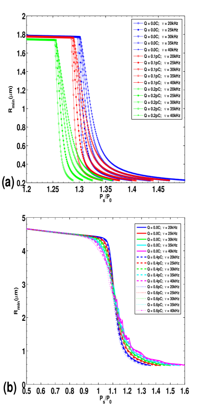
Figure 7: $R_{min}$ vs $P_{s}$ for different values of $\omega$ ($\nu=20,25,30,35,40kHz$) and $Q$. $Q=0C,0.1pC,0.2pC$ for (a) $R_{0}=2\mu$m and (b) $Q=0C,0.4pC,0.6pC$ for $R_{0}=5\mu$m. (Color Online).

One obvious measure of the relative extremal values of the bubble dimensions is $R_{max}/R_{min}$. Other measures used to quantify the bubble’s dimensions are the expansion ratio $E\equiv R_{max}/R_{0}$, and the compression ratio $C\equiv R_{min}/R_{0}$.

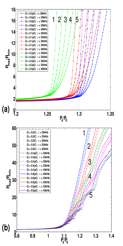
Figure 8: $R_{max}/R_{min}$ vs $P_{s}$ for different values of $\omega$ and $Q$, for a) $R_{0}=2\mu$m ($Q=0pC,0.1pC,0.2pC$); and b) $R_{0}=5\mu$m ($Q=0pC,0.4pC,0.6pC$) ($\nu=20,25,30,35,40kHz$). Curves labelled as 1,2,3,4, & 5 correspond to $\nu=20,25,30,35,40kHz$, respectively. Increasing $Q$ shifts curves upwards & to the left. (Color Online).

Figure (8) shows plots of the relative extremal bubble radius measure, $R_{max}/R_{min}$ as a function of the amplitude $P_{s}$ of the driving pressure wave for two different bubble radii: $R_{0}=2\mu$ m and $R_{0}=5\mu$ m. We introduce yet another useful and significant measure of the relative extent of bubble expansion to compression, which we term the expansion-compression ratio, $\zeta$

$$\zeta\equiv(E-1)/(1-C)=(R_{max}-R_{0})/(R_{0}-R_{min}).$$ (27)

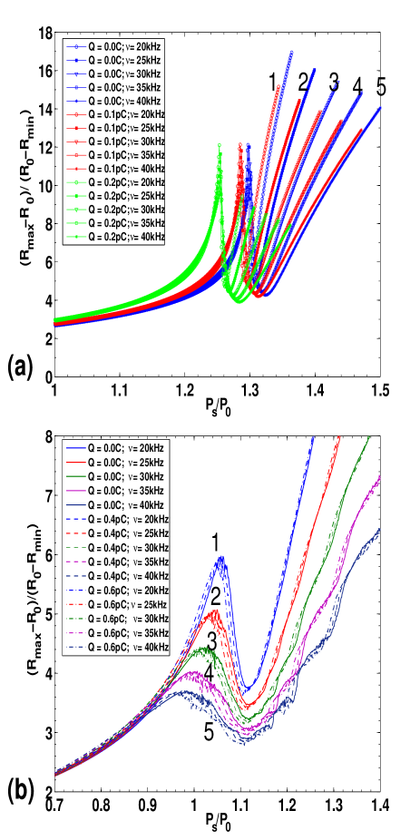
Figure 9: Expansion-Contraction ratio $\zeta$ for (a) $R_{0}=2\mu$m ($Q=0pC,0.1pC,0.2pC$) and (b) $R_{0}=5\mu$m ($Q=0pC,0.4pC,0.6pC$)as a function of $P_{s}$. Curves labelled as 1,2,3,4, & 5 correspond to $\nu=20,25,30,35,40kHz$, respectively. Increasing $Q$ shifts curves downwards & to the left. (Color Online).

Investigating the dependence of this EC ratio $\zeta$ on the amplitude of applied pressure $P_{s}$ yields some delightful results and clearly shows the great utility of this measure of bubble expansion/contraction. Figure (9) is a plot of $\zeta$ as a function of $P_{s}$ for two different ambient radius values, $R_{0}=2\mu$m and $R_{0}=5\mu$m. For bubbles with not too small ambient radius $R_{0}$ (for example, for $R_{0}=5\mu$m), at low values of $P_{s}$, the expansion-compression ratio $\zeta$ becomes independent of charge and frequency below some $P_{s}={P_{s}}_{l}$, and $\zeta$ curves for various frequencies and charges all superimpose (Figure(9(b))). This behaviour is not shown by smaller bubbles (for example, for $R_{0}=2\mu$m), whose $\zeta$ curves instead show distinct charge and frequency dependence even at very low amplitudes of driving pressure (Figure(9(a))).

In general for all bubble sizes, the following generic behaviour of the EC ratio $\zeta$ is shown: at lower pressures, till a certain pressure $P_{s}=P_{sl}$, $\zeta$ shows only very weak dependence on charge and driving frequency. In Figure (10(a)) the dashed and solid curves are shown as representative of different charge and frequency values, which are coincident at pressures below $P_{sl}$. With increasing $P_{s}$, the EC ratio increases to a peak at a critical pressure value $P_{b}$, followed by a short, steep dip upto a second critical pressure value $P_{tr}$. This is followed further by a regime of an ever-increasing $\zeta$ with increasing $P_{s}$ (Figure (10(a))). Between $P_{b}$ and $P_{tr}$ lies a region of negative slope, which is essentially an unstable, transient region.
Surface tension is overcome at a critical radius corresponding to the pressure $P_{b}$ after which significant bubble expansion occurs and the motion is transient until pressure $P_{tr}$. For $R_{0}$ being sufficiently large, bubble collapse can not be completed fully during the compression part of the cycle of applied pressure and bubble motion is then stable. This explanation accounts for the presence of two thresholds, enclosing a transient regime with stable regions on either side neppiras . At the lower threshold, it can be seen from Figures (9, 10) the transition from stable to transient conditions occurs very steeply.
The lower transient threshold pressure $P_{b}$ delineates a pressure value above which the bubble expansion occurs dramatically, and this in fact equals the Blake threshold pressure, $P_{b}=P_{Blake}$.

It is important to recall at this point that while the Blake threshold is a measure of the onset of rapid bubble expansion, it gives us no information at all about bubble implosion prosperettiUltra . The upper transient threshold pressure, $P_{tr}$, on the other hand, is the value of $P_{s}$ above which violent bubble contraction begins. It can be seen, by inspecting the $R_{min}$ versus $P_{s}$ curve (Figure 7) that at $P_{s}=P_{tr}$, $R_{min}=R_{0}/2$. This, in fact, identifies the transition to a strong collapse regime from weaker oscillations hilgenfeldt . This can be verified by incorporating the radial velocity into the EC plot. As can be seen in Figure (10(b)), where a scale representing the magnitude of maximum radial velocity has been included, it is only at driving pressures above the upper transient threshold $P_{tr}$ that velocities rise dramatically to high values, where as at lower $P_{s}$, the radial oscillations occur more slowly.

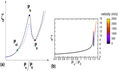
Figure 10: (a).The points on the graph where frequency & charge -independence sets in ($P_{sl}$), the Blake threshold ($P_{b}=P_{Blake}$) and the upper transient threshold pressure ($P_{tr}$) are shown in the schematic figure. The dashed and solid curves typify different charge and frequency values, which superimpose at pressures below $P_{sl}$. (b). Plot of the $\zeta$ curve with the key for the maximum radial velocity shown on the right, for a given frequency and charge. As can be seen, for pressures greater than the upper transient threshold pressure $P_{tr}$, bubble collapse occurs violently, at greater velocities. (Color Online).

In Figure (11)(a) and (b) we show the frequency response diagrams for the minimum radius and maximum velocity attained by a 5 micron bubble in water at the low driving pressure of $0.4P_{0}$ and carrying charges $Q=0,0.4,1.0$ and $1.24$pC. It is clear that increasing the magnitude of charge present on the bubble increases the magnitude of the response and advances it to lower frequencies. The peaks in the response diagram appear much earlier, at lower frequencies, for higher charges and their enhanced magnitudes (smaller minimum radius and larger maximal velocity) point to more violent collapse.

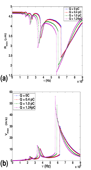
Figure 11: Frequency response curves for minimum radius (a) and maximum velocity (b) of the bubble. $R_{0}=5\mu$m, $Q=0pC,0.4pC,1.0pC,1.24pC$. (Color Online).

We can make a further, very rough estimate of the maximal bubble expansion limits at this transient pressure. We first consider the following vastly simplifying assumptions: that at $R\rightarrow R_{min}$, ${\dot{R}}\rightarrow c$, where $c$ is the speed of sound in the liquid. We further assume, for purpose of this estimation, that as $R\rightarrow R_{max}$, ${\dot{R}}\rightarrow 0$.
At its local minimum at $P_{s}=P_{tr}$, $\zeta=\zeta^{tr}$ will satisfy $({\frac{\partial\zeta}{\partial P_{s}}})|_{P_{s}=P_{tr}}=0$, so that we get

$$\frac{\partial R_{max}}{\partial P_{s}}=-\frac{R_{max}-R_{0}}{R_{0}-R_{min}}\frac{\partial R_{min}}{\partial P_{s}}=-\zeta^{tr}\frac{\partial R_{min}}{\partial P_{s}}.$$ (28)

Now using

$$\frac{\partial R_{min}}{\partial P_{s}} \approx \bigg{(}-5(P_{a}+\frac{2\sigma}{R_{0}}-\frac{Q^{2}}{8\pi\epsilon R_{0}^{4}})\frac{R_{0}^{5}}{R_{min}^{6}}+\frac{2\sigma}{R_{min}^{2}}$$

$$- \frac{4Q^{2}}{8\pi\epsilon R_{min}^{5}}+4\eta\frac{c}{R_{min}^{2}}\bigg{)}^{-1}$$

$$\frac{\partial R_{max}}{\partial P_{s}} \approx \bigg{(}-5(P_{a}+\frac{2\sigma}{R_{0}}-\frac{Q^{2}}{8\pi\epsilon R_{0}^{4}})\frac{R_{0}^{5}}{R_{max}^{6}}+\frac{2\sigma}{R_{max}^{2}}$$ (29)

$$- \frac{4Q^{2}}{8\pi\epsilon R_{max}^{5}}\bigg{)}^{-1},$$

in Equation (28), we get

$$\zeta^{tr} = -\left(\frac{5\phi}{R_{max}^{6}}-\frac{2\sigma}{R_{max}^{2}}+\frac{4Q^{2}}{8\pi\epsilon R_{max}^{5}}\right)\Big{/}$$ (30)

$$\left(\frac{5\phi}{R_{min}^{6}}-\frac{2\sigma}{R_{min}^{2}}+\frac{4Q^{2}}{8\pi\epsilon R_{min}^{5}}-\frac{4\eta c}{R_{min}^{2}}\right),$$

where $\phi/R_{0}^{5}$ denotes the equilibrium pressure of the gas in the bubble (Eqn.(6)).

If we further consider the extremal case of $R_{min}\approx h$, this becomes

$$\zeta^{tr}=-\frac{\left(\frac{5\phi}{R_{max}^{6}}-\frac{2\sigma}{R_{max}^{2}}+\frac{4Q^{2}}{8\pi\epsilon R_{max}^{5}}\right)}{\left(\frac{5\phi}{h^{6}}-\frac{2\sigma}{h^{2}}+\frac{4Q^{2}}{8\pi\epsilon h^{5}}-\frac{4\eta c}{h^{2}}\right)}.$$ (31)

Now extremizing equation (31) with respect to $R_{max}$ yields a quartic equation for $R_{max}=R_{max}^{tr}$ at $P_{s}=P_{tr}$

$$R_{max}^{4}-\frac{5Q^{2}}{8\pi\epsilon\sigma}R_{max}-\frac{15\phi}{2\sigma}=0.$$ (32)

In the uncharged case, $Q=0$, this simplifies to

$$R_{max}^{tr}=\left(\frac{15\phi}{2\sigma}\right)^{1/4},$$ (33)

which is the value of $R_{max}$ at the transition point at $P_{s}=P_{tr}$, made under all the simplifying assumptions mentioned above. It will be noted that for mid-sized microbubbles, for example for $R_{0}=5\mu$m (plots for which have been shown), the point of transition $P_{tr}$ is approximately a constant and is largely independent of the driving frequency or the charge.

A comparison of the estimate of $R_{max}$ so obtained from the above equation for the uncharged case to the value obtained numerically is given in Table 1 below. Though the estimated values are far from accurate in many cases, they do, nonetheless, give a quick and useful estimation of $R_{max}$ at a driving pressure equalling the upper transient threshold of pressure $P_{tr}$.

Table 1: $R_{max}^{tr}$ obtained from Eqn.(32) & graphically.

Table 1
$R_{0}$	$R_{max}^{tr}$ (eqn.)	$R_{max}^{tr}$ (graph)
2 $\mu$m	4.87 $\mu$m	7.14 $\mu$m
3 $\mu$m	7.78 $\mu$m	10.65 $\mu$m
4 $\mu$m	10.92 $\mu$m	12.64 $\mu$m
5 $\mu$m	14.23 $\mu$m	14.3 $\mu$m
7 $\mu$m	21.3 $\mu$m	17.1 $\mu$m

These estimates though rather crude, might provide useful measures for avoiding undesirable regimes involving violent bubble collapses in medical diagnostics and applications.

VI Conclusions

In this work we have investigated the dynamics of a bubble forced by an ultrasound field, and seen how charge influences its behaviour. Our calculations are for a system where an adiabatic equation of state prevails, with $\Gamma=5/3$. We make several interesting observations. Charge serves to reduce the effective surface tension of the bubble. This causes a charged bubble to not only expand to a larger radius as compared to a neutral bubble but also collapse to a smaller minimum radius, the lower bound of which is given by the van der Waals hard core radius. The charged bubble’s collapse is also more violent, with radial velocities being reached being greater. Charge influences and modifies the liquid pressure profile. The effects are more marked for bubbles of smaller dimensions, where surface tension has a predominant influence. Studies of the effect of the amplitude of the forcing pressure wave show that introduction of charge serves to lower the Blake threshold so that the transition to violent collapses and oscillations occur at lower levels of pressure, especially for microbubbles of smaller dimensions and submicron bubbles. We have obtained expressions for the Blake threshold in the presence of charge.

We introduce a measure of the extremal dimensions reached by a bubble, which is a quantity $\zeta=(E-1)/(1-C)$ where $E$ and $C$ are the expansion and compression ratios, respectively. The advantage of plotting $\zeta$ as a function of $P_{s}$ is that it captures the distinct positions and behaviors of both the Blake threshold pressure as well as the upper transient threshold pressure, between which points lies a regime of instability for the bubble.

The maximum magnitude of charge a bubble can carry in the system tends to converge to a single asymptotic value, $Q_{max}$, and likewise the minimum radius converges to a single value for all frequencies, which is however modulated by the radial length scale cut-off provided by the van der Waals hard core radius. Exceeding the magnitude of charge $Q_{h}$ causes the bubble to contract to values of $R_{min}$ that are less than $h$ which cannot be physically reached and hence provide a physical upper bound for the system’s charge. We also investigated Rayleigh collapse for the bubble, obtaining an expression for the characteristic Rayleigh radius $R_{r}$. Frequency-dependence of the minimum radius is also captured. We also obtain approximate relations for the maximal radius at the critical transition point. Most of the numerical results presented in this work are for high pressures, corresponding to regimes of violent bubble collapse. We have demonstrated the importance of including charge in investigating the expansion and contraction of a bubble under forcing. We have also found scaling relations for extremal radial dimensions. Other results, including an investigation of the bifurcation structure as a function of charge, scaling relations for the maximal charge, etc. are being reported elsewhere ashok .

References

- (1) Lord Rayleigh, “On the pressure developed in a liquid during the collapse of a spherical cavity”,Philos. Mag. 34, 94-98 (1917).
- (2) E. A. Neppiras, “Acoustic cavitation”, Phys. Rep. 61, 159-251 (1980).
- (3) M. Minnaert, “On musical air-bubbles and sounds of running water”, Philos. Mag. 16, 235-248 (1933).
- (4) M. Versluis, B. Schmitz, A. von der Heydt and D. Lohse, “How snapping shrimp snap: through cavitating bubbles”, Science 289, 2114-2117 (2000).
- (5) P. Marmottaant and S. Hilgenfeldt, “A bubble-driven microfluidic transport element in bioengineering”, Proc. Natl. Acad. Sci. U.S.A. 101, 9523-9527 (2004).
- (6) K. S. Suslick, “Sonochemistry”, Science 247, 1439-1445 (1990).
- (7) T. J. Mason, “Sonochemistry”, Oxford University Press, New York, 92 pages (1999).
- (8) H. Frenzel and H. Schultes, “Lumineszenz in ultraschall-beschickten Wasser”, Z. Phys. Chem. Abt. B 27B, 421 (1934).
- (9) D. F. Gaitan, “An experimental investigation of acoustic cavitation in gaseous liquids, Ph. D. thesis, The University of Mississippi”, (1990).
- (10) D. F. Gaitan, L. A. Crum, C. C. Church and R. A. Roy, “Sonoluminescence and bubble dynamics for a single stable cavitation bubble”, J. Acoust. Soc. Am. 91, 3166-3183 (1992).
- (11) D. F. Gaitan and G. Holt, “Nonlinear bubble dynamics and light emission in single bubble sonoluminescence”, J. Acoust. Soc. Am. 103, 3046 (1998).
- (12) B. P. Barber and S. J. Putterman, “Observation of synchronous picosecond sonoluminescence”, Nature 352, 318-320 (1991).
- (13) M. P. Brenner, S. Hilgenfeldt and D. Lohse, “Single-bubble sonoluminescence”, Rev. Mod. Phys. 74, 425-484 (2002).
- (14) W. Lauterborn and E. Suchla, “Bifurcation superstructure in a model of acoustic turbulence”, Phys. Rev. Lett. 53, 2304-2307 (1984).
- (15) P. Smereka, B. Birnir and S. Banerjee, “Regular and chaotic bubble oscillations in periodically driven pressure fields”, Phys. Fluids 30, 3342-3350 (1987).
- (16) W. Lauterborn and U. Parlitz, “Methods of chaos physics and their applications to acoustics”, J. Acoust. Soc. Am. 84, 1975-1993 (1988).
- (17) U. Parlitz, V. Englisch, C. Scheffczyk and W. Lauterborn, “Bifurcation structure of bubble oscillators”, J. Acoust. Soc. Am. 88, 1061-1077 (1990).
- (18) C. E. Brennen, “Cavitation and Bubble Dynamics”, Oxford University Press, New York, 282 pages (1995).
- (19) H. A. McTaggart, “The electrification at liquid-gas surfaces”, Phil. Mag. 27, 297-314 (1914).
- (20) T. Alty, “The cataphoresis of gas bubbles in water”, Proc. Roy. Soc. (London) 106, 315-320 (1924).
- (21) T. Alty, “The origin of the electric charge on small particles in water”, Proc. Roy. Soc. (London) A 112, 235-251 (1926).
- (22) V. A. Akulichev, “Hydration of ions and the cavitation resistance of water”, Sov. Phys. Acoust. 12, 144-149 (1966).
- (23) M. B. Shiran and D. J. Watmough, “An investigation on the net charge on gas bubble induced by 0.75MHz under standing wave condition”, Iranian Phys. J. 2, 19-25 (2008).
- (24) M. Plesset, “The dynamics of cavitation bubbles”, J. Appl. Mech. 16, 277-282 (1949).
- (25) M. Plesset, “On the stability of fluid flows with spherical symmetry”, J. Appl. Mech. 25, 96-98 (1954).
- (26) B. E. Noltingk and E. A. Neppiras, “Cavitation produced by ultrasonics”, Proc. Phys. Soc. London Sec. B 63, 674-685 (1950).
- (27) J. B. Keller and I. I. Kolodner, “Damping of underwater bubble oscillations”, J. Appl. Phys. 27, 1152-1161 (1956).
- (28) J. B. Keller and M. Miksis, “Bubble oscillations of large amplitude”, J. Acoust. Soc. Am. 68, 628-633 (1980).
- (29) M. Plesset and A. Prosperetti, “Bubble dynamics and cavitation”, Ann. Rev. Fluid Mech. 9, 145-185 (1977).
- (30) A. Prosperetti, L. A. Crum and K. W. Commander, “Nonlinear bubble dynamics”, J. Acoust. Soc. Am. 83, 502-514 (1988).
- (31) N. F. Bunkin and F. V. Bunkin, “Bubbstons: stable microscopic gas bubbles in very dilute electrolytic solutions”, Sov. Phys. JETP. 74, 271-278 (1992).
- (32) A. I. Grigor’ev and A. N. Zharov, “Stability of the equilibrium states of a charged bubble in a dielectric fluid”, Technical Physics 45, 389-395 (2000).
- (33) Anthony A. Atchley, “The Blake threshold of a cavitation nucleus having a radius-dependent surface tension”, J. Acoust. Soc. Am. 85, 152-157 (1989).
- (34) T. Hongray, B. Ashok and J. Balakrishnan, “Oscillatory dynamics of a charged microbubble under ultrasound”, submitted, (2013).
- (35) B. P. Barber, R. A. Hiller, R. Löfstedt, S. J. Putterman, and K. R. Weninger, “Defining the unknowns of sonoluminescence”, Phys. Rep. 281, 65-143 (1997).
- (36) R. E. Apfel, “Acoustic cavitation prediction”, J. Acoust. Soc. Am. 69, 1624-1631 (1981).
- (37) A. Harkin, A. Nadim and T. J. Kaper, “On acoustic cavitation of slightly subcritical bubbles”, Phys. Fluids 11, 274-287 (1999).
- (38) S. Hilgenfeldt, M. P. Brenner, S.Grossmann and D. Lohse, “Analysis of Rayleigh-Plesset dynamics for sonoluminescing bubbles”, J. Fluid Mech. 365, 171-204 (1998).
- (39) A. Prosperetti, “Bubble phenomena in sound fields: part one”, Ultrasonics 22, 69-77 (1984).