Star formation in the luminous YSO IRAS 18345-0641

Abstract

Aims. We aim to understand the star formation associated with the luminous young stellar object (YSO) IRAS 18345-0641 and to address the complications arising from unresolved multiplicity in interpreting the observations of massive star-forming regions.

Methods. New infrared imaging data at sub-arcsec spatial resolution are obtained for IRAS 18345-0641. The new data are used along with mid- and far-IR imaging data, and CO ($J=3-2$) spectral line maps downloaded from archives to identify the YSO and study the properties of the outflow. Available radiative-transfer models are used to analyze the spectral energy distribution (SED) of the YSO.

Results. Previous tentative detection of an outflow in the H₂ (1-0) S1 line (2.122 $\mu$m) is confirmed through new and deeper observations. The outflow appears to be associated with a YSO discovered at infrared wavelengths. At high angular resolution, we see that the YSO is probably a binary. The CO (3–2) lines also reveal a well defined outflow. Nevertheless, the direction of the outflow deduced from the H₂ image does not agree with that mapped in CO. In addition, the age of the YSO obtained from the SED analysis is far lower than the dynamical time of the outflow. We conclude that this is probably caused by the contributions from a companion. High-angular-resolution observations at mid-IR through mm wavelengths are required to properly understand the complex picture of the star formation happening in this system, and generally in massive star forming regions, which are located at large distances from us.

1 Introduction

It is now understood through recent studies that massive stars, at least up to late-O spectral types, form primarily through disk accretion and driving outflows (e.g. Arce et al. arce07 (2007), Beuther et al. 2002b , Davis et al. davis04 (2004), Varricatt et al. varricatt10 (2010)). However, they are known to form in clusters in giant molecular clouds that are located mostly along the galactic plane at large distances from us. The spatial resolution and wavelength coverage of most of the studies available are insufficient to probe their multiplicity, which often lead to inaccuracies in the estimates of the properties of the YSOs, their disks and outflows. Detailed studies of individual sources are therefore necessary, which were often not feasible in surveys though which they were identified. In this paper, we present the results of a multi-wavelength observational study of the luminous YSO IRAS 18345-0641 (hereafter IRAS 18345) and discuss the complications associated with treating a YSO as single, where it is possibly composed of two or more components.

IRAS 18345 was identified as a candidate ultra-compact Hii region by van der Walt, Gaylard & MacLeod (vanderwalt95 (1995)), who detected a 6.7 GHz methanol maser from its vicinity. Highly variable and multi-component 6.7 GHz Class-I methanol maser emission has been later detected towards this source by several other investigators (Szymczak, Hrynek & Kus szymczak02 (2000); Szymczak et al. szymczak02 (2000); Sridharan et al. sridharan02 (2002); Beuther et al. 2002c ; Pestalozzi, Minier & Booth pestalozzi05 (2005); Bartkiewicz et al. bartkiewicz09 (2009)). Bronfman, Nyman & May (bronfman96 (1996)) detected CS(2-1) emission from a dense core associated with IRAS 18345 at V_LSR=95.9 km s^-1. A distance of 9.5 kpc has been estimated with the distance ambiguity solved (Sridharan et al. sridharan02 (2002)).

H₂O maser emission is used as a tracer of the early stages of massive star formation, and is believed to be excited by jets (e.g. Felli, Palagi & Tofani felli92 (1992)). This source hosts H₂O maser emission (Sridharan et al. sridharan02 (2002); Beuther et al. 2002c ), showing its youth. OH maser emission (1612 MHz), which is known to be a tracer of circumstellar disks, has also been detected towards IRAS 18345 (Edris, Fuller & Cohen edris07 (2007); V_peak=93.52 km s^-1).

Beuther et al. (2002b ) mapped a massive molecular outflow from this source in the ¹²CO ($J=2-1$) line. The outflow was seen to be oriented NW-SE, with a projected length of 40″(1.84 pc) and a collimation factor f_c=1.5. C¹⁸O (2-1) observations by Thomas & Fuller (thomas08 (2008)) detected a line that was best fit by a narrow and a broad Gaussian component at 95.65 and 95.79 km s^-1 respectively indicating that they are likely to be associated with the same core or material; they suggest that the broad component is related to the outflow. Beuther et al. (2002a ) detected a possible outflow source at 1.2 mm (integrated flux density=1.4 Jy) using MAMBO array and the IRAM 30-m telescope. This source was also detected at 1.1 mm with an integrated flux of 0.92($\pm$0.12) Jy in the Bolocam Galactic Plane Survey conducted using the Caltech Submillimeter Observatory (Rosolowsky et al. rosolowsky10 (2010)), and at 450 and 850 $\mu$m in the survey of high-mass protostellar candidates using JCMT and SCUBA (Williams, Fuller & Sridharan williams04 (2004)).

Varricatt et al. (varricatt10 (2010)) imaged this region in the near-IR $K$ band and in a narrow-band filter centred at the wavelength of the H₂ (1-0) S1 line at 2.122 $\mu$m as a part of their imaging survey of massive YSOs. They had a tentative detection of an outflow as an H₂ line emission knot (MHO 2211; see Figure A20 of Varricatt et al). They detected two extremely red near-IR sources (labelled ‘A’ [$\alpha$ = 18:37:17.00, $\delta$ = -06:38:24.5] and ‘B’ [$\alpha$ = 18:37:16.91, $\delta$ = -06:38:30.7]). Source ‘B’ detected by them was very close to the IRAS source, the 1.2-mm continuum peak of Beuther et al. (2002a ) and the CH₃OH masers detected by Beuther et al. (2002c ).

IRAS 18345 is likely to be in a pre-UCHii phase. Radio emission is very weak towards this source. Hofner et al. (hofner11 (2011)) detected a faint (210 $\mu$Jy) unresolved 1.3-cm radio continuum source located at $\alpha$=18:37:16.91 $\delta$=-06:38:30.4. They propose that the radio emission was from an ionized jet driving the massive CO outflow detected by Beuther et al. (2002b ). (Sridharan et al. (sridharan02 (2002)) reported a 27-mJy 3.6-cm source towards IRAS 18345. However, Hofner et al. (hofner11 (2011)) pointed out that this emission was from an unrelated source located 3′SE of the IRAS source).

2 Observations and data reduction

2.1 UKIRT data

2.1.1 WFCAM near-IR data

We observed this region on multiple epochs using the United Kingdom Infrared Telescope (UKIRT), Hawaii, and the UKIRT Wide Field Camera (WFCAM; Casali et al. casali07 (2007)) during the UKIDSS backup time. Observations were performed using the near-IR J, H and K MKO consortium filters and a narrow band filter centered at the wavelength of the H₂ (1-0) S1 line at 2.1218 $\mu$m. WFCAM employs four 2048$\times$2048 HgCdTe HawaiiII-2RG arrays; for the observations presented here, we used the data from only one of the four arrays in which the object was located. At a pixel scale of 0.4″ pixel^-1, each array has a field of view of 13.5′$\times$13.5′. Observations were carried out by dithering the object to 9 positions separated by a few arcseconds in J, H and K bands, and to 5 positions in H₂, and using a 2$\times$2 microstep, resulting in a pixel scale of 0.2″ pixel^-1. Table 1 gives a log of the WFCAM observations performed.

Table 1: Log of WFCAM observations

UTDate	Filters	Exp.	Total int.	FWHM
(yyyymmdd)	used	time (s)	time (s)	(arcsec)
20120401	$K$	5,1	180,72	0.82,0.84
20120407	$J,H$	10,5	180,360	1.11,0.99
20120426	$J$	10	360	0.66
20120501	$H_{2}$	40	800,800	0.95,0.83
20120522	$H_{2},K,K$	40,5,1	800,180,72	1.26,1.18,1.16

The data reduction, and archival and distribution were carried out by the Cambridge Astronomical Survey Unit (CASU) and the Wide Field Astronomy Unit (WFAU) respectively. Since the photometric calibrations are performed using point sources present in all dithered frames and using their 2MASS magnitudes, the photometric quality is good even in the presence of clouds. The photometric system and calibration are described in Hewett et al. (hewett06 (2006)) and Hodgkin et al. (hodgkin09 (2009)) respectively. The pipeline processing and science archive are described in Irwin et al. (irwin04 (2004)) and Hambly et al (hambly08 (2008)). The left panel of Figure 1 shows a JHK colour composite image created from the WFCAM data in a 1.5$\arcmin\times$1.5$\arcmin$ field centred on IRAS 18345. Sources ‘A’ and ‘B’ are labelled on the figure. Both sources are detected in K. This region was also observed in the $JHK$ bands using WFCAM as a part of the UKIRT Infrared Deep Sky Survey (UKIDSS; Lawrence et al. lawrence07 (2007)). We downloaded the JHK images (obtained for the Galactic Plane Survey, GPS) and merged catalogs from the UKIDSS GPS DR6+.

Source ‘A’ is saturated in our images with 5 sec exposure, so its K magnitude is derived from a mosaic obtained with per frame exposure time of 1 sec on 20120522 UT. It is detected well in H band. We detect a very faint source at the location of ‘A’ in the $J$ band image obtained on 20120426 UT, when the seeing was good. It has a faint neighbour $\sim$0.8″NE. Hence its magnitudes are measured using an aperture of radius 0.4″and applying aperture corrections. ‘B’ is detected well in $K$ as a point source embedded in nebulosity. Its estimated magnitudes are affected by the presence of nebulosity, with the K-magnitudes in a 3″-diameter aperture brighter than that in a 2″-diameter aperture by  0.21 mag. ‘B’ is not detected in J and only the nebulosity associated with it is detected in H. Table 2 shows the magnitudes of the two sources measured on different epochs.

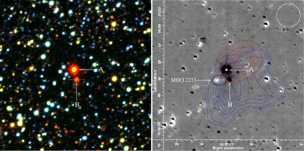
Figure 1: The left panel shows WFCAM $JHK$ colour-composite image ($J$-blue, $H$-green, $K$-red), and the right panel shows the continuum-subtracted H₂ image, smoothed with a Gaussian of FWHM=2 pix, and averaged over all our observations. The images are constructed from our new WFCAM data, and cover a filed of view of 1.5′$\times$1.5′. The dashed yellow line on the $JHK$ image shows the location and direction of the major axis (length $\times$50) of the elliptical distribution of the 6.7 GHz methanol maser spots detected by Bartkiewicz et al. (bartkiewicz09 (2009)). The blue (continuous) and red (dashed) contours overlaid on the H₂ image show the deconvolved blue- and red-shifted lobes of the outflow detected in CO (J=3-2) (see §2.3.1); the blue contours are at 3, 5, 10, 15, 20, 25, 30 and 40 $\sigma$, and the red contours are at 3, 5, 7, 9, and 11 $\sigma$ above the mean background. The H₂ line emission features are enclosed in ellipse and labelled “MHO 2211”. The white circle on the top-right corner shows the JCMT beam size (14.6″at 345 GHz).

The H₂ images were continuum subtracted using scaled $K$ band images. The background emission was fitted and removed from the H₂ and $K$ band mosaics. The seeing obtained in our K band mosaics was better than in H₂. For any H₂ mosaic, the K band mosaic with the closest seeing was used for continuum subtraction, after smoothing the K band mosaic with a suitable Gaussian to match FWHM in the H₂ mosaic. The average of the ratio of counts K/H₂ was evaluated for a few isolated point sources present in both K and H₂ mosaics. The background-subtracted $K$ mosaics were scaled by these ratios and were subtracted from the background-subtracted H₂ mosaics to perform the continuum subtraction. The three H₂ mosaics were continuum subtracted, smoothed with a Gaussian of FWHM=2 pixels to enhance the appearance of the faint line emission features and averaged. The right panel of Figure 1 shows the continuum-subtracted H₂ image of the same region as in the JHK colour composite in the left.

Table 2: Near-IR magnitudes of sources ‘A and ‘B’. A blank space is given when the observations were not done in a particular filter on any given UTDate.

UTdate	Magnitudesa
YYYYmmdd	$J$	$H$	$K$
Source ‘A’; $\alpha$=18:37:17.016, $\delta$=-6:38:24.36
20070826b	not resolved	12.82 (0.01)	Saturated
20120407	not detected	12.81 (0.01)
20120426	20.14 (0.15)
20120522			8.82 (0.01)
Source ‘B’; $\alpha$=18:37:16.896, $\delta$=-6:38:30.48
20031009c			12.69 (0.01)
20070826b		15.934 (0.016)	12.45 (0.01)
20120401			12.82 (0.01)
20120407	not detected	16.17 (0.05)
20120522	not detected		12.53 (0.01)

• are in the UKIRT photometric system, measured using an aperture of diameter 2″and applying aperture corrections. The values given in parenthesis are the 1-$\sigma$ internal errors. ^bFrom UKIDSS GPS DR6+. ^cFrom the images presented in Varricatt et al. (varricatt10 (2010)) observed using UKIRT and UFTI; the data of all other nights were obtained using UKIRT and WFCAM.

2.1.2 IRCAM3 imaging in $L^{\prime}$ and $M^{\prime}$ bands

$L^{\prime}$ and $M^{\prime}$ imaging observations of IRAS 18345 were performed using UKIRT and the facility 1–5-$\mu$m imager IRCAM3. IRCAM3 uses a 256 $\times$ 256 InSb array and gives a total field of view of 20.8″$\times$20.8″with an image scale of 0.081″ pix^-1 at the Cassegrain focal plane of UKIRT. The $L^{\prime}$ and $M^{\prime}$ observations were performed on 20000715 and 20000716 UT respectively. Individual exposure times of 0.2 sec and 0.12 sec with 100 coadds were used in $L^{\prime}$ and $M^{\prime}$ respectively. Observations were performed by offsetting the field to 4 positions on the array, separated by 15″each in RA and Dec. This 4-point jitter pattern was repeated thrice. The adjacent frames were subtracted from each other and are flat fielded. This resulted in a mosaic with two positive and two negative beams for the target. Two of the four offset positions were outside the array and in one of the remaining two, source ‘A’ was outside the array; hence, the total exposure time for ‘A’ and ‘B’ were 60 and 120 sec respectively in $L^{\prime}$ and 36 and 72 sec respectively in $M^{\prime}$.

The sky conditions were photometric on both nights. The excellent seeing on 20000716 ($\sim$0.34″) during the $M^{\prime}$ observations enabled us to resolve source ‘B’ into two components ‘B1’ and ‘B2’ for the first time. These two components are at a separation of $\sim$0.45″in the SE-NW direction, with ‘B1’ located SE of ‘B2’. Figure 2 shows the $M^{\prime}$ image of the central region of IRAS 18345 with the sources ‘A’ and ‘B’ detected. The contours generated from the $K$-band image are overlaid on Figure 2. The insets on the right show a 1.5″ $\times$ 1.5″field containing source ‘B’ in $M^{\prime}$. ‘B1’ and ‘B2’ are labelled on the figure.

When compared with that in $M^{\prime}$, the seeing was poor and variable during the $L^{\prime}$ observations (FWHM$\sim$0.61″in the mosaic), hence ‘B’ is not resolved in the final mosaic in $L^{\prime}$. However, the seeing was better (FWHM$\sim$0.38″) for two offset positions (40-s exposure) of the $L^{\prime}$ observations; an $L^{\prime}$ mosaic in a 1.5″$\times$1.5″field around ‘B’ constructed using those two frames is shown in the bottom-left inset in Figure 2. Photometric standards were observed in $L^{\prime}$ and $M^{\prime}$ for flux calibration. The magnitudes were derived using an aperture of diameter 4.07″(50 pixels) and applying extinction corrections for the differences in the airmass between the object and the standard stars. The $M^{\prime}$-band photometry of ‘B1’ and ‘B2’ were derived using a 0.326″(4 pixels)-diameter aperture and applying aperture corrections (derived from source ‘A’ in the $M^{\prime}$-band mosaic, and from standard stars for the $L^{\prime}$ frames). Source ‘B’ detected in our $K$-band image is centred on ‘B1’, with a nebulous extension in the direction of ‘B2’. Astrometric calibration of the $L^{\prime}$ and $M^{\prime}$ images were performed using the coordinates of ‘A’ and ‘B1’ measured from the $K$-band image. The coordinates and magnitudes of the sources detected are given in Table 3.

Table 3: IRCAM3 imaging in $L^{\prime}$ and $M^{\prime}$ bands and Michelle imaging at 12.5 $\mu$m

Source	RAa	Deca	IRCAM3 magnitudesb		Michelle flux (Jy)b
identification			$L^{\prime}$	$M^{\prime}$	12.5 $\mu$m
A	18:37:17.005	-06:38:24.5	5.15 (0.01)	4.59 (0.04)	4.53 (0.18)
B1+B2			8.53 (0.02)	6.71 (0.05)	1.56 (0.10)
B1	18:37:16.917	-06:38:30.77	9.65 (0.09)	7.21 (0.06)
B2	18:37:16.897	-06:38:30.43	10.12 (0.09)	7.98 (0.06)

• ^aFrom the IRCAM images. ^aThe values given in parenthesis are the 1-$\sigma$ errors - in the zero points for IRCAM3, and in the flux measured in the 4 beams for MICHELLE.

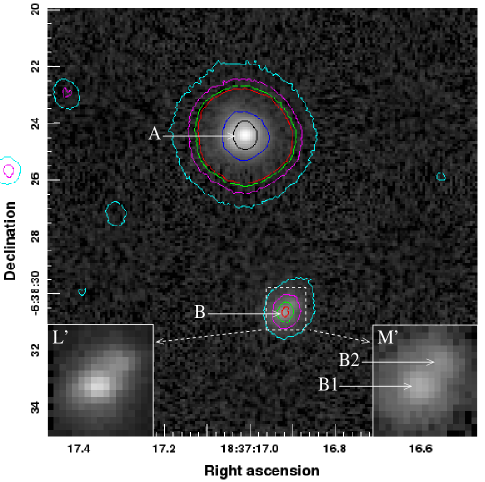
Figure 2: $M^{\prime}$-band image of the central 15″$\times$15″field around IRAS 18345 Contours from the UFTI $K$-band image of Varricatt et al. (varricatt10 (2010)) are overlaid. The bottom-left and bottom-right insets show 1.5″$\times$1.5″fields surrounding source ‘B’ in $L^{\prime}$ and $M^{\prime}$ respectively.

2.1.3 Michelle imaging at 12.5 $\mu$m

We observed IRAS 18345 using using UKIRT and Michelle on 20040329 UT. Michelle (Glasse et al. glasse97 (1997)) is a mid-infrared imager/spectrometer using an SBRC Si:As 320x240-pixel array and operating in the 8–25 $\mu$m wavelength regime. It has a field of view of 67.2″$\times$50.4″with an image scale of 0.21″/pix at the Cassegrain focal plain of UKIRT.

The Michelle observations were obtained using a filter centered at 12.5 $\mu$m with 9% passband. The sky conditions were photometric. BS 6705 and BS 7525 were used as standard stars. The observations were performed by chopping the secondary in the N-S direction and nodding the telescope in the E-W by 15″each (peak-peak) to detect faint sources in the the presence of strong background emission. Data reduction was performed using the UKIRT pipeline orac-dr (Cavanagh et al. cavanagh08 (2008)) and Starlink kappa (Currie et al. currie08 (2008)). The resulting mosaic has four images of the sources detected (2 positive and 2 negative beams). The final image was constructed after negating the negative beams and combining all four beams. Figure 3 shows a 15″$\times$15″field of the mosaic surrounding IRAS 18345. An average FWHM of 0.98″was measured from the sources detected in the 12.5 $\mu$m image. The astrometric corrections were applied by adopting the position of source ‘A’ from Varricatt et al. (varricatt10 (2010)). The coordinates derived for the fainter 12.5-$\mu$m source agrees well with that of the near-IR source ‘B’ detected by Varricatt et al. (varricatt10 (2010)). The fluxes measured for ‘A’ and ‘B’ are given in Table 3. At this spatial resolution, the two components of ‘B’ are not resolved.

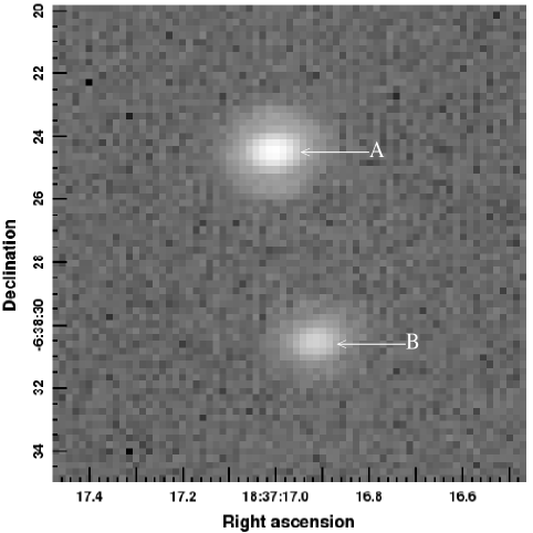
Figure 3: Michelle 12.5-$\mu$m image of IRAS 18345 covering a field of 15″$\times$15″.

2.2 Methanol observations

The $J$=5–4 (241.80 GHz) and $J$=7–6 (338.53 GHz) transitions of methanol were observed using the 15-m James Clerk Maxwell Telescope (JCMT), Hawaii, in July and August 2004. The receiver RxA (211–279 GHz) was used for the $J=5-4$ transition and receiver RxB3 (315–373 GHz) was used for $J$=7–6. In both cases the back end was the DAS (Digital Autocorrelator Spectrometer) with a bandwidth and spectral resolution of 250 MHz and 0.16 MHz respectively for $J$=5–4, and 500 MHz and 0.625 MHz respectively for $J$=7–6. Pointing at the JCMT was checked every hour and had an rms $<$2.5^′′. The weather was good during the observations, with opacities in the range 0.13$<\tau_{225}<$0.16. The data were reduced using the data reduction package specx (Prestage et al. prestage00 (2000)). Figure 4 shows the methanol spectra.

CH₃OH, is an organic molecule that originates primarily on the surface of grains, usually seen towards hot cores. Organic molecules such as these appear in the gas phase once sufficient ices have been evaporated from the grain surfaces. This implies gas temperatures in excess of 100 K (Rodgers & Charnley rodgers03 (2003)). These conditions are achieved either through the localized heating of the region immediately surrounding the young star, or in the shocked regions produced by a powerful outflow.

Table 4 shows the rest frequencies, observed radial velocities, intensities and line widths of the prominent methanol lines detected in our spectra. The line identifications are adopted from Anderson, De Lucia & Herbst (anderson90 (1990)) and Maret et al. (maret05 (2005)). The lines are mostly centred at the $\upsilon$_LSR of the core, and have large width, suggesting that they originate in a warm region surrounding the core.

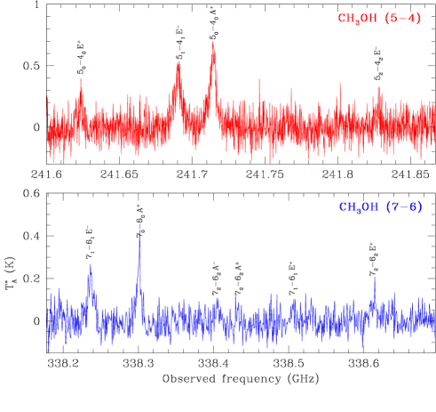
Figure 4: CH₃OH ($J$=7–6; 338.53 GHz) and ($J$=5–4; 241.80 GHz) spectra observed using JCMT.

Table 4: Methanol lines detected

Line ID	Rest Freq.	Eup	Radial	Width	Amp.	$\int$T${}_{A}^{*}$
	(GHz)	(K)	Vel.	(km/s)	T${}_{A}^{*}$(K)	(K km/s)
CH3OH (7–6)
71–61 E-	338.344605	69.61	95.4	7.25	0.16	1.21
70–60 A+	338.408718	64.98	95.4	5.33	0.28	1.60
72–62 E+	338.721694	86.31	95.5	9.22	0.06	0.61
CH3OH (5–4)
50–40 E+	241.700168	46.99	95.2	8.03	0.13	0.97
51–41 E-	241.767247	39.45	95.2	8.88	0.37	3.54
50–40 A+	241.791367	34.82	95.4	7.16	0.53	4.35
52–42 E-	241.904643	59.78	95.2	5.11	0.11	0.52

2.3 Archival data

IRAS18345 was detected well in the sky surveys conducted using the Wide-field Infrared Survey Explorer (WISE; Wright et al. wright10 (2010)) and the AKARI satellite (Murakami et al., murakami07 (2007)). The WISE mission surveyed the sky in four bands - $W$1 (3.4 $\mu$m), $W$2 (4.6 $\mu$m), $W$3 (12 $\mu$m) and $W$4 (22 $\mu$m). At the 6.1$\arcsec$–12.0$\arcsec$ spatial resolution of WISE, sources ‘A’ and ‘B’ are not resolved; however, the excellent positional accuracy (0.15$\arcsec$) of the WISE data enables the identification of the source. The location of the WISE source is in between ‘A’ and ‘B’; at the shorter wavelengths the centroid is closer to ‘A’, while at 22 $\mu$m, it is located very close to ‘B’ (see Figure 5) confirming that ‘B’ is the leading contributor at longer wavelengths. At the FWHM of $\sim$5.7″at 9 and 18 $\mu$m (Ishihara et al. ishihara10 (2010)), and 30–40″at 65, 90, 140 and 160 $\mu$m (Doi et al. doi09 (2009)) of the AKARI data, sources ‘A’ and ‘B’ are not resolved.

This region was observed in the Spitzer GLIMPSE II survey using the Infrared Array Camera (IRAC; Fazio et al. fazio04 (2004)) in bands 1–4, centered at 3.6, 4.5, 5.8 and 8.0 $\mu$m respectively. Spitzer also observed this region using the Multiband Imaging Photometer for Spitzer (MIPS; Rieke et al. rieke04 (2004)) at 24 $\mu$m and 71 $\mu$m. The reduced Spitzer images and point source photometry were downloaded from the NASA/IPAC Infrared Science Archive. Figure 5 shows a colour composite image of a 1$\arcmin\times$1$\arcmin$ region constructed from the Spitzer images at 3.6, 4.5 and 5.8 $\mu$m. The Spitzer catalog gives magnitudes for source ‘A’ in Bands 1–3 only and for source ‘B’ in Bands 1, 3 and 4 only. We performed aperture photometry on the Spitzer images using a 3.6$\arcsec$-diameter aperture in Bands 1-3 and using a 4.8$\arcsec$-diameter aperture in Band 4. Average zero points were derived using a few isolated point sources in the field. We derive magnitudes 5.44$\pm$0.05, 4.23$\pm$0.05, 3.71$\pm$0.05 and 3.35$\pm$0.04 for source ‘A’, and 9.13$\pm$0.05, 6.68$\pm$0.05, 5.85$\pm$0.05 and 4.61$\pm$0.04 for source ‘B’ in bands 1, 2, 3 and 4 respectively. The errors given are 1-$\sigma$ in the estimate of the zero points. IRAS 18345 appears to be close to saturation in IRAC bands 1 and 3. Hence we do not use the magnitudes derived in these bands in the SED analysis.

IRAS 18345 is saturated in the Spitzer-MIPS 24-$\mu$m image, but detected well at 71 $\mu$m. At an FWHM of 21″measured on source, ‘A’ and ‘B’ are not resolved at 71 $\mu$m. Using MOPEX, we estimate a flux of 71.8 Jy for ‘A’ and ‘B’ together at 70 $\mu$m. The locations of the Spitzer source detected at 24 $\mu$m and 70 $\mu$m are also plotted on Figure 5.

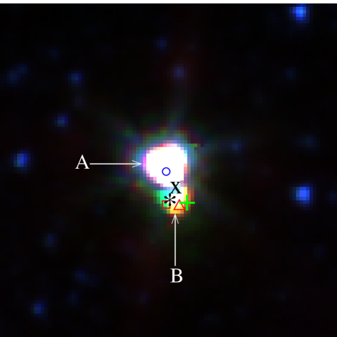
Figure 5: Spitzer-IRAC colour composite image (blue-band1, green-band2, red-band-3) a 1′$\times$1′field centred on IRAS 18345. The symbols $\circ$, $\ast$, X, +, $\square$ and $\Delta$ show the locations of the source detected by WISE at 3.4 $\mu$m and 22 $\mu$m, Spitzer-MIPS at 24 $\mu$m and 70 $\mu$m, Beuther et al. (2002a ) at 1.2 mm using IRAM 30-m telescope amd MAMBO, and and Williams et al. (williams04 (2004)) at 850 $\mu$m using JCMT and SCUBA. respectively.

2.3.1 CO ($J$=3–2) data

CO observations were performed using the JCMT in 2008. The ¹²CO (3–2) (345.796 GHz) maps were observed on 20080421 UT, while the ¹³CO (3–2) (330.588 GHz) and C¹⁸O (3–2) (329.331 GHz) maps were simultaneously observed on 20080707 UT. All observations were performed in position-switched raster-scan mode and using half array spacing with HARP (Buckle et al. buckle09 (2009)) as the front end. The ACSIS autocorrelator was used as the back end. ACSIS was setup in dual sub-band mode for the ¹³CO/C¹⁸O observations giving a bandwidth of 250 MHz and a resolution of 0.06 MHz (0.055 km s^-1) for each line. The ¹²CO data were taken in single sub-band mode with a bandwidth of 1000 MHz and a resolution of 0.488 MHz (0.42 km s^-1). The atmospheric opacity at 225 GHz, measured with the CSO dipper, was 0.26 for ¹²CO and 0.07–0.08 for ¹³CO/C¹⁸O. The telescope pointing was checked and corrected before the observations. The pointing accuracy on source is expected to be better than 2″.

The CO data were taken from the JCMT Science Archive where they had been reduced using the orac-dr pipeline. The pipeline first performs a quality-assurance check on the time-series data before trimming and de-spiking. It then applies an iterative baseline removal routine before creating the final group files.

Figure 6 shows a 3.3′$\times$3.3′field of the ¹²CO spectral cube, which shows well defined outflow. Figure 7 shows the same field in ¹³CO and C¹⁸O lines. ¹³CO (3–2) is also detected in outflow whereas in C¹⁸O, we mostly detect the emission from the central core. Figure 8 shows plots of the integrated spectra of ¹²CO, ¹³CO and C¹⁸O in a 1′$\times$1′field around IRAS 18345. The dotted-dashed vertical line shows the rest velocity of the cloud. The emission at $\sim$110 km s^-1 (Figures 6, 7 and 8) is probably not related to the outflow.

Figure 6: ¹²CO (J=3-2) spectral cubes covering a 3.3′$\times$3.3′field surrounding IRAS 18345 in a velocity range 77.6 km s^-1 to 113.5 km s^-1 centred on the CO-line rest frequency. The left and right panels show the spectral cube in two different orientations. The central panel shows the same region as in the left panel, but with the faint emission filtered out to show the outflow more clearly. The red square shows the plane of the $\upsilon$_LSR of the core. The contours representing the blue- and red-shifted outflow lobes projected on to the sky plane are shown in Fig. 1.

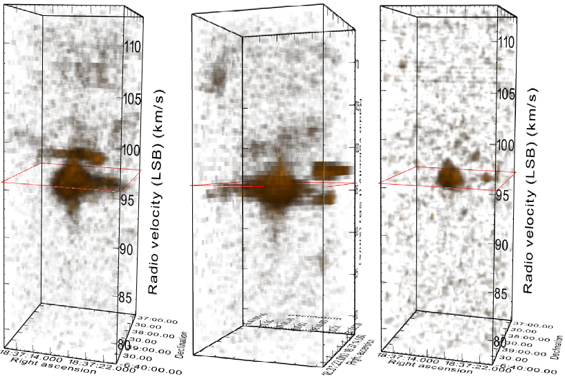
Figure 7: ¹³CO (J=3-2) and C¹⁸O (J=3-2) spectral cubes with the same spatial and spectral coverages as in Figure 6. The left and central panels show the ¹³CO cube from two different orientations and the right panel shows the C¹⁸O cube. The red square shows the plane of the $\upsilon$_LSR of the core.

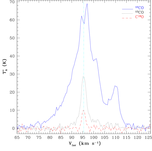
Figure 8: The ¹²CO, ¹³CO and C¹⁸O (J=3-2) spectra integrated in a 1′$\times$1′-box around IRAS 18345. The dotted-dashed vertical line at 95.5 km s^-1 shows the $\upsilon$_LSR of the core. The emission at 110 km s^-1 is from the ambient medium.

3 Results and discussion

3.1 The outflows

Through deeper observations in H₂ and $K$, we confirm the tentative detection of an H₂ outflow by Varricatt et al. (varricatt10 (2010)). The continuum subtracted H₂ image in Figure 1 shows the emission features labelled MHO 2211, which is composed of two knots directed away from ‘B’. We derive an outflow angle of 95^∘ east of north if these are produced by an outflow from a source at the location of ‘B’.

High angular resolution VLBI observations of the 6.7 GHz Class-II methanol maser by Bartkiewicz et al. (bartkiewicz09 (2009)) revealed 30 maser spots distributed in the form of an ellipse with semi-axes 103 mas and 70 mas respectively. They conclude that the 6.7 GHz methanol masers form in a disk or torus around the massive YSOs, at the interface between the disk and the outflow, and that these masers form in a stage before the formation of the UCHii region. They estimate a radius of 980 AU for the ring of distribution of the maser spots, for a distance of 9.5 kpc. The coordinates of the brightest maser spot given by Bartkiewicz et al. ($\alpha$=18:37:16.92106 $\delta$=-06:38:30.5017) agrees with those of the infrared source ‘B2’ within 0.25″. It is also noteworthy that the major axis of the ring-like distribution of the maser spots is at an angle of 90^∘, which is nearly perpendicular to the direction of orientation of the CO outflow, as it would be expected if they form in a disk or torus around the YSO. Assuming a circular distribution for the maser spots, we infer an outflow angle of 43^∘ with respect to the sky plane.

The CO (3–2) mapping using JCMT (§2.3.1) reveal a well-defined outflow (Figures 6, 8). Contours generated from the blue- and red-shifted lobes of the outflow are overlaid on the H₂ image in Figure 1. The contours start at 3 $\sigma$ above the average background level in the integrated blue and red lobes of the outflow. The outflow is oriented approximately N-S; we measure an angle of 161^∘ E of N for the blue lobe. The outflow appears to be centred on source ‘B’ and is in good agreement with the outflow from this source detected in ¹²CO (2–1) by Beuther et al. (2002b ). Figure 1 shows that the direction of this outflow detected in CO is very different when compared with an angle of 95^∘ derived for the H₂ outflow. The outflow appears to be at a high inclination with respect to the sky plane, as inferred from the overlapping blue- and red-shifted lobes (Figure 1) and the high velocity range (Figure 8); we adopt the angle of inclination of 43^∘ with respect to the sky plane inferred from the methanol masers for the calculations in this paper.

The CO spectral line data are used to determine the outflow properties. The velocity-integrated blue- and red-shifted spectral images were deconvolved using a 2D Gaussian of FWHM=14.58″, which is the beam size of the JCMT at this frequency. At 3-$\sigma$ level on the blue- and red-shifted images, the projected outflow length is 28″, and the width for the blue-shifted lobe is 47″. After correcting the observed length for an angle of inclination of 43^∘, we derive a collimation factor of 0.81 for the outflow. Using a distance of 9.5 kpc, and an average of the maximum observed velocities of the blue and red-shifted lobes of the outflow of 18 km s^-1, we derive the outflow length and dynamical time as 1.76 pc and 9.58$\times$10⁴ years respectively.

The optical depth in ¹²CO ($\tau_{12}$) can be obtained from a ratio of the antennae temperatures (T${}^{*}_{A}$) obtained in ¹²CO and ¹³CO assuming ¹²CO/¹³CO=89, and using Eq. 1 (Garden et al. garden91 (1991)).

$$\frac{T^{*}_{A}(^{12}CO)}{T^{*}_{A}(^{13}CO)}=\frac{1-e^{-\tau_{12}}}{1-e^{-\tau_{13}}}=\frac{1-e^{-\tau_{12}}}{1-e^{-\frac{\tau_{12}}{89}}}$$ (1)

Since ¹²CO suffers from self absorption near the central velocity of the line (Figure 8), we estimated $\tau$ separately in the blue and red wings adopting velocity ranges where both ¹²CO and ¹³CO were detected. We derive values of 18.85 and 15.65 for $\tau_{12}$ in the blue and red wings respectively.

The ¹²CO spectrum exhibits a strong emission component at $\sim$110 km s^-1 (Figures 6 and 8), which is probably not related to the outflow, and is arising from the ambient medium. This feature was interpolated out from the spectrum before estimating the emission in ¹²CO from the blue- and red-shifted lobes of the outflow. We used velocity ranges 77–90 km s^-1 and 102–113 km s^-1 respectively for integrating the line wing emission in the blue- and red-shifted lobes.

Following Garden et al. (garden91 (1991)), the ¹²CO column density is derived using the equation

$$N=\frac{3k}{8\pi^{3}B\mu^{2}}\frac{e^{\frac{hBJ(J+1)}{kT\textsubscript{ex}}}}{(J+1)}\frac{(T\textsubscript{ex}+\frac{hB}{3k})}{[1-e^{\frac{-h\nu}{kT\textsubscript{ex}}}]}\int\tau_{\upsilon}\leavevmode\nobreak\ d\upsilon\leavevmode\nobreak\ cm^{-1},$$ (2)

where B is the rotational constant, $\mu$ is the electric dipole moment of the molecule, $J$ is the lower level of the transition, and $T$_ex is the excitation temperature. Substituting the values for B and $\mu$ in Eq. 2,

$$N=2.39\times 10^{14}\frac{e^{\frac{hBJ(J+1)}{kT\textsubscript{ex}}}}{(J+1)}\frac{(T\textsubscript{ex}+0.92)}{[1-e^{\frac{-16.6}{T\textsubscript{ex}}}]}\int\tau_{\upsilon}\leavevmode\nobreak\ d\upsilon\leavevmode\nobreak\ cm^{-1},$$ (3)

where $\upsilon$ is in km s^-1.

Allowing for beam filling factor and ignoring the effect of the cosmic background radiation,

$$N=\frac{2.39\times 10^{14}}{16.6}\frac{e^{\frac{hBJ(J+1)}{kT\textsubscript{ex}}}}{(J+1)}\frac{(T\textsubscript{ex}+0.92)}{e^{\frac{-16.6}{T\textsubscript{ex}}}}\int\frac{T^{*}_{A}}{\eta_{b}}\frac{\tau_{\upsilon}\leavevmode\nobreak\ d\upsilon}{(1-e^{-\tau_{\upsilon}})}\leavevmode\nobreak\ cm^{-1}.$$ (4)

Adopting 30 K for $T$_ex (Beuther et al. 2002b ) and $10^{4}$ for H₂/CO, Eq. 4 yields 1.37$\times$10²¹ cm^-2 and 1.03$\times$10²¹ cm^-2 respectively for the column density of H₂ in the blue- and red-shifted lobes.

The mass in the outflow lobes can be obtained using the relation $m\leavevmode\nobreak\ \times\leavevmode\nobreak\ nH_{2}\leavevmode\nobreak\ \times\leavevmode\nobreak\ S$, where $m$ is the mean atomic weight, which is 1.36$\times$mass of the hydrogen molecule, and $S$ is the surface area of the outflow lobe (Garden et al. garden91 (1991)). At 3$\sigma$ above the mean background, we measure projected sizes (major axis $\times$ minor axis) of 55″$\times$45″and 30″$\times$22″respectively for the blue- and red-shifted lobes of the outflow. Integrating within these regions, within the velocity ranges of 77–90 km s^-1 and 102–113 km s^-1 respectively, we get 123 M_⊙ and 25 M_⊙ for the masses contained in the blue- and red-shifted lobes of the outflow. This gives a total mass of 148 M_⊙ for the material in the outflow. Using the maximum observed velocities ($\upsilon$_max) 18.5 km s^-1 and 17.5 km s^-1 respectively for the blue and red wings, and ignoring the angle of inclination of the outflow (see Cabrit & Bertout cabrit92 (1992)), we derive an outflow momentum of 2662 M_⊙ km s^-1, energy of 45$\times$10⁴⁶ ergs, and a mass entrainment rate ($\dot{M}$_out) of 15.6$\times$10^-4 M_⊙ year^-1. The total mass in the outflow estimated by us is very similar to 143 M_⊙ estimated by Beuther et al. (2002b ) from CO (2–1). However, the outflow momentum, energy and mass entrainment rate estimated by us are higher. The difference comes from the higher value of $\upsilon$_max used by us, and the outflow momentum, energy and mass entrainment rate estimated here should be treated as upper limits only.

The collimation factor $f_{c}$=0.81 we obtain from the CO (3–2) map is lower than a value of 1.5 derived by Beuther et al. (2002b ) from their CO (2–1) map observed at a higher spatial resolution. Note that the deconvolved image of the blue-shifted lobe is highly asymmetric (see the blue contours in Figure 1). If this asymmetry is due to two overlapping outflows, the collimation factor will be higher; using a width of 26″of the red-shifted outflow lobe, we get a collimation factor of 1.46. With the direction of the outflow derived from the aligned H₂ knots much different from the direction of the main outflow mapped in CO, and roughly agreeing with the direction of the asymmetry of the blue lobe of the CO outflow as seen in Figure 1, it is very likely that this region hosts at least two YSOs in outflow phase.

3.2 The sources driving the outflows

Figure 1 shows that the CO outflow is centred very close to the near-IR source ‘B’. The H₂ line emission knots (MHO 2211) also appear to be tracing back to the location of ‘B’. Figure 9 shows a ($J-H$) - ($H-K$) colour-colour diagram constructed using the objects detected in a 2′$\times$2′field around IRAS 18345. Since the UKIDSS observations were performed in better sky conditions than our current observations, UKIDSS data are used to construct the colour-colour diagram. For ‘A’ and ‘B’, the most recent magnitudes from Table 2 are used. ‘B’ for which $H$ and $J$ magnitudes are upper limits are shown with upward and rightward directed arrows to show the directions in which it move in the diagram with reliable detection in these bands. Both objects are at very large extinction. Source ‘B’ exhibits large excess and is located in the region of the colour-colour diagram occupied by luminous YSOs. The $K$-magnitudes given in Table 2, observed from 2003 to 2012 (all in the same photometric system and using the same aperture), show that ‘B’ is a variable.

The Spitzer-IRAC colour-colour diagram is useful to identify YSOs. Figure 10 shows the colours of objects detected in the IRAC images, within a 10′$\times$10′field around IRAS 18345. The dashed horizontal line shows the boundary between Class I/II (below) and Class I objects (above), and the dotted red arrows show reddening vectors for A_V = 50 derived using the extinction law given in Mathis (1990). Objects with ([3.6]-[4.5])$>$0.8 and ([5.8]-[8.0])$>$1.1 are likely to be Class I objects, which are protostars with infalling envelopes. Those with 0$<$([3.6]-[4.5])$<$0.8 and 0.4$<$([5.8]-[8.0])$<$1.1, within the region shown by the rectangle, are likely to be Class II objects, which are stars with discs. Most of the objects are located around ([5.8]-[8.0], [3.6]-[4.5]) = 0, which are foreground and background stars and discless pre-main-sequence (Class III) objects (Allen et al. allen04 (2004); Megeath et al. megeath04 (2004); Qiu et al. qiu08 (2008)). Locations of ‘A’ and ‘B’ are shown by filled red-circles in Figure 10. Source “A” is located in the region occupied by young sources with discs and large reddening, and ‘B’ is located in the region of even younger sources at larger reddening and an infalling envelopes. However, note that the locations of these objects could be affected by saturation, especially in the 8$\mu$m band. The locations of the two sources in Figures 9 and 10 suggest that ‘B’ is younger than ‘A’.

All data available with good spatial resolution (UKIRT-$J,H,K,L^{\prime},M^{\prime}$ and 12.5 $\mu$m and Spitzer-IRAC) data show that source ‘B’ has a steeper SED than ‘A’. At 12.5 $\mu$m, ‘B’ contributes 25.6% of the total flux of ‘A’ and ‘B’ combined, whereas in $L^{\prime}$ (3.75 $\mu$m) and $M^{\prime}$ (4.7 $\mu$m), ‘B’ contributes only 4.3% and 12.4% respectively of total flux of ‘A’ and ‘B’ combined. At shorter wavelengths (UKIRT, Spitzer-IRAC and WISE 3.4 $\mu$m), ‘A’ is the leading source. The longer wavelength observations (Spitzer-MIPS, WISE-24 $\mu$m, JCMT and IRAM) do not have the spatial resolution to resolve ‘A’ and ‘B’. However, the excellent positional accuracies of these observations enable us to identify the leading YSO with good confidence. Figure 5 shows a colour composite image of a 1′$\times$1′field surrounding IRAS 18345, constructed from Spitzer-IRAC images in bands 1, 2 and 3. Locations of sources detected in different observations with good positional accuracies are overlaid on the image. As can be seen in Figure 5 all longer wavelength observations peak near source ‘B’. These factors leads us to infer that ‘B (B1+B2)’ or some embedded sources very close to it are the YSOs responsible for the outflows in this system.

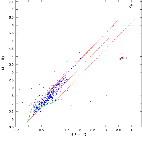
Figure 9: WFCAM $JHK$ colour-colour diagram of a 2′$\times$2′region surrounding IRAS 18345; UKIDSS data obtained in better sky conditions are used. The blue dots show the colours of point sources detected. The red dots are the colours of sources ‘A’ and ‘B’ derived from the most recent observations. The continuous green lines show the colours of unreddened main sequence and red-giant stars taken from Tokunaga et al. (tokunaga00 (2000)). The long-dashed green line shows the loci of CTTS from Meyer et al. (meyer97 (1997)). The long red arrows show the reddening vectors for A_V $\leq$ 50 derived from the interstellar extinction law given by Rieke & Lebofsky (1985).

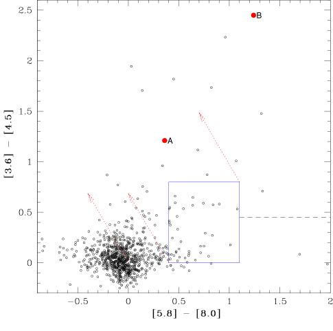
Figure 10: The IRAC colour-colour diagram. The open (black) circles show the objects detected in all four IRAC bands in a 10$\arcmin\times$10$\arcmin$ field centred on IRAS 18345. The locations of sources ‘A” and “B” are shown by filled (red) circles. The loci of Class II sources are shown by the blue rectangle; the dashed horizontal line shows the boundary between Class I/II objects (below) and Class I objects (above). The dotted red arrows show reddening vectors for A_V=50.

3.2.1 The spectral energy distribution

We modelled the SED of IRAS 18345 using the SED fitting tool of Robitaille et al. (robitaille07 (2007)), which uses a grid of 2D radiative transfer models presented in Robitaille et al. (robitaille06 (2006)), developed by Whitney et al. (2003a , 2003b , etc). The grid consists of SEDs of 20000 YSO models covering a range of stellar masses from 0.1 to 50 M_⊙ and and evolutionary stages from the early envelope infall stage to the late disc-only stage, each at 10 different viewing angles. With all the longer wavelength data peaking close to ‘B’, we have treated that as the leading YSO in this region.

Up to 12.5 $\mu$m, we have fluxes of ‘B’ available. WFCAM $K$, IRCAM $L^{\prime}M^{\prime}$, Spitzer-IRAC Bands 1 and 3 and MICHELLE 12.5-$\mu$m flux of ‘B’ were used. WFCAM $H$ magnitude was not used since in $H$, we are probably seeing only the nebulosity associated with ‘B’. Spitzer-IRAC Bands 2 and 4 fluxes were not used since they are near saturation. The resolution of WISE images is not sufficient to resolve the two sources, so WISE 3.4–12-$\mu$m data were not used to construct the SED. At 22 $\mu$m, the WISE source is located close to ‘B’, there is still likely to be a significant contribution to the flux from ‘A’. Hence the 22-$\mu$m flux was used as an upper limit. IRAS catalog lists the flux values for IRAS 18345 in 12 and 100 $\mu$m bands as lower limits, and the 100-$\mu$m flux may be affected by infrared cirrus, so those values were not used in the SED analysis. AKARI-IRC 9-$\mu$m flux was not used since that wavelength was already covered by the higher resolution UKIRT data. Similarly, MSX data in Bands A, C and D were not used. AKARI-IRC 18-$\mu$m data and MSX Band-E data are treated as upper limits only since they contain contributions from source ‘A’. The large bandwidths of the IRAS and AKARI photometry warrant colour corrections, which were performed using the correction factors given in their respective point source catalogs (Beichman et al. beichman88 (1988); Kataza et al. kataza10 (2010); Yamamura et al. yamamura10 (2010)). The JCMT-SCUBA 450 and 850-$\mu$m fluxes were adopted from Williams, Fuller & Sridharan (williams04 (2004)). Flux estimates at 1.1 mm and 1.2 mm were adopted from Rosolowsky et al. (rosolowsky10 (2010)) and Beuther et al. (2002a ) respectively. Figure 11 shows the model fit to the spectral energy distribution. Table 5 shows the results of the SED modelling. The model fit to the SED yields a very young object of mass 19.8 M_⊙, age 3.3$\times$10³ years and luminosity 1.9$\times$10⁴ L$\odot$. Figure 11 shows that there is a large disagreement between the fluxes obtained by different telescopes in the wavelength range of 60–140 $\mu$m. The flux estimated from the Spitzer-MIPS 70 $\mu$m image is much lower than what was seen in IRAS 60 $\mu$m and AKARI 66 $\mu$m bands. Similarly, the AKARI 90 and 140-$\mu$m fluxes also deviate significantly from the model SED. Inadequate spatial resolution and the different contributions from the background could be severely affecting the fluxes measured in these bands used by telescopes of different sizes and spatial resolutions. The SED analysis for this source available in the literature, performed using the same model (Tanti, Roy & Duorah, tanti11 (2011)) using all the available data, obtained a 12.99 M_⊙ YSO with an age of 1.36$\times$10⁴ years and a luminosity of 7.21$\times$10³ L_⊙. The difference mostly comes from the fact that they do not attempt to separate the fluxes of ‘A’ and ‘B’.

The results obtained from our SED analysis bring some complications. The dynamical time scale of the outflow (9.58$\times$10⁴ years) derived by us from the CO (3–2) data is much larger than the age of the YSO (3.3$\times$10³ years) obtained from the SED analysis. This is unrealistic. This discrepancy may mostly be caused by the contribution from a companion at longer wavelengths, thereby making the star appear younger. We have removed the contributions from source ‘A’ to the total flux for wavelengths up to 12.5 $\mu$m. The centroids of all detections at longer wavelengths are located close to ‘B’, hence ‘A’ is not likely to be the main contributor at longer wavelengths. The more probable chance is that ‘B’ itself is a binary or multiple as strongly suggested by its resolution into two components ‘B1’ and ‘B2’ in $L^{\prime}$ and $M^{\prime}$, and the detection of outflows with two different directions from H₂ and CO observations, both of which appear to be centred near ‘B’. High-angular-resolution observations at longer wavelengths are therefore required to properly understand the complexity of the star formation taking place here.

Figure 11: The SED of IRAS 18345. The filled circles show the data in WFCAM $K$ band, IRCAM $L^{\prime}$ and $M^{\prime}$ bands, Spitzer-IRAC Bands 1 and 3, Michelle 12.5 $\mu$m, IRAS 60 $\mu$m, AKARI at 65–140 $\mu$m, Spitzer-MIPS 70 $\mu$m, SCUBA 450 and 850 $\mu$m, Bolocam 269 GHz and IRAM 240 GHz data. The downward-directed triangles show AKARI-IRC 18 $\mu$m, MSX band-E and WISE band-4 data which are treated as upper limits. The continuous line shows the best fit model. The grey lines show subsequent good fits for ($\chi^{2}-\chi^{2}_{bestfit}$) per data point $<$ 3. The dashed line corresponds to the stellar photosphere for the central source of the best fitting model, as it would look in the absence of circumstellar dust (but including interstellar extinction).

Table 5: Results from the SED fitting

Parameter	Best-fit valuesa
Stellar mass (M⊙)	19.8 (+3, -1.5)
Stellar age (yr)	3.3 (+.49, -0.77)$\times$103
Stellar radius (R${}_{\odot})$	230 (+16, -20)
Stellar temperature (K)	4480 (+260, -167)
Disk mass (M⊙)	1.9 (+6, -0)$\times$10-1
Disk accretion rate (M⊙yr-1)	2.5 (+4, -1.4)$\times$10-5
Disk/envelope inner radius (AU)	9.9 (+0, -1.3)
Disk outer radius (AU)	11.7 (+11.8, -0)
Envelope mass (M⊙)	2.2 (+3.6, -0)$\times$103
Envelope accretion rate (M⊙yr-1)	4.1 (+4.3, -0.2)$\times$10-3
Envelope outer radius (AU)	1 (+0, -0.4)$\times$105
Total Luminosity (L⊙)	1.9 (+2, -1.5)$\times$104
AV circumstellar (mag)	804 (+508, -453)
AV interstellar (mag)	25 ($\pm$13)
Angle of inclination of the disk axis (∘)	18

• The values given in parenthesis are the rms of the differences, in parameter values of models with ($\chi^{2}-\chi^{2}_{bestfit}$) per data point $<$ 3, above and below those of the best-fit model, estimated with respect to the parameter values of the best-fit model. A distance of 9.5 kpc is adopted.

4 Conclusions

1. IRAS 18345 is a very young massive YSO in a phase of active accretion.

2. Through near and mid-IR observations, we identify the central source, which is highly obscured and is probably double at a separation of $\sim$0.45″.

3. We confirm the 2.122 $\mu$m H₂ outflow tentatively detected by Varricatt et al. (varricatt10 (2010)). The direction of this outflow is very different from the direction of the main outflow mapped in CO. The origins of both H₂ and CO outflows appear to trace back to the location of the infrared source mentioned above. In addition, the SED analysis does not fit well with a single YSO model. This suggests that more than one YSO are driving outflows here.

4. The SED analysis yields a 19.8 M_⊙ star of age 3.3 $\times$10³ years. The age is far lower than what is implied by the dynamical time of the outflow. The unresolved binarity is probably the factor affecting the SED analysis, resulting in an overestimate of the mass and underestimate of the age.

5. The collimation factor of the outflow derived by us from the CO (3-2) maps is low (0.81). It needs to be explored if this is real, or is due to the presence of more than one outflow.

6. We emphasize the need high-angular-resolution observations at mid-IR and longer wavelengths to properly understand this system, and in general massive star forming regions. High angular resolution interferometric CO line observations are also required to understand if the apparently single outflow seen in CO is composed of more than one component.

- (1) Allen, L. E. et al. 2004, ApJS, 154, 363
- (2) Anderson, T., De Lucia, Fr, Herbst, E. 1990, ApJS, 72, 797
- (3) Arce, H. G., Shepherd, D., Gueth, F., Lee, C.-F., Bachiller, R., Rosen, A., Beuther, H. 2007, Protostars and Planets V, 245
- (4) Beichman, C. A.; Neugebauer, G., Habing, H. J., Clegg, P. E., Chester, T. J. 1988, iras, 1
- (5) Bartkiewicz, A., Szymczak, M., van Langevelde, H. J., Richards, A. M. S., Pihlström, Y. M. 2009, A&A, 502, 155
- (6) Beuther, H., Schilke, P., Menten, K. M., Motte, F., Sridharan, T. K., Wyrowski, F. 2002a, ApJ, 566, 945
- (7) Beuther, H., Schilke, P., Sridharan, T. K., Menten, K. M., Walmsley, C. M., Wyrowski, F. 2002b, A&A, 383, 892
- (8) Beuther, H., Walsh, A., Schilke, P., Sridharan, T. K., Menten, K. M., Wyrowski, F. 2002c, A&A, 390, 289
- (9) Bronfman, L., Nyman, L. A., May, J. 1996, A&AS, 115, 81
- (10) Buckle, J. V., Hills, R. E., Smith, H., and 35 coauthors 2009, MNRAS, 399, 1026
- (11) Cabrit, S., Bertout, C. 1992, A&A, 261, 274
- (12) Casali, M. et al. 2007, A&A, 467, 777
- (13) Cavanagh, B., Jenness, T., Economou, F., Currie, M. J. 2008AN….329..295C
- (14) Currie M. J., Draper P. W., Berry D. S., Jenness T., Cavanagh B., Economou F. 2008, in Argyle R. W., Bunclark P. S., Lewis J. R., eds., Astron. Soc. of the Pac. Conf. Series Vol. 394, Astronomical Data Analysis Software and Systems XVII. p. 650
- (15) Davis, C. J., Varricatt, W. P., Todd, S. P., Ramsay Howat, S. K., 2004, A&A, 425, 981
- (16) Doi, Y., Etxaluze Azkonaga, M., White, G., et al. 2009, sitc.conf, p.4018
- (17) Edris, K. A., Fuller, G. A., Cohen, R. J. 2007, A&A, 465, 865
- (18) Fazio, G. G. et al. 2004, ApJS, 154, 10
- (19) Felli, M., Palagi, F., Tofani, G. 1992, A&A, 255, 293
- (20) Garden, R. P., Hayashi, M., Hasegawa, T., Gatley, I., Kaifu, N. 1991, ApJ, 374, 540
- (21) Glasse, A. C., Atad-Ettedgui, E. I., Harris, J. W. 1997, SPIE, 2871, 1197 (Proc. SPIE Vol. 2871, p. 1197-1203, Optical Telescopes of Today and Tomorrow, Arne L. Ardeberg; Ed.)
- (22) Hambly, N. C.; Collins, R. S.; Cross, N. J. G., and 14 co authors 2008, MNRAS, 384, 637
- (23) Hewett, P. C., Warren, S. J., Leggett, S. K., Hodgkin, S. T. 2006, MNRAS, 367, 454
- (24) Hodgkin, S. T., Irwin, M. J., Hewett, P. C., Warren, S. J. 2009, MNRAS, 394, 675
- (25) Hofner, P., Kurtz, S., Ellingsen, S. P., Menten, K. M., Wyrowski, F., Araya, E. D., Loinard, L., Rodríguez, L. F., Cesaroni, R. 2011, ApJ, 739, L17
- (26) Irwin, M. J., Lewis, J., Hodgkin, S., et al. 2004, in Optimizing Scientific Return for Astronomy through Information Technologies, eds. P. J. Quinn & A. Bridger, Proc. SPIE, 5493, 411
- (27) Ishihara, D., Onaka, T., Kataza, H., and 30 co-authors 2010, A&A, 514A, 1
- (28) Kataza, H. et al. 2010, AKARI-IRC Point Source Catalogue Release note Version 1.0
- (29) Lawrence, A., Warren, S. J., Almaini, O., and 19 co authors 2007, MNRAS, 379, 1599
- (30) Maret, S., Ceccarelli, C., Tielens, A. G. G. M., Caux, E., Lefloch, B., Faure, A., Castets, A., Flower, D. R. 2005, A&A, 442, 527
- (31) Mathis, J. S. 1990, ARA&A, 28, 37
- (32) Megeath, S. T. et al. 2004, ApJS, 154, 367
- (33) Meyer, M. R., Calvet, N., Hillenbrand, L. A. 1997, AJ, 114, 288
- (34) Murakami, H. et al. 2007, PASJ, 59, S369
- (35) Pestalozzi, M. R., Minier, V., Booth, R. S. 2005, A&A, 432, 737
- (36) Prestage, R. M, Meyerdierks, H., Lightfoot, J. F, Jenness, T., Tilanus, R. P. J, Padman R. 2000, specx - A Millimetre Wave Spectral Reduction Package, CCLRC / Rutherford Appleton Laboratory, Particle Physics & Astronomy Research Council, Starlink User Note 17.8
- (37) Qiu, K. et al. 2008, ApJ, 685, 1005
- (38) Rieke, G. H. et al. 2004, ApJS, 154, 25
- (39) Rieke, G. H., Lebofsky, M. J. 1985, ApJ, 288, 618
- (40) Robitaille, T. P., Whitney, B. A., Indebetouw, R., Wood, K., and Denzmore, P. 2006, ApJS, 167, 256
- (41) Robitaille, T. P., Whitney, B. A., Indebetouw, R., Wood, K. 2007, ApJS, 169, 328
- (42) Rodgers, S. D., Charnley, S. B. 2003, ApJ, 585, 355
- (43) Rosolowsky, E., Dunham, M. K., Ginsburg, A., Bradley, E. T., Aguirre, J., Bally, J., Battersby, C., Cyganowski, C., Dowell, D., Drosback, M., and 6 coauthors 2010, ApJS, 188, 123
- (44) Sridharan, T. K., Beuther, H., Schilke, P., Menten, K. M., Wyrowski, F. 2002, ApJ, 566, 931
- (45) Szymczak, M., Hrynek, G., Kus, A. J. 2000, A&AS, 143, 269
- (46) Szymczak, M., Kus, A. J., Hrynek, G., Kĕpa, A., Pazderski, E. 2002, A&A, 392, 277
- (47) Tanti, K. K, Roy, J., Duorah, K. 2011, IJSER, Vol. 2, Issue 10
- (48) Thomas, H. S., Fuller, G. A. 2008, A&A, 479, 751
- (49) Tokunaga, A. T. 2000, in Allen’s Astrophysical Quantities, ed. A. N. Cox (Springer-Verlag), 143
- (50) van der Walt, D. J., Gaylard, M. J., MacLeod, G. C. 1995, A&AS, 110, 81
- (51) Varricatt, W. P., Davis, C. J., Ramsay, S., Todd, S. P. 2010, MNRAS, 404, 661
- (52) Whitney, B. A., Wood, K., Bjorkman, J. E., Cohen, M. 2003a, ApJ, 598, 1079
- (53) Whitney, B. A., Wood, K., Bjorkman, J. E., Wolff, M. J. 2003b, ApJ, 591, 1049
- (54) Williams, S. J., Fuller, G. A., Sridharan, T. K. 2004, A&A, 417, 115
- (55) Wright, E. L., Eisenhardt, P. R. M., Mainzer, A. K., et al. 2010, AJ, 140, 1868
- (56) Yamamura, I., Makiuti, S., Ikeda, N., Fukuda, Y, Oyabu, S, Koga, T., White, G. J. 2010, AKARI-FIS Bright Source Catalogue Release note Version 1.0