Determination of the axial and pseudoscalar form factors from lattice QCD
Abstract
We present a lattice QCD calculation of the matrix elements of the axial-vector and pseudoscalar currents. The decomposition of these matrix elements into the appropriate Lorentz invariant form factors is carried out and the techniques to calculate the form factors are developed and tested using quenched configurations. Results are obtained for domain wall fermions and within a hybrid scheme with domain wall valence and staggered sea quarks. Two Goldberger-Treiman type relations connecting the axial to the pseudoscalar effective couplings are derived. These and further relations based on the pion-pole dominance hypothesis are examined using the lattice QCD results, finding support for their validity. Utilizing lattice QCD results on the axial charges of the nucleon and the , as well as the nucleon-to- transition coupling constant, we perform a combined chiral fit to all three quantities and study their pion mass dependence as the chiral limit is approached.
I INTRODUCTION
Great progress has been made in lattice QCD studies of hadron spectroscopy and structure and lattice QCD results are beginning to provide input to phenomenology and experiment. Simulations with dynamical quarks near and at the physical pion mass Jansen (2008); Durr et al. (2008); Aoki et al. (2009); Durr et al. (2011) have been shown to produce the observed low-lying hadron spectrum Durr et al. (2008); Alexandrou et al. (2009a); Aoki et al. (2010) and scattering lengths have been calculated to good accuracy Beane et al. (2012); Dudek et al. (2012); Feng et al. (2010); Yamazaki et al. (2004).
Whereas producing experimentally measured quantities from first principles provides a powerful validation of the lattice QCD methodology, calculating quantities that are difficult to extract or have impact in probing physics beyond the standard model is a much more challenging prospective. Studying the structure of the resonance is an example of the input lattice QCD can provide to phenomenology that cannot be directly extracted from experiments. This is because the decays strongly with a lifetime of seconds Kotulla et al. (2002); Lopez Castro and Mariano (2001) and resists experimental probing. Measurements of the magnetic moment exist albeit with a large experimental uncertainty. The , having width MeV and lying close to the threshold, plays an important role in chiral expansions. In heavy baryon chiral perturbation theory it has been included as an explicit degree of freedom Bernard et al. (2005); Hemmert et al. (1998); Jenkins and Manohar (1991); Fettes and Meissner (2001), where it is argued that it improves chiral expansions applied in the description of lattice QCD results such as the nucleon axial charge Hemmert et al. (2003). Chiral langragians with degrees of freedom involve additional coupling constants that are difficult to measure. Therefore, one either treats them as free parameters to be fitted along other parameters using lattice QCD results Bernard et al. (2005); Bernard (2008) and data extracted from partial-wave analysis of scattering measurements Jenkins and Manohar (1991); Fettes and Meissner (2001) or estimates them based on phenomenology and symmetries. For example, one can relate the nucleon axial charge , which is well measured, to the axial charge, in the large- limit Dashen et al. (1994) or using symmetry Brown and Weise (1975). The Goldberger-Treiman (GT) relation is then used to get the effective coupling. Another framework to extract the coupling is via sum rules Choi et al. (2010).
Lattice QCD provides a nice framework to study the properties and calculate the coupling constants. In some of our recent work we developed the formalism to study the transition form-factors within lattice QCD Alexandrou et al. (2007); Alexandrou et al. (2011a), as well as the electromagnetic form-factors Alexandrou et al. (2009b). The quadrupole electromagnetic form factor, extracted for the first time, provided input for the deformation of the showing that in the infinite momentum frame the is prolate Alexandrou et al. (2012).
In this work, we present a detailed study of the axial-vector and pseudoscalar form factors of the . The theoretical framework and a subset of the results were given in Ref. Alexandrou et al. (2011b). Here we discuss in detail the lattice techniques developed and utilized for the extraction of these form factors. In addition, we present an extended analysis of the momentum dependence of all the form factors using an additional ensemble of dynamical domain wall fermions. We also include a study of the pion-pole dominance predictions and compare them to our lattice QCD results.
The outline of the paper is as follows: In Section II we present the decomposition of the matrix elements of the axial-vector and pseudoscalar currents. In Section III we explain our lattice techniques and discuss the ensembles utilized for the calculation. In Section IV we present the lattice results on all form factors and examine several relations among them and their phenomenological consequences. In Section V we perform a combined chiral fit using our results on the nucleon axial charge Alexandrou et al. (2011c), the axial charge calculated in this work and the dominant axial transition form factor, , calculated in previous work on the same sets of lattices Alexandrou et al. (2011a). Finally, in Section VI we give a summary and conclusions. Technical details and our values on the form factors are presented in the Appendices.
II The Axial and Pseudoscalar Matrix Element of the
Lorentz invariance and spin-parity rules determine the decomposition of the matrix element of the isovector axial-vector current in terms of four invariant functions of the momentum transfer squared, :
| (1) |
where denotes the initial momentum (spin) of the and the final momentum (spin). The flavor-isovector axial-vector current operator is defined as
| (2) |
where denotes the Pauli matrix acting in flavor space and is the isospin quark doublet. The four axial form factors, and as defined in Eq. (1) are grouped into the familiar structure of the nucleon axial-vector vertex.
In the description of spin-3/2 energy-momentum eigenstates, classical solutions of the Rarita-Schwinger equation play a central role. Each component of a vector-spinor , with a Lorentz four-vector index solves the free Dirac equation
| (3) |
Implementing additionally the constraint equations,
| (4) |
the unphysical components are eliminated and the remaining eight degrees of freedom describe a spin-3/2 (anti-)particle. Rarita-Schwinger spinors satisfy the spin sum relation:
| (5) | |||||
where the normalization is assumed.
The zero momentum transfer limit of (1) defines the axial charge, of the multiplet. Ref Jiang and Tiburzi (2008a) normalizes the axial charge via
| (6) |
where encodes the spin structure of the forward matrix element
| (7) |
Following the above normalization we establish via Eq. (1):
| (8) |
We note that while the Lorentz decomposition of the axial current is naturally expressed via and as in Eq.(1), a decomposition in terms of multipoles is possible as for example in the case of the electromagnetic transition Alexandrou et al. (2009b). Such a representation is more easily expressed in the Breit frame. This decomposition is performed in Appendix A in terms of four multipoles, and , and their relation to the form factors and is given.
The matrix element of the pseudoscalar density operator
| (9) |
is decomposed in terms of two Lorentz invariant form factors, denoted by and :
| (10) |
While and are the directly computable form factors from the three-point pseudoscalar correlator, they can be related to the phenomenologically more interesting pion- vertex using the partially conserved axial current hypothesis (PCAC). Using PCAC on the hadronic level one can write
| (11) |
with denoting the isotriplet pion field operator. In the SU(2) symmetric limit of QCD with denoting the up/down mass, the pseudo-scalar density is related to the divergence of the axial-vector current through the axial Ward-Takahashi identity (AWI)
| (12) |
with operators now defined as quark bilinears. Using the relations of Eqs. (11) and (12) we identify the physically relevant pion-- from factor , which at gives the coupling, as well as a second form factor , by rewriting the pseudoscalar matrix element as
| (13) |
where we effectively make the identification
| (14) | |||||
| (15) |
At zero momentum transfer only can be extracted. This coupling is analogous to the known pseudoscalar coupling constant defined for the nucleon. For the discussion presented in the next section it is useful to recall the definition of the corresponding quantities in the nucleon sector Alexandrou et al. (2007). For the matrix elements of the axial-vector current we have
| (16) |
and for the pseudoscalar density
| (17) |
Note that we have dropped for simplicity an overall kinematical factor arising from the normalization of lattice states, since it is of no relevance for our discussion here.
II.1 Goldberger-Treiman Relations
In this section we apply PCAC to derive GT relations for the . We recall that PCAC has been shown to apply satisfactorily in the nucleon case leading to the Goldberger-Treiman (GT) relation. This can be derived from Eqs. (16) and (17) related by AWI and taking to obtain in terms of the nucleon axial charge via the relation
| (18) |
Assuming varies smoothly with so that then the GT relates the physical coupling constant with the nucleon axial charge . At the chiral limit, using one derives that . Therefore, measures the chiral symmetry breaking. PCAC dictates that the form factor has a pion pole given by . The validity of the GT relation and the momentum dependence of in the nucleon case has been studied in Ref. Alexandrou et al. (2007). Similarly, a non-diagonal GT relation, applicable to the axial -to- transition is formulated and relates the axial coupling to the effective coupling. Lattice calculations examined the validity of the non-diagonal GT relation using the same ensembles as in this work Alexandrou et al. (2011a).
One can similarly derive GT relations for the by taking the matrix elements of the AWI with states, . Taking the dot-product of with the matrix element of the axial-vector current given in Eq. (1) we obtain
One possible linear combination of Eqs. (20) and (21) can be obtained by taking the dot product of Eq. (19) with leading to
| (22) |
which can be considered as a generalized GT-type relation connecting all the six form factors. At and assuming all terms in Eq. (22) are finite we obtain
| (23) |
If is a continuous slow varying function of as then and we thus derive a GT relation for the analogous to the one for the nucleon case.
Using Eq. 20 and setting we obtain a second GT relation
| (24) |
If one invokes pion-pole dominance and noting that and are both finite at the origin, it follows from Eqs. (21, 20) that as and must have a pole at . We thus arrive at the relations
| (25) |
and
| (26) |
It is thus interesting to note how the spin-3/2 nature of the state combined with PCAC leads to a pair of Goldberger-Treiman relations, given by Eqs. (23) and (24). Let us examine further these relations at the chiral limit. From Eq. (22) we find that
| (27) |
which means that in the limit the leadin behavior of , via Eq. (20) and via Eq. (26). Therefore, the second GT-type relation given in Eq. (24) cannot be extrapolated to physical pion mass since the assumption that and are slowly varying functions of no longer holds. However, since they both display a pion-pole behaviour one can factor it out on both sides and thus the ratio can be extrapolated to the physical pion. In this sense, this constitutes a second GT relation.
III LATTICE EVALUATION
III.1 Euclidean Correlators and Form Factors
Standard techniques are employed on the Euclidean space-time lattice for the evaluation of hadronic form factors. The following two-point and three-point functions are required:
| (28) |
where and are the lattice pseudoscalar or axial current insertions, and is the standard lattice interpolating field with overlap with the quantum numbers:
| (29) |
The overlap of with the spin-3/2 is
| (30) |
We will use the following matrices, which project onto positive parity for zero momentum, for our calculation
| (31) |
The Fourier transforms in (III.1) enforce a static sink at the timeslice and a momentum transfer injected via the operator insertion at an intermediate timeslice .
We insert into these correlators complete sets of hadronic energy momentum eigenstates:
| (32) |
where with we denote collectively all quantum numbers including spin. For large Euclidean time separations and the ground state propagation dominates the correlator:
| (33) | |||||
The Wick-rotated axial and pseudoscalar operators take the form
| (34) |
| (35) |
with the Euclidean four-momentum transfer . The Rarita-Schwinger spin-sum relation becomes
| (36) |
where all the matrices are in Euclidean space: and .
Forming an appropriate ratio of the 3-point to the 2-point correlator serves to cancel out the unknown -factors and leading time-dependence. A particular product of 2-point correlators which minimizes the denominator noise-level is utilized as it contains smaller time-extents. The proposed ratios are:
| (37) |
and
| (38) |
for the axial and pseudoscalar vertices. Summation over is implicit in the 2-point correlators. At large Euclidean time separations and these ratios become time-independent (plateau region).
| (39) |
where stands for the axial or pseudoscalar current. It is easy to show that the 2-point correlators are dominated by
| (40) |
and therefore the constant is determined as
| (41) |
There are at most 256 available combinations of the Dirac and Lorentz indices in Equation (39), each one expressed as a linear combination of the axial (pseudoscalar) form factors times kinematical tensor coefficients. Since we are interested in the momentum dependence of the matrix elements, evaluation of the 3-point correlators is required for a large set of transition momenta for both and operators. In order to perform this economically we utilize the sequential inversion through the sink technique Alexandrou et al. (2009b) by fixing the sink timeslice and performing a backward sequential inversion through the sink. The sequential vector is coupled with a forward quark propagator and the Fourier transformed insertion operator at all intermediate time-slices at a small computational cost, obtaining thus the full momentum dependence of the amplitude. A drawback in this approach is the fact that the quantum numbers of the source and sink interpolators –which correspond to the Lorentz indices and are now fixed per sequential inversion. Within the space of 64 available 3-point correlators corresponding to choices of and we perform an optimization by forming appropriate linear combinations such as the degree of rotational symmetry of the summed correlator is maximal and consequently all transition momentum vectors that correspond to a fixed virtuality will contribute to the form factor measurement in a rotationally symmetric fashion. This optimization technique has proved extremely useful in obtaining high accuracy results in the Nucleon elastic, Nucleon-to- electromagnetic Alexandrou et al. (2011a), axial and pseudoscalar transitions Alexandrou et al. (2007) as well as the electromagnetic form factors Alexandrou et al. (2009b). We evaluate the Dirac traces in Eq. (39) using symbolic software such as form for and Mathematica.
We construct the following two optimal linear combinations, which we refer to as Type-I and Type-II.
| (42) | |||||
| (43) |
with the matrix :
| (44) |
Detailed expressions for the decomposition of the above combinations to the four axial form factors are provided in Appendix B. The above types are in addition utilized for the extraction of the two pseudoscalar couplings (Appendix B). A large number ( correlators of axial and pseudoscalar insertion momenta are combined for momentum transfers ranging up to GeV2 per ensemble. We stress that only two sequential inversions through sink –one for each Type above– are required in order to disentangle completely all six form factors from the relevant 3-point functions.
Correlators corresponding to a fixed momentum transfer are analyzed simultaneously in an overconstrained system analysis for the extraction of the form factors. Typically plateau averages for the optimal ratios given in Eq. (39) will contribute to the determination of the form factor for each value. A global -minimization amounts technically to the singular value decomposition of an over-complete linear system, with unknowns (4 for the axial or 2 for the pseudoscalar) and input data (the O(20-50) plateau averages). Further details on this kind of analysis can be found in Ref Tsapalis (2006). Jackknife estimates are utilized for all levels of variance extraction on observables.
III.2 Ensembles and Parameters
In Table 1 we summarize the parameters and number of configurations for the ensembles used in this work. As can be seen, three sets are employed. These are the same as the ones we used previously for the study of the nucleon axial form factors as well as the nucleon-to- axial transition form factors. Therefore, these ensembles provide a complete calculation of the nucleon/ sector, allowing a direct extraction of low energy couplings from a combined fit.
| V | stat. | (GeV) | (GeV) | (GeV) | |
| Quenched Wilson fermions | |||||
| GeV | |||||
| 200 | 0.563(4) | 1.267(11) | 1.470(15) | 0.1554 | |
| 200 | 0.490(4) | 1.190(13) | 1.425(16) | 0.1558 | |
| 200 | 0.411(4) | 1.109(13) | 1.382(19) | 0.1562 | |
| Mixed action, GeV | |||||
| Asqtad (), DWF () | |||||
| 264 | 0.498(3) | 1.261(17) | 1.589(35) | ||
| Asqtad (), DWF () | |||||
| 550 | 0.353(2) | 1.191(19) | 1.533(27) | ||
| Domain Wall Fermions (DWF) | |||||
| , GeV | |||||
| 1428 | 0.297(5) | 1.27(9) | 1.455(17) | ||
The gauge configurations used in the analysis include a set of quenched configurations on a , at , corresponding to a lattice spacing fm with pion masses 560 MeV, 490 MeV and 411 MeV. The low statistical noise makes this ensemble appropriate for checking our lattice methodology and some of the phenomenological relations. We apply Gaussian smearing at the source and sink in order to minimize the excited state contamination on the baryon correlators. The parameters and have been tuned to provide optimal overlap to a nucleon state Alexandrou et al. (2007). The source-sink separation is set at fm. In our previous studies involving the such a time separation was found sufficient for ground state dominance. The second set consists of two ensembles that use two degenerate light and one strange () Asqtad-improved dynamical staggered fermions generated by the MILC collaboration Bernard et al. (2001). The strange quark mass is fixed to its physical value, the lattice spacing is set to 0.124 fm and the lowest pion mass is 353 MeV. Our calculation employs Domain Wall (DW) valence quarks with light quark mass tuned so as the pion mass matches the lowest pion mass obtained using staggered fermions. The extent of the fifth dimension of the domain wall action is set to , which was demonstrated to provide minimal violations to the chiral symmetry properties of the domain wall fermion (DWF) operator. The source-sink separation is set to fm and Gaussian smearing is applied at the source and sink with APE smearing on gauge links that enter the smearing function applied on the interpolating fields. The parameters are given in Ref. Alexandrou et al. (2007). Finally, the third set is an ensemble of DWF generated by the RBC-UKQCD collaborations Aoki et al. (2011) with a lattice spacing fm and the physical volume of and pion mass of 0.297 MeV. The extent of the fifth dimension is also here . It turns out that the residual quark mass introduced via the chiral symmetry breaking effects is , or of the bare quark mass. The smearing parameters for the interpolating fields are given in Ref. Alexandrou et al. (2011a). The sink-source time separation is set at fm. In order to increase the statistics at this lowest pion mass we use the coherent sink technique, employed in our study of the nucleon to transition using the same ensemble Alexandrou et al. (2011a). The four quark sources are placed at timeslice for each configuration. Four forward propagators must be computed – each with a source at one of the time-slices. The sinks are constructed at all four equally spaced time-slices and one sequential inversion is performed in order to construct the three-point correlator. Gauge invariance ensures that combining the sequential vector with each one of the forward quark propagators generated at , projects the appropriate matrix element between and as the other cross-terms will average to zero. It has been shown in Ref. Alexandrou et al. (2011a) that while statistics is thus multiplied by 4, the noise level is not raised above what expected from the four completely independent correlators which participate in the coherent sink. This means that we can reduce the error by a factor of two at the cost of one sequential inversion. Therefore the 1428 statistics given in the table correspond to 357 coherent sequential inversions per each type of combinations (see Eq. (43)).
IV Results
IV.1 Axial-vector and Pseudoscalar Form Factors
In this section we present results on the axial-vector and pseudoscalar form factors from the ensembles utilized in this work. The axial current is renormalized multiplicatively in all ensembles. Values for the renormalization constant are provided in Table 2.
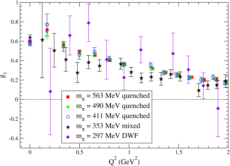
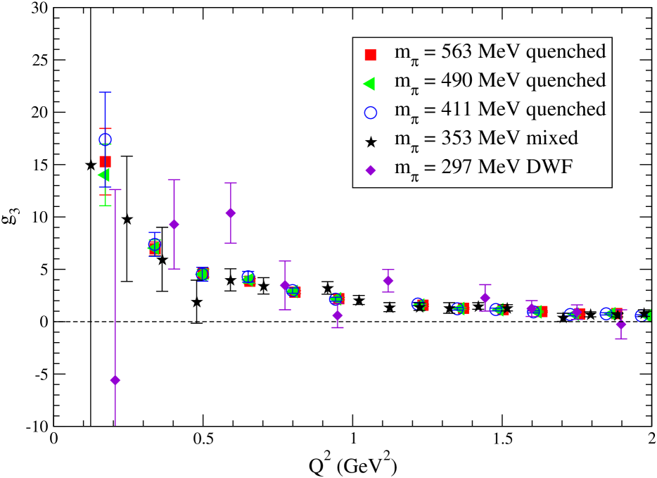
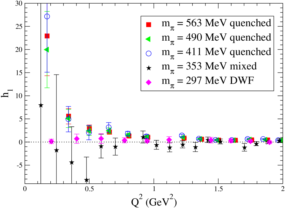
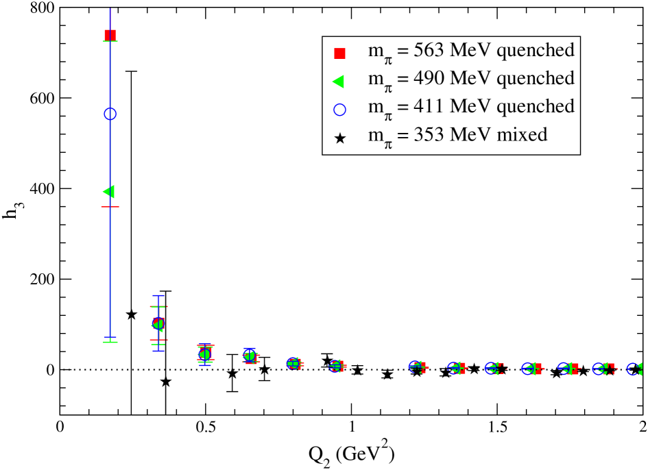
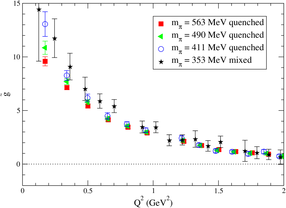
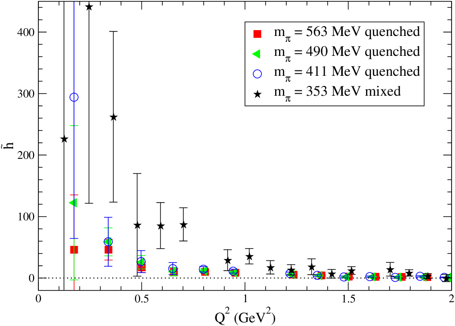
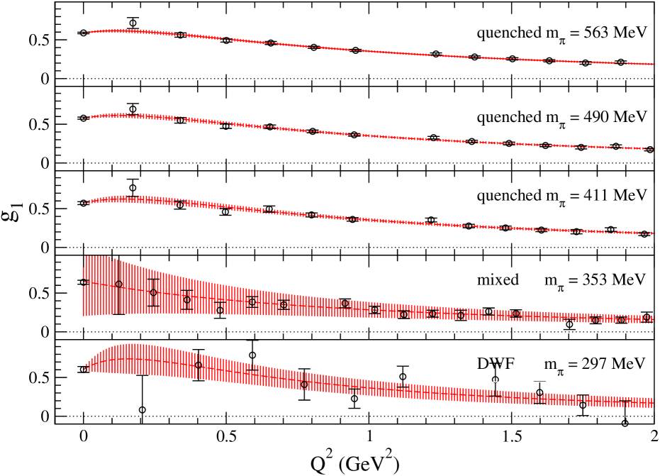
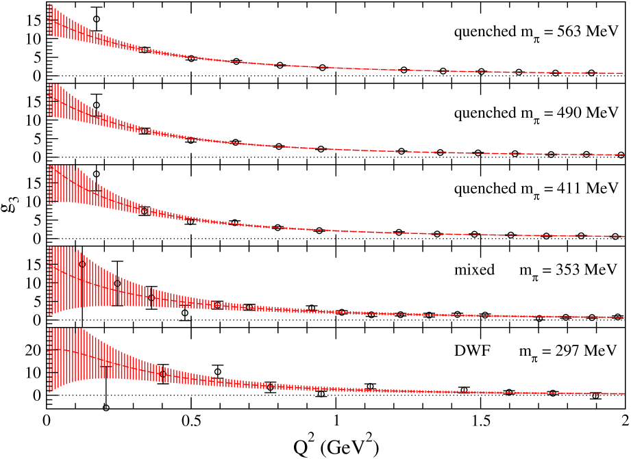
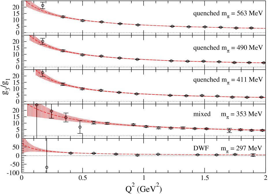
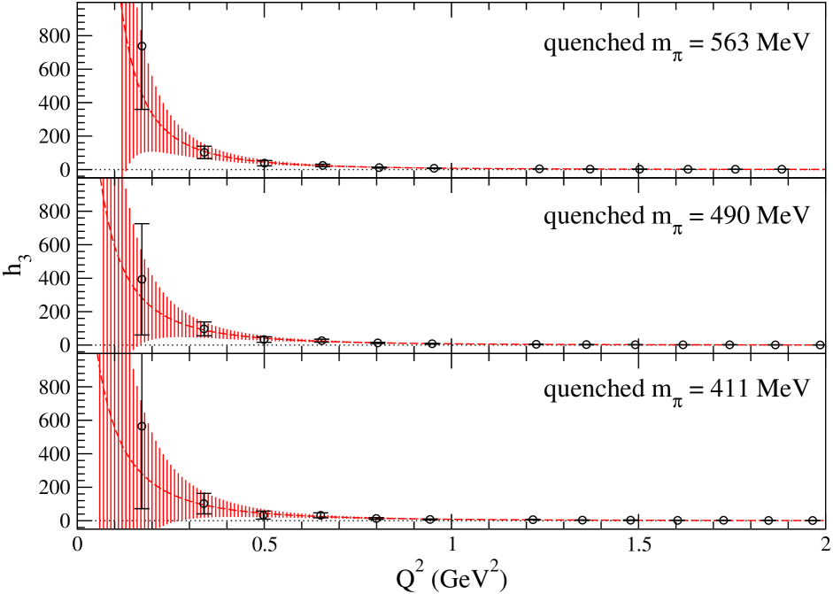
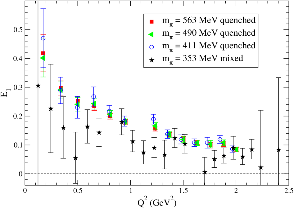
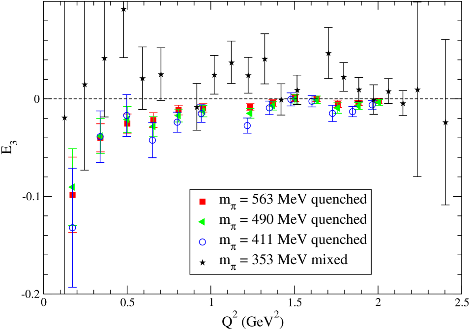
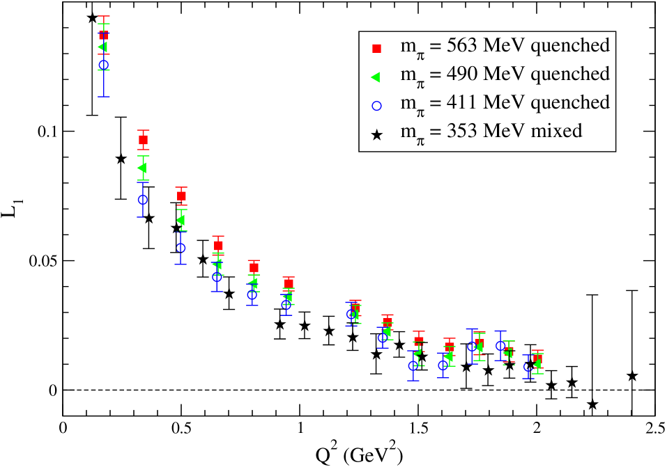
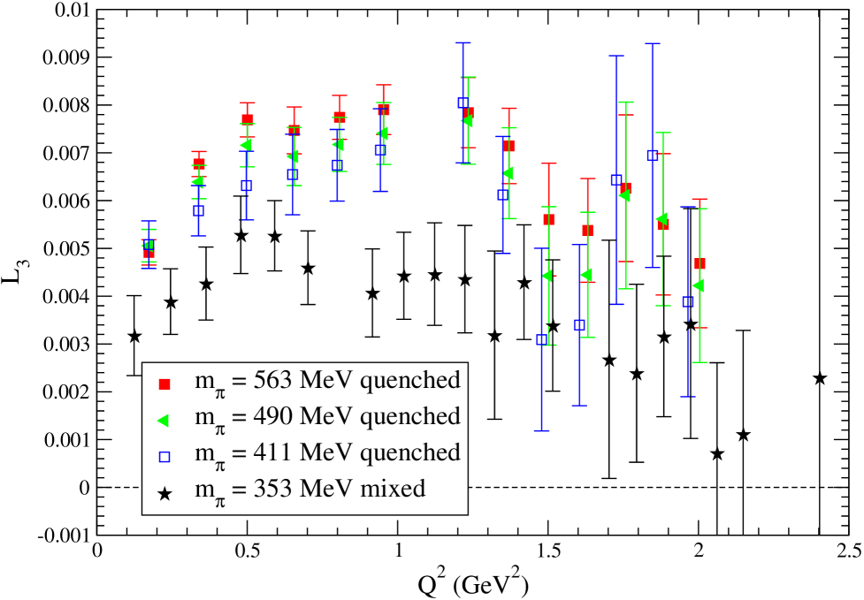
In Figs. 1, 2, 3 and 4 we show the results for the four axial form factors, , , and , respectively. All the results on these form factors are provided in Appendix C. The form factor is the dominant axial-vector form factor and the only one that can be extracted directly from the matrix element at , determining the axial charge of the . Based on PCAC and pion pole dominance we expect to be a smooth function of , whereas and to have a pion-pole and a double pion-pole behavior. Given that and are multiplied by , whereas is multiplied by it is increasingly more difficult to resolve these form factors via the simultaneous overconstrained analysis of the measured matrix element of the axial-vector current, especially at small – a fact that is clearly reflected on the statistical error of the form factors shown in the figures. The results from the quenched ensemble, although based on the analysis of 200 configurations, have the lowest statistical noise and this is the primary reason for using them in this first calculation of the form factors. The statistical noise is more severe for the DWF ensemble at MeV for which results on are too noisy to be useful and are omitted from plots. We do, however, include these numbers in the tables in the Appendix C for completeness.
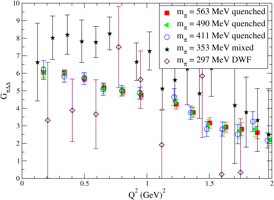
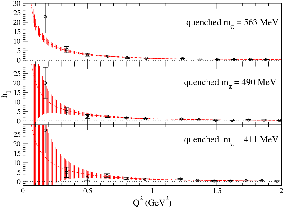
Figs. 5 and 6 show the pseudoscalar form factors and , respectively, as defined in Eq. (10), where the pion pole is explicitly written. The numerical values of these form factors are provided in Appendix C. As confirmed by the numerical results, is the dominant pseudoscalar form factor showing a pion-pole dependence, whereas the subdominant form factor shows a stronger -dependence consistent with a double pion-pole. In section II we already defined the physically relevant pion- coupling factoring out the pion-pole and fixing coefficients via PCAC through Eq. 14. has a finite value at the origin, as can be seen in Fig. 7 where numerical results are depicted. This value in fact defines the traditional strong coupling of the pion to the state via
| (45) |
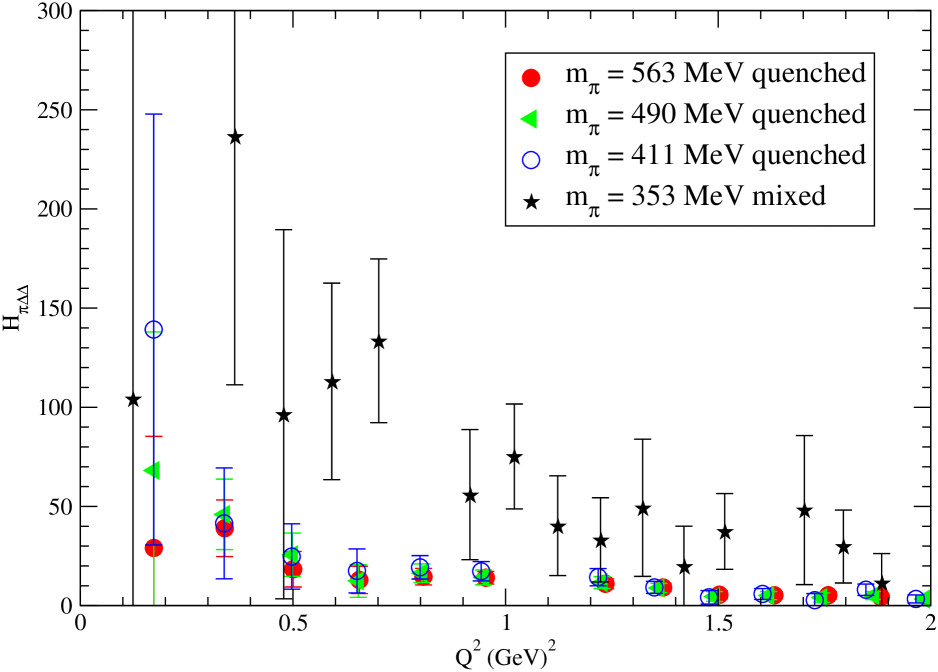
The secondary momentum-dependent coupling, , is plotted in Fig. 8. The numerical results are consisted with a pion-pole divergence at small as expected from the analysis given in the previous section. The statistical error on this coupling is larger in particular at small since in the combined analysis the pseudoscalar matrix element is multiplied by a factor of .
| or | |||
| Quenched Wilson fermions | |||
| 0.1554 | 0.0403(4) | 0.0611(14) | 0.808(7) |
| 0.1558 | 0.0307(4) | 0.0587(16) | 0.808(7) |
| 0.1562 | 0.0213(4) | 0.0563(17) | 0.808(7) |
| Hybrid or mixed action | |||
| 0.02 | 0.0324(4) | 0.0648(8) | 1.0994(4) |
| 0.01 | 0.0159(2) | 0.0636(6) | 1.0847(6) |
| DWF | |||
| 0.004 | 0.004665(3) | 0.06575(12) | 0.74521(2) |
Notice that the extraction of and from Eqs. (14) and (15) requires knowledge of the light quark mass and the pion decay constant, , on each of the ensembles. Calculation of requires the two-point functions of the axial-vector current with local-smeared (LS) and smeared-smeared (SS) quark sources,
| (46) |
(and similarly for ), where denotes the local operator and the smeared operator. The pion decay constant is obtained from the pion-to-vacuum matrix element
| (47) |
extracted from the ratio of the two-point functions and and
| (48) |
in the large Euclidean time limit.
The renormalized quark mass is determined from AWI, via two-point functions of the pseudoscalar density with either local () or smeared () quark fields,
| (49) |
(and similarly for ). The effective quark mass is defined by
| (50) |
and its plateau value yields . Note that will be needed only if ones wants alone. Since enters also Eq. (13), it cancels –as does since it comes with – and therefore and are extracted directly from ratios of lattice three- and two-point functions without prior knowledge of either or . We also note that the quark mass computed through (50) includes the effects of residual chiral symmetry breaking from the finite extent of the fifth dimension. These effects are of the order of for the DWF ensemble and for the hybrid ensemble (also referred to as mixed scheme). Chiral symmetry breaking affects the PCAC relations and therefore the value of both strong couplings and through Eq. (13).
IV.2 Testing Pion-Pole Dominance in the Axial and Pseudoscalar Matrix Element
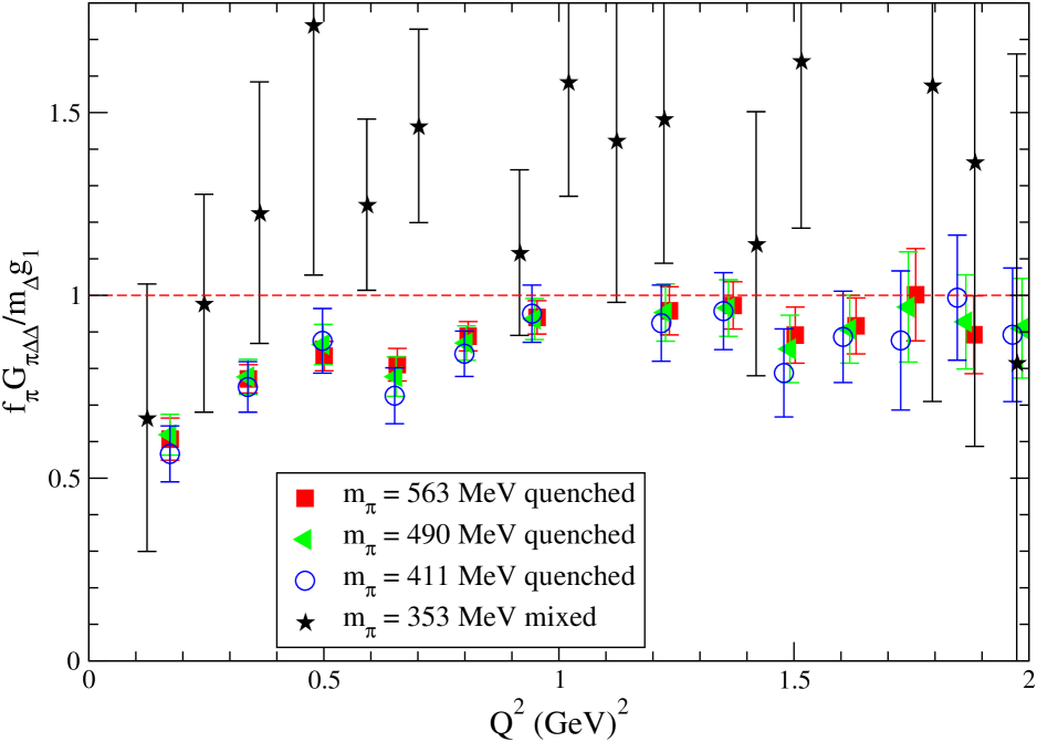
In this section we examine in detail the pion-pole dependence expected for the form factors by performing fits to the results obtained. First, we test the validity of the Goldberger-Treiman relations of Eqs. (23, 24) by evaluating the ratios
| (51) |
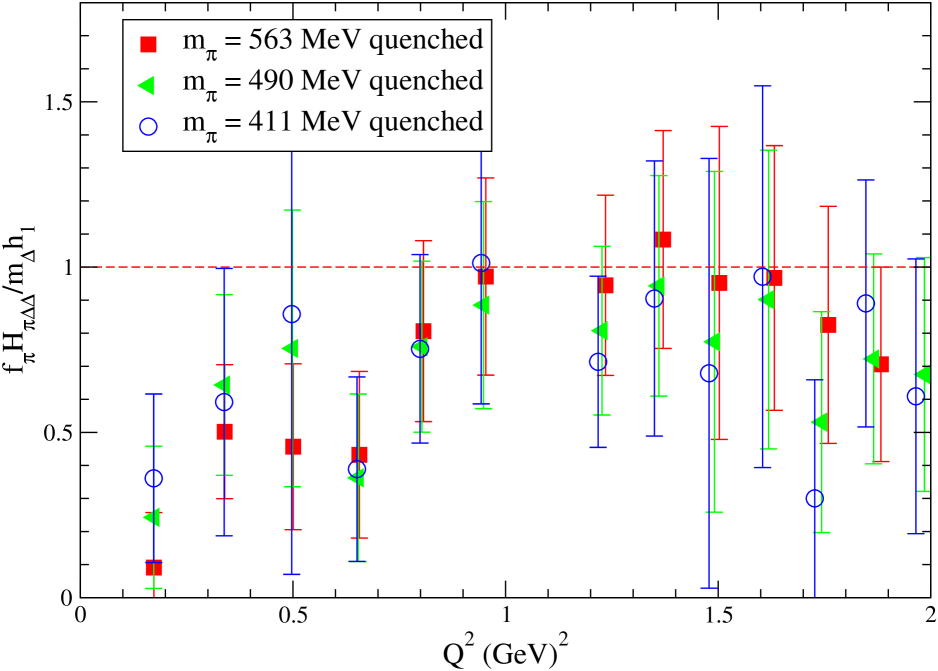
and
| (52) |
These relations are expected to hold at low . We show the results in Figs. 9 and 10. The first ratio, given in Eq. (51), carries moderate statistical error. It is consistent with unity for GeV2 for the quenched ensembles while it is underestimated at smaller values. This discrepancy at smaller can be attributed to chiral effects on , which is expected to be more seriously affected by pion cloud effects than . The results using the hybrid dynamical ensemble, on the other hand, are consistently higher than unity for GeV2. The large statistical errors carried by these data make it difficult to draw definite conclusions. The behavior of this ratio is very similar to the behavior shown by the corresponding ratio for the nucleon GT relation as well as the nucleon-to- axial transition Alexandrou et al. (2007).
The second GT-type relation, given in Eq. (52), is statistically consistent with unity for the quenched results and GeV2. The results from the dynamical ensembles are plagued by too large statistical noise to be able to meaningfully display them on the plot. We therefore have omitted these data from Fig. 10. A very similar and consistent behavior with the first ratio is observed for the quenched data. We remind the reader that it is the first Goldberger-Treiman relation that is more significant for phenomenology, as it is this relation that connects the axial charge (from at ) to the coupling.
To further probe the pion pole assumptions entering into our derivation of the GT relations we perform a set of fits to our form factor data. We have no a priori theoretical expectation for the functional form of , although typically a dipole form seems to accommodate well the nucleon axial form factor as well as the leading axial transition form factor . We note however that there seems to be a small dip in the at for the quenched ensembles. To accommodate this we fit the data to:
| (53) |
The resulting fits are shown in Fig. 11. The values for the fitted parameters are given in Table 3. We note that the mass parameter determining the slope as is around 1 GeV, a scale typical for axial dipole masses controlling the dependence of nucleon and the dominant axial form factor.
We consider the form
| (54) |
for based on the pion pole dominance prediction given in Eq.(25). The parameters , , and are fixed to the values arising from the fit of the data using the Ansatz given in Eq. (53). The fits are shown in Fig. 12. The fitted parameters are given in Table 4. Note that the value of is considerably smaller compared to , as in fact is expected since this is detected from the presence of the pion-pole. This is especially verified by the quenched data where is close to the actual pion mass of the ensemble.
Pion pole dominance fixes completely the ratio
| (55) |
We form the ratio from our data and fit separately to a monopole form:
| (56) |
This fit is displayed in Fig. 13. Using a ratio eliminates any need to know the theoretical form for alone. The fitted parameters and are given in Table 5. The verification of the predicted form given in Eq. (55) is very good, with the pole mass consistent with the pion mass and the constant reasonably close to .
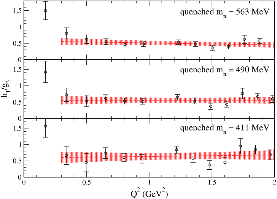
The form factor is similar to having a pion-pole dependence. We display the ratio in Fig. 14 for the quenched QCD ensembles. This ratio is notably constant over the whole range above 0.4 GeV2, with the constant . Based on this observation, we use the Ansatz given in Eq. (54) also for . The fit is shown in Fig. 15 and the fitted parameters are given in Table 6. Again, is considerably smaller compared to , in accordance to the presence of a light (pion) mode.
From Eq. (26), the ratio is completely fixed:
| (57) |
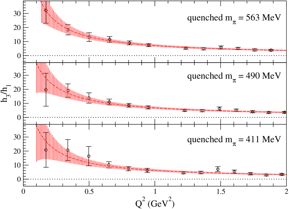
We plot this ratio in Fig. 16. Fitting the data to the monopole form of Eq. (56), we get parameters and within the range of the expected value (Eq. 57) – see Table 7 indicating that the subdominant form factor diverges with a double pion-pole- dependence.
In Fig. 17 we present the fit of to the Ansatz
| (58) |
with , , and fixed to the values extracted from the fit of . The fitted parameters and are given in Table 8, in accordance to the fit (Table 7).
In the pseudoscalar sector, one expects a monopole dependence also for the ratio . Fitting the data to the monopole form of Eq. (56), we get the parameters provided in Table 9. Indeed, an agreement of the pole mass to the pion mass within the allowed by statistical noise regime is seen.
The overall conclusion from the fits in this section is that all form factors satisfy qualitatively the pion-pole dependence predicted by PCAC. This is most clearly exemplified in the case of quenched QCD where the level of statistical noise allows such detailed analysis. In all cases the data fit these forms to good confidence levels, i.e., . Enhanced statistical noise for the dynamical ensembles limits the verification to the dominant form factors only, as the subdominant ones are beyond reach, but this still is a useful result as it shows the consistency between quenched and dynamical results. This corroborates other baryon studies that show small effects due to dynamical quark for pion masses larger than about 300 MeV.
| (GeV) | (GeV) | |||
|---|---|---|---|---|
| quenched Wilson fermions | ||||
| 0.563 | 0.53(18) | 2.15(31) | 0.98(5) | 0.82 |
| 0.490 | 0.47(18) | 2.08(33) | 0.99(6) | 1.07 |
| 0.411 | 0.40(19) | 1.98(38) | 0.94(8) | 1.48 |
| mixed action | ||||
| 0.353 | 3.0(22.0) | 2.4(1.9) | 1.3(1.2) | 0.44 |
| domain wall fermions | ||||
| 0.297 | 0.19(24) | 1.5(9) | 0.82(18) | 1.1 |
| (GeV) | (GeV) | ||
|---|---|---|---|
| quenched Wilson fermions | |||
| 0.563 | 7.77(88) | 0.54(11) | 0.61 |
| 0.490 | 7.45(89) | 0.50(11) | 0.55 |
| 0.411 | 7.1(1.0) | 0.44(15) | 0.65 |
| mixed action | |||
| 0.353 | 10.7(4.6) | 0.67(43) | 0.49 |
| domain wall fermions | |||
| 0.297 | 10.0(5.3) | 0.56(37) | 1.26 |
| (GeV) | (GeV) | (GeV2) | ||
|---|---|---|---|---|
| quenched Wilson fermions | ||||
| 0.563 | 0.523(64) | 7.60(52) | 8.64(18) | 0.67 |
| 0.490 | 0.477(63) | 7.25(49) | 8.12(18) | 0.54 |
| 0.411 | 0.396(75) | 6.76(48) | 7.64(21) | 0.60 |
| mixed action | ||||
| 0.353 | 0.61(18) | 10.4(1.6) | 9.40(33) | 0.34 |
| domain wall fermions | ||||
| 0.297 | 0.34(17) | 8.6(1.3) | 5.82(20) | 0.66 |
| (GeV) | (GeV) | ||
|---|---|---|---|
| quenched Wilson fermions | |||
| 0.563 | 3.04(48) | 1.32 | |
| 0.490 | 3.32(84) | 0.03(81) | 1.37 |
| 0.411 | 3.8(1.8) | 0.1(1.4) | 1.52 |
| (GeV) | (GeV) | (GeV4) | ||
|---|---|---|---|---|
| quenched Wilson fermions | ||||
| 0.563 | 0.26(17) | 7.6(1.1) | 8.64(18) | 0.21 |
| 0.490 | 0.31(19) | 7.4(1.1) | 8.12(18) | 0.38 |
| 0.411 | 0.28(25) | 6.7(1.1) | 7.64(21) | 0.58 |
| (GeV) | (GeV) | ||
|---|---|---|---|
| quenched Wilson fermions | |||
| 0.563 | 22(6) | 0.03(58) | 0.46 |
| 0.490 | 26(10) | 0.25(28) | 0.35 |
| 0.411 | 28(15) | 0.28(43) | 0.33 |
| (GeV) | (GeV) | ||
|---|---|---|---|
| quenched Wilson fermions | |||
| 0.563 | 0.73(39) | 4.2(1.6) | 0.23 |
| 0.490 | 0.42(43) | 3.3(1.2) | 0.22 |
| 0.411 | 0.45(70) | 3.9(2.0) | 0.32 |
V Phenomenological Couplings of the and Combined Chiral Fit
Crucial parameters in heavy baryon chiral effective theories (HBPT) with explicit degrees of freedom are the axial couplings of the nucleon, , the axial transition coupling, , and the axial charge of the , . Assuming PCAC, these can be related via GT relations to the effective , and strong couplings:
| (59) |
We note that alternative notation and normalization factors exist in the literature in the definition of the effective strong couplings for and . In addition, note that in such schemes Eqs. (59) are actually defining relations for the strong couplings. is very well known experimentally and a variety of lattice and theoretical calculations offer precise estimates. is much less-well determined, via the parity violating N-to- amplitude which connects it to the dominant axial transition form factor . remains undetermined from experiment and is typically treated –as is also the case for – as a fit parameter to be determined from fits to experimental or lattice data.
There have been several sum-rules calculations of the effective coupling Belyaev et al. (1985); Zhu (2001); Erkol . In Ref. Jido et al. (2000) symmetry arguments in a quartet scheme where , , and form a chiral multiplet, lead to the conclusion that couplings (with like-charged s) are forbidden at tree-level. Quark-model arguments Brown and Weise (1975) suggest that the .
| (GeV) | |
|---|---|
| Quenched | |
| 0.563(4) | 0.589(10) |
| 0.490(4) | 0.578(13) |
| 0.411(4) | 0.571(18) |
| Mixed action | |
| 0.498(3) | 0.573(23) |
| 0.353(2) | 0.640(26) |
| DWF | |
| 0.297(5) | 0.604(38) |
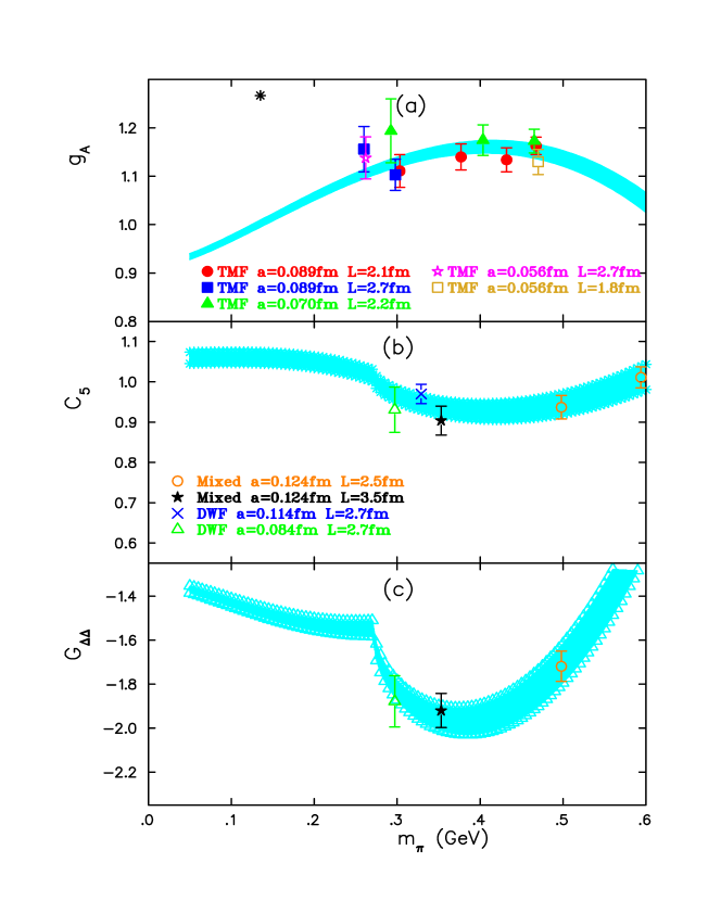
Lattice calculations for the nucleon axial charge are available on a variety of ensembles and pion masses Alexandrou et al. (2011c). In addition, results on the axial transition from factor Alexandrou et al. (2011a) have been obtained on most of the ensembles used also in this work. We are therefore in position to perform a combined chiral fit using small scale expansion (SSE) within (HBPT) Hemmert et al. (2003); Procura (2008); Jiang and Tiburzi (2008a). for , and the axial charge as functions of the pion mass .
The one-loop SSE expression for has been worked by Procura Procura (2008). The expression for as a function of is:
| (60) |
where the loop integral contribution is:
| (61) | |||||
Here , MeV, are unknown parameters and is a cutoff scale set to GeV.
We use the SSE expression for the nucleon axial charge is presented in Ref. Procura et al. (2007)
| (62) | |||||
with
| (63) |
in the above expressions denotes the chiral limit value of the axial charge, i.e. corresponds to in (61).
Finally, from Jiang and Tiburzi Jiang and Tiburzi (2008a) we obtain the chiral expansion for the axial charge of the :
| (64) | |||||
The field renormalization is
| (65) |
and the loop integrals from (Jiang and Tiburzi (2008b)) evaluated at the scale GeV:
| (66) | |||||
From the available lattice data on , and we perform a simultaneous 7-parameter fit to expressions (60),(62) and (64) fitting the unknown constants , , , as well as the common chiral couplings , and . We note that is independent of ; at a fixed value of it can be fitted as a constant.
The lattice nucleon axial charge values are taken from twisted mass simulations Alexandrou et al. (2011c). Lattice values for the real part of the axial couplings are taken from Alexandrou et al. (2011a) via a dipole extrapolation. The values of the real part of the axial charge of the , are related to the dominant axial form factor at zero momentum transfer via . For an additional lattice point to assist the fit we computed the zero-momentum values (only) on the mixed-action ensemble with MeV. Values are provided in Table 10.
In Figure 18 the combined fit is presented. The available lattice data for all three observables vary mildly in the pion mass regime considered. remains underestimated with respect to the experimental value and the inclusion of and into the SSE fit does not improve this systematically observed behavior. Strong chiral effects are expected at lighter pion mass values, especially below the decay threshold, as is evident from the 1-loop trend of and .
VI Conclusions
A detailed study of the axial structure of the has been presented, complementing recent and ongoing studies of the axial structure of the nucleon as well as the axial to transition. The matrix element of the state with the axial current has been parameterized via four Lorentz invariant form factors, and , and with two, denoted and , the pseudoscalar matrix element, generalizing the familiar nucleon axial structure. We detailed the lattice techniques required for the extraction of all six form factors for a complete dependent evaluation via specially designed three-point functions. In fact, the calculation is optimized such that only two sequential propagators are needed for the numerical evaluation of the optimal correlators. PCAC constrains strongly the nucleon matrix elements of the axial-vector and pseudoscalar currents as is manifestly evident by the phenomenological validity of the Goldberger-Treiman relation. Lattice QCD provides a check of this relation, which is a result of chiral symmetry breaking present in the QCD Lagrangian, confirming that the -dependence of the axial and pseudoscalar form factors is in agreement with the PCAC predictions. Furthermore, the recent studies of the axial to transition have shown that PCAC constrains strongly also the transition from factors and measurements of the dominant form factor and provided a check of the non-diagonal GT relation. This work, examines extensions of similar relations for the . The main result of the current work is that PCAC plays a major role also in the relation between the matrix elements of the axial-vector and pseudoscalar currents, connecting the strength of the vertex to the axial charge, . Actually, two independent pseudoscalar form factors, and are present and pion-pole dominance establishes relations among all six form factors. These predictions are qualitatively verified using results obtained in the quenched QCD study, which carries the smallest statistical noise. Results from two dynamical ensembles are consistent with these findings, albeit within large statistical errors. Having obtained an evaluation of and from previous studies and using the results of this work for on similar lattice ensembles, we performed a simultaneous chiral fit for all three utilizing one-loop chiral effective theory predictions in the SSE scheme which include a dynamical field. The seven-parameter fit does not drive the prediction near the experimentally known value, and this is not surprising as it has become recently clear that the correct value of is not reproduced even with pion masses very close to the physical one. A careful isolation of excited state effects Dinter et al. (2011); Alexandrou et al. (2011d) at pion mass of about 400 MeV failed to reveal excited state contamination in the lattice extraction of . Resolving such discrepancies is important for sharpening the predictive power of lattice QCD, which can yield phenomenologically important quantities not accessible experimentally. Fully chiral 2+1 domain wall flavour simulations are available now below the 300 MeV pion mass utilized in this work, and this leaves open the perspective for further investigations in the future which will elaborate on the relations studied in this work and on the values of the major couplings that dominate the low energy hadron interactions. However, as shown here, the gauge noise is large and noise-reduction techniques will be needed in order to extract useful results using ensembles with close to physical pion masses.
ACKNOWLEDGEMENTS
We are grateful to Brian Tiburzi and K. S. Choi for helpful discussions. EBG was supported by Cyprus Research Promotion Foundation grant and JWN in part by funds provided by the U.S. Department of Energy (DOE) under cooperative research agreement DE-FG02-94ER40818. Computer resources were provided by the National Energy Research Scientific Computing Center supported by the Office of Science of the DOE under Contract No. DE-AC02-05CH11231 and by the Jülich Supercomputing Center, awarded under the DEISA Extreme Computing Initiative, co-funded through the EU FP6 project RI-031513 and the FP7 project RI-222919. This research was in part supported by the Research Executive Agency of the European Union under Grant Agreement number PITN-GA-2009-238353 (ITN STRONGnet) and the Cyprus Research Promotion Foundation under contracts KY-A/0310/02 and NEA YOOMH/TPATH/0308/31 (infrastructure project Cy-Tera co-funded by the European Regional Development Fund and the Republic of Cyprus through the Research Promotion Foundation).
Appendix A Multipole Form Factors
The axial vector transition between states can be parameterized via a multipole expansion. This is most naturally performed on the Breit frame, where . Let us denote the matrix element as
| (67) |
Generically four different transitions will occur parameterized via
with , the longitudinal and electric multipole amplitudes of rank . The polarization vector has components , , .
We can relate the form factors , , and to the multipole form factors , , and , which have physical relevance in the multipole expansion.
| (69) |
from which the reverse relations can be verified:
| (70) | |||||
| (71) | |||||
| (72) | |||||
| (73) |
Utilizing the above relations, we present results on the four multipole axial form-factors, , , and , in Figures 19, 20, 21 and 22, respectively.
In the low momentum transfer limit, and from relations (71, 73) we deduce that . On the other hand, and remain finite, as from relation (70) and from (72) . Thus at the low momentum transfer limit we expect that .
We test these predictions explicitly in Figure 23 where the ratio is plotted. We observe a behavior consistent with a constant in the low energy regime although the numeric value of the constant is largely overestimated by the quenched lattice data. In addition, this constancy is in accordance to the pion-pole dependence of both and which is evident from the quenched lattice data plotted in Figs. (19) and (21). Despite the large statistical uncertainties, and are consistent with small values at small momentum transfers.
Appendix B Trace algebra for 3-point correlators
B.1 Axial current correlator
We define Type I as
| (74) |
After evaluating the Dirac traces we find two distinct cases, and . The kinematical frame is set to and . We note by .
For we find
| (75) | |||||
using
| (76) |
For we find
| (77) | |||||
We define Type II as:
| (78) |
| (79) |
For we find
| (80) | |||||
For we find
| (81) | |||||
B.2 Pseudoscalar density correlator
In a similar way we evaluate the trace algebra for the pseudoscalar vertices. The index summation types are defined in the same way as in the axial case. Pseudoscalar Type I is
| (82) |
After the trace evaluation we find:
| (83) | |||||
Pseudoscalar Type II is
| (84) |
giving us
| (85) |
after we evaluate the trace.
Appendix C Form Factor results
| Axial | Pseudoscalar | ||||||
|---|---|---|---|---|---|---|---|
| (GeV2) | |||||||
| 0.000000 | 0.5887(98) | — | — | — | — | — | |
| 0.1730731 | 0.717(70) | 15.3(3.2) | 22.9(8.6) | 740(380) | 9.58(43) | 46(89) | |
| 0.3396915 | 0.562(27) | 6.96(65) | 5.6(1.7) | 103(37) | 7.14(19) | 46(17) | |
| 0.5005274 | 0.491(20) | 4.63(38) | 2.89(79) | 38(16) | 5.42(18) | 17.4(8.5) | |
| 0.6561444 | 0.459(19) | 3.86(25) | 2.15(48) | 24.7(7.4) | 4.13(17) | 10.3(5.5) | |
| 0.8070197 | 0.403(14) | 2.81(15) | 1.30(26) | 11.7(3.1) | 3.44(14) | 10.1(2.9) | |
| 0.9535618 | 0.364(14) | 2.20(11) | 1.04(19) | 7.7(2.1) | 2.91(13) | 8.6(1.9) | |
| 1.235014 | 0.318(14) | 1.57(10) | 0.84(14) | 4.4(1.1) | 2.12(14) | 5.5(1.3) | |
| MeV | 1.370502 | 0.279(14) | 1.272(81) | 0.61(11) | 2.91(87) | 1.73(12) | 4.21(92) |
| 1.502826 | 0.255(14) | 1.151(89) | 0.41(11) | 2.38(79) | 1.35(13) | 2.34(90) | |
| 1.632198 | 0.230(13) | 0.959(68) | 0.388(84) | 1.97(54) | 1.17(11) | 2.08(69) | |
| 1.758807 | 0.201(17) | 0.730(86) | 0.45(11) | 1.84(64) | 1.05(14) | 1.95(72) | |
| 1.882824 | 0.211(16) | 0.769(76) | 0.439(69) | 1.69(41) | 0.92(13) | 1.52(57) | |
| 2.004400 | 0.175(14) | 0.604(65) | 0.327(58) | 1.24(31) | 0.73(10) | 1.18(43) | |
| 2.240774 | 0.124(22) | 0.43(11) | 3.249(98) | 4.66(48) | 0.40(16) | 0.48(60) | |
| Axial | Pseudoscalar | ||||||
|---|---|---|---|---|---|---|---|
| (GeV2) | |||||||
| 0.000000 | 0.578(13) | — | — | — | — | — | |
| 0.1728690 | 0.695(72) | 14.0(2.9) | 20.0(8.3) | 390(330) | 10.85(62) | 120(130) | |
| 0.3389351 | 0.550(36) | 7.03(78) | 5.1(2.0) | 97(41) | 7.69(27) | 59(23) | |
| 0.4989433 | 0.474(28) | 4.52(45) | 2.4(1.1) | 33(17) | 5.78(23) | 26(11) | |
| 0.6535119 | 0.467(23) | 3.99(31) | 2.45(60) | 26.8(9.0) | 4.23(22) | 10.3(6.8) | |
| 0.8031605 | 0.408(17) | 2.88(18) | 1.53(33) | 13.1(3.6) | 3.54(17) | 11.6(3.3) | |
| 0.9483310 | 0.363(16) | 2.18(14) | 1.14(25) | 8.1(2.4) | 2.98(16) | 8.9(2.3) | |
| 1.226705 | 0.326(17) | 1.58(12) | 1.02(18) | 5.1(1.4) | 2.21(17) | 5.9(1.5) | |
| MeV | 1.360524 | 0.278(16) | 1.253(95) | 0.67(14) | 3.2(1.0) | 1.75(14) | 4.1(1.1) |
| 1.491113 | 0.252(17) | 1.14(10) | 0.42(13) | 2.59(93) | 1.30(14) | 2.0(1.1) | |
| 1.618694 | 0.226(15) | 0.935(78) | 0.40(11) | 2.02(63) | 1.15(13) | 2.01(82) | |
| 1.743467 | 0.202(20) | 0.71(10) | 0.54(14) | 2.17(77) | 1.02(16) | 1.50(89) | |
| 1.865609 | 0.216(19) | 0.751(87) | 0.501(87) | 1.74(48) | 0.99(15) | 1.79(70) | |
| 1.985279 | 0.173(16) | 0.580(71) | 0.348(73) | 1.25(36) | 0.73(12) | 1.10(50) | |
| 2.217769 | 0.110(24) | 0.41(12) | -0.09(13) | -0.02(58) | 0.31(18) | 0.21(72) | |
| Axial | Pseudoscalar | ||||||
|---|---|---|---|---|---|---|---|
| (GeV2) | |||||||
| 0.000000 | 0.571(18) | — | — | — | — | — | |
| 0.1726468 | 0.77(11) | 17.4(4.5) | 27(12) | 560(490) | 13.1(1.1) | 290(230) | |
| 0.3381149 | 0.546(52) | 7.4(1.1) | 4.9(2.7) | 102(61) | 8.27(45) | 59(40) | |
| 0.4972318 | 0.458(44) | 4.53(66) | 2.0(1.6) | 33(24) | 6.17(36) | 27(18) | |
| 0.6506769 | 0.495(41) | 4.28(51) | 3.2(1.0) | 32(15) | 4.48(31) | 15.4(9.8) | |
| 0.7990168 | 0.419(26) | 2.96(25) | 1.81(49) | 13.4(5.2) | 3.73(23) | 14.4(4.4) | |
| 0.9427295 | 0.361(23) | 2.14(19) | 1.21(37) | 7.5(3.4) | 3.16(22) | 11.2(3.2) | |
| 1.217848 | 0.354(25) | 1.68(16) | 1.42(26) | 6.4(2.0) | 2.41(25) | 7.5(2.3) | |
| MeV | 1.349909 | 0.276(22) | 1.23(12) | 0.72(21) | 3.4(1.4) | 1.78(18) | 4.4(1.4) |
| 1.478675 | 0.251(24) | 1.16(13) | 0.44(19) | 3.1(1.3) | 1.23(18) | 1.8(1.5) | |
| 1.604379 | 0.224(20) | 0.93(10) | 0.43(16) | 2.26(87) | 1.15(16) | 2.4(1.1) | |
| 1.727230 | 0.203(28) | 0.68(13) | 0.65(21) | 2.5(1.1) | 0.96(21) | 1.0(1.3) | |
| 1.847415 | 0.230(24) | 0.75(11) | 0.63(13) | 1.87(64) | 1.16(20) | 2.9(1.0) | |
| 1.965099 | 0.171(18) | 0.565(85) | 0.39(10) | 1.32(47) | 0.73(15) | 1.13(68) | |
| 2.193551 | 9.100(30) | 0.37(14) | -0.18(19) | 8.70(83) | 0.16(21) | -0.2(1.1) | |
| Axial | Pseudoscalar | ||||||
|---|---|---|---|---|---|---|---|
| (GeV2) | |||||||
| 0.000000 | 0.640(26) | — | — | — | — | — | |
| 0.1240682 | 0.62(39) | 15(26) | 8(74) | -100(4500) | 14.4(4.8) | 230(1800) | |
| 0.2450231 | 0.51(17) | 9.8(6.0) | -2(16) | 120(540) | 11.7(1.8) | 440(320) | |
| 0.3630880 | 0.41(12) | 6.0(3.1) | -4.4(7.7) | -25(200) | 9.1(1.2) | 260(140) | |
| 0.4784607 | 0.28(10) | 1.9(2.1) | -8.1(4.9) | -160(104) | 7.0(1.1) | 87(83) | |
| 0.5913172 | 0.385(69) | 4.0(1.1) | -0.9(2.5) | -7(40) | 5.88(67) | 85(37) | |
| 0.7018154 | 0.349(60) | 3.42(78) | -1.0(1.9) | 2(25) | 5.41(61) | 87(27) | |
| 0.9162911 | 0.368(57) | 3.22(60) | 1.1(1.3) | 21(15) | 3.46(56) | 29(17) | |
| 1.020513 | 0.283(47) | 2.07(43) | -0.6(1.0) | -0.3(9.3) | 3.43(51) | 35(12) | |
| 1.122869 | 0.222(50) | 1.39(43) | -1.15(98) | -9.6(8.5) | 2.22(52) | 17(11) | |
| 1.223456 | 0.234(45) | 1.43(36) | -0.50(77) | -3.2(6.3) | 2.26(48) | 13.3(8.5) | |
| MeV | 1.322363 | 0.212(66) | 1.31(51) | -1.1(1.0) | -5.6(8.1) | 2.34(77) | 18(13) |
| 1.419670 | 0.262(46) | 1.50(31) | 0.48(60) | 2.5(4.2) | 1.70(50) | 7.0(7.1) | |
| 1.515454 | 0.237(48) | 1.32(30) | 0.12(53) | 2.0(3.6) | 2.08(54) | 12.3(6.3) | |
| 1.702723 | 9.586(67) | 0.41(38) | -1.15(83) | -6.4(4.8) | 1.25(99) | 14(11) | |
| 1.794332 | 0.148(44) | 0.70(24) | -0.35(44) | -1.8(2.5) | 1.07(56) | 8.4(5.2) | |
| 1.884666 | 0.151(39) | 0.65(20) | 0.00(66) | -0.3(2.0) | 0.90(48) | 3.1(4.0) | |
| 1.973777 | 0.190(66) | 0.82(32) | 0.34(44) | 1.3(2.3) | 0.65(67) | -6.1(5.8) | |
| 2.061714 | 0.141(42) | 0.66(20) | 0.05(35) | 0.5(1.8) | 0.37(52) | 5.4(4.0) | |
| 2.148521 | 0.173(56) | 0.77(26) | 0.38(35) | 2.1(1.7) | 1.07(59) | 4.3(4.1) | |
| 2.234241 | 0.06(31) | 0.4(1.6) | -0.1(2.6) | 0.0(11.0) | -0.5(3.5) | -5(32) | |
| 2.402577 | 0.14(39) | 0.5(1.5) | 0.7(2.3) | 2.5(9.2) | 1.0(3.4) | 2(18) | |
| Axial | Pseudoscalar | ||||||
|---|---|---|---|---|---|---|---|
| (GeV2) | |||||||
| 0.0 | 0.604(38) | — | — | — | — | — | |
| 0.2060893 | 0.08(45) | -5.6(18.0) | -44(45) | -1500(2000) | 9.4(9.3) | -1100(1800) | |
| 0.4030337 | 0.66(20) | 9.3(4.3) | 11(10) | 130(240) | 6.6(3.0) | -300(280) | |
| 0.5919523 | 0.79(19) | 10.3(2.9) | 13(6) | 210(110) | 4.5(2.4) | -82(140) | |
| 0.7737530 | 0.41(20) | 3.5(2.3) | 2.2(5.2) | 8(65) | 7.2(2.2) | 125(90) | |
| 0.9491845 | 0.21(12) | 0.6(1.7) | -1.0(2.5) | -34(25) | 4.5(1.3) | 42(39) | |
| 1.118873 | 0.51(14) | 3.9(1.1) | 4.8(2.2) | 45(19) | 1.3(1.4) | -20(32) | |
| 1.443061 | 0.47(21) | 2.3(1.3) | 4.3(2.6) | 21(17) | 3.2(1.9) | 27(30) | |
| 1.598405 | 0.31(14) | 1.25(76) | 2.1(1.6) | 4.7(8.8) | 0.1(1.2) | -1(16) | |
| 1.749719 | 0.14(13) | 0.91(69) | 0.0(1.3) | 2.2(7.2) | 0.2(1.4) | -12(16) | |
| 1.897302 | -0.09(29) | -0.3(1.4) | -2.2(3.2) | -11(16) | -4.6(4.6) | -62(57) | |
| MeV | 2.041417 | -0.03(33) | 0.1(1.6) | -0.4(2.9) | 3(14) | 0.2(3.1) | 6(33) |
| 2.182297 | 0.17(23) | 0.51(91) | 0.8(1.8) | 4.6(7.7) | 2.8(2.7) | 9(18) | |
| 2.320150 | -0.06(14) | -0.41(57) | -0.7(1.1) | -3.6(4.4) | 0.4(1.4) | 2(11) | |
References
- Jansen (2008) K. Jansen (2008), eprint 0810.5634.
- Durr et al. (2008) S. Durr et al., Science 322, 1224 (2008).
- Aoki et al. (2009) S. Aoki et al. (PACS-CS), Phys. Rev. D 79, 034503 (2009), eprint 0807.1661.
- Durr et al. (2011) S. Durr, Z. Fodor, C. Hoelbling, S. Katz, S. Krieg, et al., JHEP 1108, 148 (2011), eprint 1011.2711.
- Alexandrou et al. (2009a) C. Alexandrou et al. (ETM Collaboration), Phys.Rev. D80, 114503 (2009a), eprint 0910.2419.
- Aoki et al. (2010) S. Aoki et al. (PACS-CS Collaboration), Phys.Rev. D81, 074503 (2010), eprint 0911.2561.
- Beane et al. (2012) S. Beane et al. (NPLQCD Collaboration), Phys.Rev. D85, 034505 (2012), eprint 1107.5023.
- Dudek et al. (2012) J. J. Dudek, R. G. Edwards, and C. E. Thomas, Phys.Rev. D86, 034031 (2012), eprint 1203.6041.
- Feng et al. (2010) X. Feng, K. Jansen, and D. B. Renner, Phys.Lett. B684, 268 (2010), eprint 0909.3255.
- Yamazaki et al. (2004) T. Yamazaki et al. (CP-PACS Collaboration), Phys.Rev. D70, 074513 (2004), eprint hep-lat/0402025.
- Kotulla et al. (2002) M. Kotulla, J. Ahrens, J. Annand, R. Beck, G. Caselotti, et al., Phys.Rev.Lett. 89, 272001 (2002), eprint nucl-ex/0210040.
- Lopez Castro and Mariano (2001) G. Lopez Castro and A. Mariano, Phys.Lett. B517, 339 (2001), eprint nucl-th/0006031.
- Bernard et al. (2005) V. Bernard, T. R. Hemmert, and U.-G. Meissner, Phys.Lett. B622, 141 (2005), eprint hep-lat/0503022.
- Hemmert et al. (1998) T. R. Hemmert, B. R. Holstein, and J. Kambor, J.Phys. G24, 1831 (1998), eprint hep-ph/9712496.
- Jenkins and Manohar (1991) E. E. Jenkins and A. V. Manohar, Phys.Lett. B259, 353 (1991).
- Fettes and Meissner (2001) N. Fettes and U. G. Meissner, Nucl.Phys. A679, 629 (2001), eprint hep-ph/0006299.
- Bernard (2008) V. Bernard, Prog.Part.Nucl.Phys. 60, 82 (2008), eprint 0706.0312.
- Dashen et al. (1994) R. F. Dashen, E. E. Jenkins, and A. V. Manohar, Phys.Rev. D49, 4713 (1994), eprint hep-ph/9310379.
- Brown and Weise (1975) G. Brown and W. Weise, Phys.Rept. 22, 279 (1975).
- Choi et al. (2010) K.-S. Choi, W. Plessas, and R. Wagenbrunn, Phys.Rev. D82, 014007 (2010), eprint 1005.0337.
- Alexandrou et al. (2007) C. Alexandrou, G. Koutsou, T. Leontiou, J. W. Negele, and A. Tsapalis, Phys.Rev. D76, 094511 (2007), eprint 0912.0394.
- Alexandrou et al. (2011a) C. Alexandrou, G. Koutsou, J. Negele, Y. Proestos, and A. Tsapalis, Phys.Rev. D83, 014501 (2011a), eprint 1011.3233.
- Alexandrou et al. (2009b) C. Alexandrou, T. Korzec, G. Koutsou, C. Lorce, J. W. Negele, et al., Nucl.Phys. A825, 115 (2009b), eprint 0901.3457.
- Alexandrou et al. (2012) C. Alexandrou, C. Papanicolas, and M. Vanderhaeghen (2012), eprint 1201.4511.
- Alexandrou et al. (2011b) C. Alexandrou, E. B. Gregory, T. Korzec, G. Koutsou, J. W. Negele, et al., Phys.Rev.Lett. 107, 141601 (2011b), eprint 1106.6000.
- Alexandrou et al. (2011c) C. Alexandrou et al. (ETM Collaboration), Phys.Rev. D83, 045010 (2011c), eprint 1012.0857.
- Jiang and Tiburzi (2008a) F.-J. Jiang and B. C. Tiburzi, Phys.Rev. D78, 017504 (2008a), eprint 0803.3316.
- (28) Http://www.nikhef.nl/form.
- Tsapalis (2006) A. Tsapalis, Nucl.Phys.Proc.Suppl. 153, 320 (2006).
- Bernard et al. (2001) C. W. Bernard, T. Burch, K. Orginos, D. Toussaint, T. A. DeGrand, et al., Phys.Rev. D64, 054506 (2001), eprint hep-lat/0104002.
- Aoki et al. (2011) Y. Aoki et al. (RBC Collaboration, UKQCD Collaboration), Phys.Rev. D83, 074508 (2011), eprint 1011.0892.
- Belyaev et al. (1985) V. Belyaev, B. Y. Blok, and Y. Kogan, Sov.J.Nucl.Phys. 41, 280 (1985).
- Zhu (2001) S.-L. Zhu, Phys.Rev. C63, 018201 (2001), eprint nucl-th/0009062.
- (34) G. Erkol, http://irs.ub.rug.nl/ppn/297396218.
- Jido et al. (2000) D. Jido, T. Hatsuda, and T. Kunihiro, Phys.Rev.Lett. 84, 3252 (2000), eprint hep-ph/9910375.
- Hemmert et al. (2003) T. R. Hemmert, M. Procura, and W. Weise, Phys.Rev. D68, 075009 (2003), eprint hep-lat/0303002.
- Procura (2008) M. Procura, Phys.Rev. D78, 094021 (2008), eprint 0803.4291.
- Procura et al. (2007) M. Procura, B. Musch, T. Hemmert, and W. Weise, Phys.Rev. D75, 014503 (2007), eprint hep-lat/0610105.
- Jiang and Tiburzi (2008b) F.-J. Jiang and B. C. Tiburzi, Phys.Rev. D77, 094506 (2008b), eprint 0801.2535.
- Dinter et al. (2011) S. Dinter, C. Alexandrou, M. Constantinou, V. Drach, K. Jansen, et al., Phys.Lett. B704, 89 (2011), eprint 1108.1076.
- Alexandrou et al. (2011d) C. Alexandrou, M. Constantinou, S. Dinter, V. Drach, K. Jansen, et al., PoS LATTICE2011, 150 (2011d), eprint 1112.2931.